Modification of the Bellman–Ford Algorithm for Finding the Optimal Route in Multilayer Network Structures

Abstract

One of the actual tasks of the contemporary logistics business using the “just in time” supply planning concept, is to distribute manufactured goods among the objects of the distribution network in the most efficient manner at the lowest possible cost. The article is devoted to the problem of finding the optimal path in network structures. The problem statement for multilayer data transmission networks (MDTN), which is one of the possible representations of multimodal transport networks, is considered. Thus, each MDTN layer can be represented as a separate type of transport. The problem is solved by modifying the Bellman–Ford mathematical programming algorithm. Load testing of the modified method was performed, and a comparative analysis was given, including an assessment of speed and performance, proving the effectiveness of the results of the study. Based on the results of comparative analysis, recommendations for using a modified version of the Bellman–Ford algorithm for application in practical problems in optimizing logistics networks are proposed. The results obtained can be used in practice not only in logistics networks but also in the construction of smart energy networks, as well as in other subject areas that require optimization of multilayer graph structures.

1. Introduction

Nowadays, network structures are one of the most popular types of visualization of various information in many areas of science and society. Graph visualization is widely used in the management of logistics and smart electrical networks, information security, and many other areas of modern activities.

As a network structure, we will use a goods distribution network, which is a graph representation of the subjects that are necessary for transporting products from the manufacturer to the end consumer. The aim of the work is to determine the optimal route for delivering the product from the point of production to the final consumer, which provides for minimal costs for material, labor and time resources. Modeling the operation of such a network will optimize the plan for the supply of products, taking into account the impact of external factors, which will ensure the rational work of the manufactory. Nowadays, multimodal transportation, which is a more flexible type of transporting goods than classical commodity distribution networks due to the ability to use several types of transport, has become widely used in the logistics sector. To optimize such logistics networks, it is possible to use multilayer graph models.

The main goal of supply chain management is to reduce economic costs and meet the needs of customers in the final product.

The supply chain is a set of links interconnected by information, cash and commodity flows and includes the stages of planning, procurement, production, delivery and return of goods.

2. Literature Review

A goods distribution network, as one of the varieties of network structures, is a connected structure consisting of system elements, including graph vertices and transition states between them. Such connections between vertices are referred to as edges. Thus, in [1,2,3,4] the problem of supply chain management is solved with the optimization of the parameters spent on the transportation of goods and profit maximization, respectively. In [5,6], the problem of optimizing the consumption of electricity, ensuring its uninterrupted supply and restructuring the network in case of failure of the nodes of the graph structure (switches) is solved. In this case, the nodes of the graph are network switches, and the arcs are power transmission lines.

One of the main problems solved by network structures is the APSP problem (all pairs shortest path problem)—the problem of finding the optimal route on a given space of states. Over its almost half-century history, many algorithms have been created to solve this problem, ranging from the method of exhaustive enumeration of all possible solutions to modified genetic algorithms. Thus, in [7,8,9] a logistics network of multimodal transportation is presented in the form of a graph structure. The nodes of the graph are production points, warehouses and points of consumption of products, distribution centers for loading and unloading goods and the arcs are various types of transportation. The weight of the arc means the cost of transportation and includes various factors, such as the time and cost of transportation, the seasonality of the product, its transportability, and others.

Various deterministic, heuristic methods and artificial intelligence algorithms are used to optimize network structures. One of the first methods was Dijkstra’s algorithm, according to which each vertex of the graph was associated with the minimum known distance from this vertex to the desired one, the so-called labels. Further, at each step, the method “visits” the next vertex and tries to reduce the labels. The algorithm terminates when all vertices have been visited. Currently, there are many new modifications of this algorithm, considered in [10,11].

By now, Dijkstra’s algorithm has undergone different modifications and other algorithms, based on it, have appeared. For example, the Floyd–Warshall algorithm gained wide popularity. The method belongs to dynamic programming methods for finding the minimum distances between graph vertices. The main advantage of the algorithm is that it can be successfully applied to a weighted graph with both positive and negative edge weights [12].

One of the latest algorithms developed for finding the shortest path in graph structures was Jump Point Search (JPS), described by Australian scientists D. Harbor and A. Gradshtein in [13,14]. The algorithm was obtained by modifying the A* method [15] and applied to an indefinite graph. The goal is to recursively traverse all points that can be reached by an optimal path that does not pass through the current position. The exit from the recursion is carried out after hitting the so-called “jump point successor” and the process for this node starts again.

Thus, the problem of optimization of graph structures finds more application in problems of various applied areas. For this purpose, adaptation, modification and development of previously known algorithms are carried out annually. In this article, a method for solving the APSP problem for a network model consisting of several layers is considered. The novelty of the work is the adaptation of the Bellman–Ford algorithm for finding the shortest route in a multilayer data transmission network.

3. Problem Formulation

A multilayer data transmission network (MDTN) or a network model is a collection of several layers representing a pool of undirected graphs ${G_m,m\in 1..z}_{}$, where z is the number of graphs in the model, built on a set of a vertices V_m∈{v₁,…,v_n}. 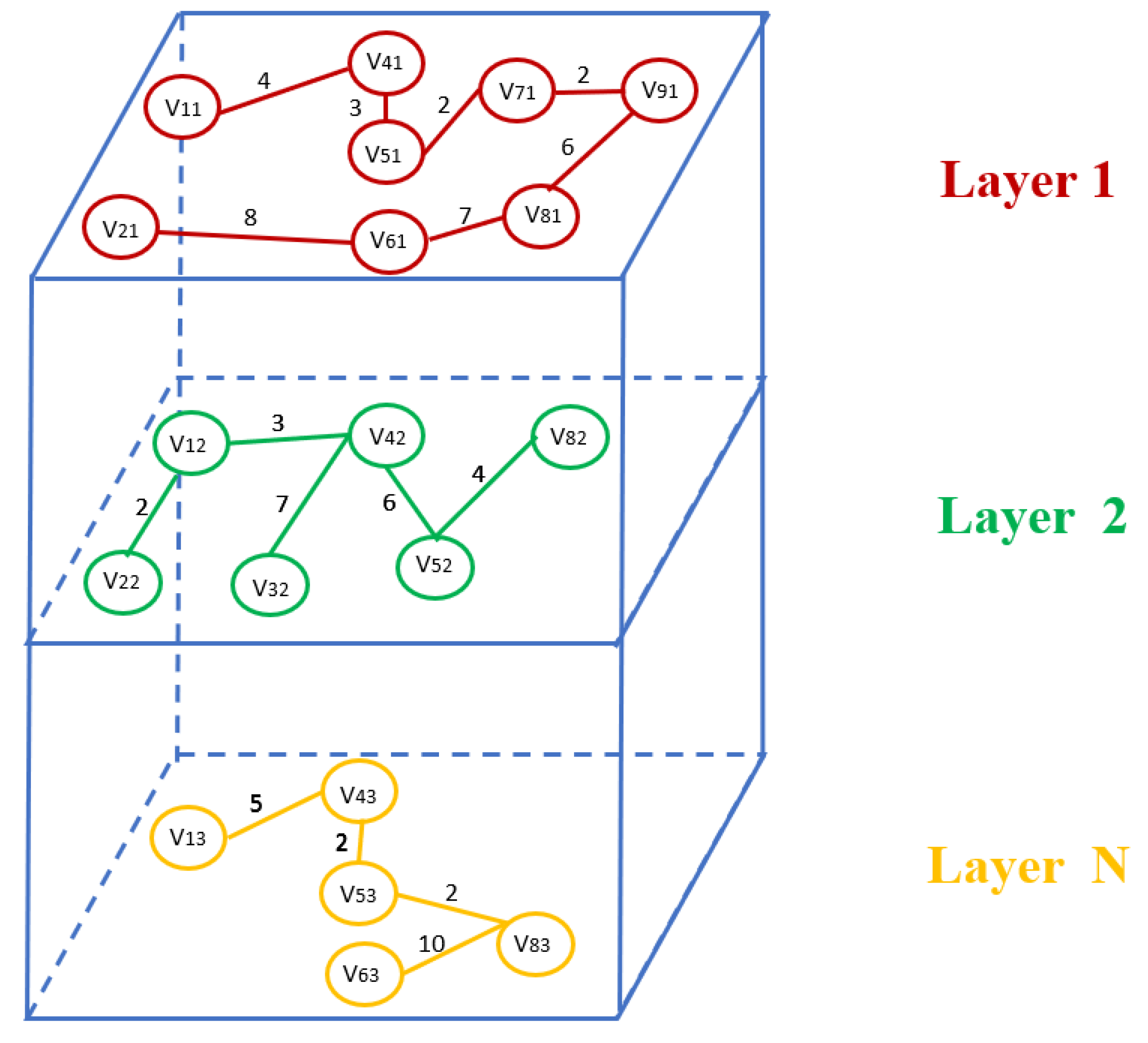Edges of graph G_m$E_{i,j}^m$ have certain weight coefficients $k_{i,j}^m$, where i,j are the serial numbers of the vertices from V_m, which are connected by the edge $E_{i,j}^m$ in the graph G_m, m∈1..z, i,j∈1..n. Units of weight coefficients may vary depending on the subject area of the task. The designations of the graph structure have a composite index, in which n is the ordinal number of the vertex and m is the number of the layer to which the given node belongs. For example, the third vertex located in the second layer will be denoted as V₃₂ [11]. Graphical visualization of the MDTN model is presented in Figure 1. The units of the parameter may vary depending on the subject area of the task.

The task is to find the shortest path for the resulting graph after the operation of combining all its layers.

The union of two graphs G₁ and G₂ is called a graph G₃, which consists of the union of all vertices and edges of the original layers (1).

$$G_1(V_1,E_1)\cup G_2(V_2,E_2)=G_3(V_3,E_3)={(V_3=V}_1\cup V_2,{E_3=E}_1\cup E_2),$$

(1)

The merged MDTN shown in Figure 1 is presented in Figure 2.

In Figure 2, the edges are highlighted in different colors: red for the first layer, green for the second, and yellow for the third layer of the considered MDTN, respectively. After merging, the MDTN needs to be preprocessed. Let us consider the problem using the example of N = 3.

A path in an undirected graph layered structure is a sequence of interconnected vertices P = {$v_{l,m},\dots ,v_{s,m}$}∈V, m∈{1,…,z}, l,s∈{1,…,n}. Such a path P is called a path from $v=v_{l,m} \mathrm{t}\mathrm{o} v^{\prime }=v_{s,m}$.

The weight coefficient of edge $e_{i,j}^m$ is $k_{i,j}^m$. The weight function (2), which maps the edges to their corresponding weights, representing the set of real numbers, is known.

$$f:E\to R.$$

(2)

Then, the shortest path from vertex v to vertex v’ is the path $P_{min}$ = {$v_{l,m},\dots ,v_{s,m}$}∈V, where $v_{l,m}=v$, $v_{s,m}=v\prime$, which satisfies the value objective function represented by Formula (3).

$$\sum _{\begin{array}{c}i=l\\ i,j∊P\end{array}}^s\sum _{m=1}^z{k}_{i,j}^m\to min.$$

(3)

If all edges in the graph have unit weight, then the problem is reduced to determining the least number of traversed edges.

Multilayer data transmission networks can be widely used in supply chain management in tasks of the logistics sphere. The supply chain management process is a simulation of the transportation of manufactured goods through intermediate warehouses to the final consumer. The most common and optimal scheme of work is the “just in time” system, which is characterized by the following features:

-

Stable production output at each time step;

-

Frequent deliveries of products in small batches;

-

Lack of supply with excess or deficiency.

For the transportation of products, it is possible to use multimodal logistics networks using various types of transport. Thus, each MDTN layer can represent different types of transport, and the nodes of the layer in this case are the reference points for transporting products with the possibility of reloading products from one type of transport to another, and the edges are the links between them.

Thus, when optimizing MDTN, the process of choosing the best route for products between given points according to the established parameters takes place.

4. Materials and Methods

4.1. MDTN Preprocessing

Finding the shortest path will be carried out using the Bellman–Ford algorithm. The modification of the algorithm consists in adding to it the preprocessing of the initial data, which will increase the efficiency of finding optimal paths in multimodal transport networks. The purpose of data preprocessing is to make sure that the graphs, which are constructed from the reachability matrix, are connected and do not have cycles and loops. A graphical representation of the designed system is shown using a data flow diagram (DFD) in Figure 3.

A graph is called connected if there is only one connected component, i.e., when any two vertices of G (x, y) are connected by at least one path. Otherwise, the graph is called disconnected [16]. An example of a connected graph is shown in Figure 2.

To determine the connectivity, the algorithm of bypassing the graph model in breadth (breadth-first search) [17] is used. In this method, connectivity is checked by viewing all possible directions from a given vertex of the graph with the transition to a higher level at each iteration. Thus, the algorithm, starting from the source vertex s, includes in the search all nodes connected by edges to the given vertex. Next, the transition process to the obtained vertices is carried out and the browsing continues until the next attempt to browse the next vertices does not find any new nodes of the graph.

Next, the check of the presence of cycles in the network structure is needed. If there are such, it is possible that there are many shortest paths from a given vertex of the cycle to another, since each iteration of the loop reduces the length of the path [18]. Brent’s algorithm was used to eliminate cycles. The algorithm is chosen due to the fact that, on average, it works about 36% faster than the Floyd algorithm and about 24% faster than the Pollard algorithm in solving a similar problem [19].

To describe the Brent algorithm, denote by M the set consisting of m elements. Additionally, define mapping f:M→M and an arbitrary element a₀ belonging to the set under consideration. Next, consider the sequence of elements a₀, a₁, …, a_n defined by equality (4).

$$a_{n+i}=f\left(a_n\right),n=\mathrm{0,1},\dots .$$

(4)

Since the considered set M is finite, the sequence (4) can be looped from some arbitrary moment. In this case, the cycle can be started from any element ${\mathit{a}}_{\mathit{\gamma }}$ so that equality (5) is satisfied.

$$a_n=a_{n+\tau }, \mathrm{f}\mathrm{o}\mathrm{r} \mathrm{a}\mathrm{l}\mathrm{l} n\ge \gamma \ge \tau \mathrm{a}\mathrm{n}\mathrm{d} \tau \ge 1,$$

(5)

where γ is the length of the approach to the cycle, τ is the length of the cycle [20].

Thus, the problem of finding cycles in a graph structure is carried out with known mappings f and start element a₀. The block diagram of the Brent method is shown in Figure 4.

The main advantages of this algorithm are that no additional steps are required to find and determine the correct cycle length τ, and the calculation function is called at each iteration step only once.

The performance speed of the method is O(g + τ), where g is the smallest index of the sequence that is the beginning of the cycle, and τ is the length of the cycle. The MDTN considered in Figure 1 after the removal of cycles in it is shown in Figure 5.

The Bellman–Ford algorithm is applied to the resulting graph to find the optimal path.

4.2. Finding the Optimal Route

The Bellman–Ford algorithm was created by American scientists as a distance vector routing (RIP) method that deals with transit sections between two network nodes through which network packets are transmitted. Later, the algorithm was further developed for the problems of finding the minimum route of weighted network structures. Let us consider step by step structure of the algorithm.

Step 1. In a given graph G with edge weights ${\mathit{k}}_{\mathit{i}\mathit{j}}$, the initial source vertex ${\mathit{v}}_{\mathit{i}}$, from which the shortest route will be searched, is determined.

Step 2. An array of distances d [0, 1, …, (q − 1)], where q is the number of vertices in the graph, is specified. After the algorithm is executed, this array will contain the solution to the problem of finding the optimal route. Initially, the array is initialized according to Formula (6).

$$\begin{array}{c}d\left(v_1\right)=0, where v_1-\mathrm{s}\mathrm{t}\mathrm{a}\mathrm{r}\mathrm{t} \mathrm{v}\mathrm{e}\mathrm{r}\mathrm{t}\mathrm{e}\mathrm{x} \mathrm{o}\mathrm{f} \mathrm{s}\mathrm{h}\mathrm{o}\mathrm{r}\mathrm{t}\mathrm{e}\mathrm{s}\mathrm{t} \mathrm{p}\mathrm{a}\mathrm{t}\mathrm{h} \mathrm{s}\mathrm{e}\mathrm{a}\mathrm{r}\mathrm{c}\mathrm{h}\\ d\left(v_i\right)=\mathrm{\infty }.\end{array}$$

(6)

Step 3. Computational core. The main operation of the algorithm is the operation of edge relaxation. Edge relaxation is the process of improving the value of the optimal route obtained at the previous iteration of the algorithm. At each iteration, the algorithm looks through all the edges of the graph and tries to relax along each edge (u, v) that has cost c. Algorithmically, the core relaxation function is described in formula 7.

$$\mathrm{i}\mathrm{f} d\left[v\right]>\left(d\left[u\right]+c\right),\mathrm{e}\mathrm{l}\mathrm{s}\mathrm{e} d\left[v\right]=\left(d\left[u\right]+c\right).$$

(7)

For unreachable vertices from the current node, the distance $d\left(v_i\right)$ remains equal to infinity. A graphical representation of the relaxation process is shown in Figure 6.

Step 4. The algorithm iteratively refines the value of the function d(v) at each step until the process of relaxation of at least one edge occurs at the iteration.

In its work, the Bellman–Ford algorithm can maximally perform (|V| − 1) iteration over the relaxation of E edges. Therefore, its performance speed is defined as O(|V||E|). This parameter can be reduced by applying graph preprocessing by removing all cycles.

Figure 7 shows the optimal route between vertices V₂V₉ for the initial MDTN.

4.3. Calculation of the Coefficient of Admissibility of Decisions

The resulting solution is optimal. The optimal route is the only path by which you can get from a given vertex to the final one with minimal losses. However, there are tasks for which it is necessary to have backup shortest routes. Such options with a certain degree of fault tend to the weight of the optimal route, therefore, it is necessary to consider the possibility of forming a pool of paths that are not optimal, but close in cost to them. Let us call such routes admissible.

The formation of admissible routes occurs after the determination of the optimal path and implies a deviation from the cost by a given value ε, which is set experimentally depending on the conditions of the problem being solved [11].

The general view of the calculation of the coefficient of admissibility $K_{dop}$ is shown in Formula (8).

$$K_{dop}=\epsilon \%\left(P_{opt}\right),$$

(8)

4.4. Algorithm Operation with Preferences

In practice, there are cases in which the obtained optimal solution is P_min, where there is a repeated change in the ownership of layers in a multilayer data transmission network. In the tasks of managing multimodal logistics systems, this means that when transporting products from the producer to the consumer (from the start vertex to the final one), there is a repeated change in types of transport. In this case, when choosing the optimal (efficient) route, it is advisable to take into account the cost of the double operation “unloading-loading”, which includes not only material and time resources but also the costs associated with the peculiarity of the goods being transported, such as transportation temperature, shelf life, etc. In the case, when the additional costs exceed the costs associated with transportation when changing the layer (type of transport), a decision is made to remain in the priority layer for product transportation. Moreover, to maintain the efficiency of such a network, it is necessary that the selected path is in the pool of acceptable routes, with a set reachability coefficient for the problem being solved.

For the considered example, the optimal route was obtained as a result of applying the Bellman–Ford algorithm using data preprocessing (Figure 6) and consists of a sequence of nodes P = {v₂₂, v₂₁, v₂₄, v₃₅, v₁₇, v₁₉}. Moreover, according to the solution of the problem, transportation between v₂₂v₂₁ and v₂₁v₂₄ nodes is carried out along the second (m = 2) MDTN layer, and therefore belongs to the second type of transport; transportation between nodes v₂₄v₃₅ passes through the third (m = 3) layer, and between nodes v₃₅v₁₇ and v₁₇v₁₉ through the first (m = 1) layer, respectively. In such a route, all three modes of transport (layers) are used to transport products in the supply chain, and the third type of transport is used only once: for transportation between v₃₄v₃₅ nodes. In this case, it is necessary to check the feasibility of using the third transportation layer in the resulting product route. The verification algorithm will consist of the following steps:

Step 1. Checking for a connection between neighboring vertices at the level of other layers. If there are no such connections, then the original layer of the problem from the optimal route remains involved.

Step 2. If it is possible to use transportation on alternative layers between the considered nodes, then the layers used in the nodes adjacent to them are checked. From the pool of alternative layers, the layer with the lowest transportation cost is selected.

So, for example, for the optimal solution shown in Figure 6, there is an alternative to transport from the v₂₄ vertex to the v₃₅ vertex both along the first and second layers. However, preference will be given to the first layer, because the cost of transportation through it will be lower than through the alternative second. The new product transportation route with a given tolerance coefficient of 10% after applying the preference algorithm is shown in Figure 8.

Step 3. An additional verification of the membership of the found solution of the problem is carried out, taking into account the set admissibility coefficient. If this parameter is satisfied, a recommendation is issued to use not the optimal route, but the path obtained as a result of the algorithm with preferences. If the found alternative route does not satisfy the given tolerance coefficient, then the transportation route remains unchanged.

Thus, the use of an algorithm with preferences makes it possible to modify the found optimal solution by removing single transportations between MDTN layers from it, which is achieved by replacing these layers with alternative ones while maintaining that the solution of the problem belongs to the pool of feasible solutions.

5. Results

To implement and conduct a comparative analysis of the considered methods, an HP Laptop 15s-fq2002ur personal computer was used. The computer is equipped with a quad-core Intel Core i5-1135G7 processor and the Microsoft Windows 10 version 2004 operating system. As the programming language was chosen the object-oriented C#.

The software allows to enter the data set as a text file or generate data randomly, so the data set is synthetic. For the study, the data set, consisting of five graph layers and a variable graph dimension with a maximum of fifteen vertices, was used. When constructing graphs, an upper estimate of the time complexity was chosen. In practice, the problem can be applied to a public data set, where certain settlements or logistics centers can act as vertices.

To test the developed system, it is necessary to apply the reachability coefficient $K_d$, which characterizes the degree of connectivity of graphs and determines the proportion of filling the reachability matrix with non-zero elements [21].

$$K_d=\frac{k_{null}}{\frac{N^2-N}{2}},$$

(9)

where N is the dimension of the reachability matrix, k_null is the number of non-zero elements of this matrix, $\frac{N^2-N}{2}$ is the total number of elements in the matrix.

The dependence of the performance of the Bellman–Ford algorithm on the values of the MDTN graph reachability coefficient was studied, the graph was obtained, and it is shown in Figure 9.

Testing was carried out on a multilayer data transmission network consisting of five layers, each of which had no more than ten nodes.

Figure 10 and Figure 11 show the dependence of the performance of the algorithms on the reachability coefficient of the graph structure, taking into account the construction of feasible routes with an average admissibility coefficient of 10% and 30%, respectively.

The dependence of consumed memory volumes on a number of MDTN layers was studied. Based on the comparative analysis, it can be concluded that the amount of memory consumed by the original and modified algorithms differs slightly.

Figure 12 shows a comparative analysis of the operation of the modified algorithm for finding the shortest route in MDTN without post-processing the result and using the algorithm with preferences. Based on the test results, it can be seen that the processing of the results obtained requires additional time costs, on average, depending on the reachability coefficient, 1.5–2 times higher than the algorithm without post-processing.

The result of the work was the construction of various competing options for transporting products from the start vertex to the final one in order to build promising routes for the formation of not only an optimal and efficient solution but also close in cost to them.

6. Conclusions

To model the process of a multimodal transport network, it is possible to use a multilayer data transmission network consisting of several graphs superimposed on each other, representing various types of product transportation.

In finding the optimal route in the multilayer data transmission network, the best performance was shown by the Bellman–Ford algorithm without preprocessing, because additional methods require additional time costs. However, when calculating admissible routes, the original algorithm showed slow performance compared to the modified version. Thus, with an admissibility coefficient of 10%, the time gain was 23% of the time of the original algorithm, and with an admissibility coefficient of 30%, the modified version works two times faster than the original Bellman–Ford algorithm on a graph with a reachability coefficient of 0.75. This happened due to the fact that with an increase in the number of layers, the number of cycles in the structure also increases, without removing which the Bellman–Ford algorithm is executed for each admissible route.

Preprocessing of the MDTN let to uniquely identify the only route between given nodes, which makes it possible to speed up the process of program execution. At the same time, for weakly connected graph structures, the reachability coefficient of which does not exceed 0.3, the performance time of the algorithms does not differ significantly (the difference is less than 3%), however, a direct relationship between the increase in the model reachability coefficient and the increase in the time spent for searching has been revealed.

The amount of memory consumed when using a modified algorithm is approximately 7% higher than when using the standard Bellman–Ford algorithm, however, in modern realities, this difference is insignificant.

The introduced route admissibility coefficient makes it possible to determine not only the optimal path but also those close to it with a given accuracy, which allows finding an additional pool of possible solutions and increases the practical application of the problem under consideration.

The possibility of modifying the obtained optimal route for a multilayer data transmission network within a given admissibility coefficient is considered. Despite the required additional time spent on the post-processing of the result, the algorithm with preferences makes it possible to obtain the optimal solution not only from the side of the cost of transportation but also to take into account the possibility and expediency of loading and unloading operations of transported products at MDTN nodes.

The just-in-time concept involves minimizing stocks of goods in warehouses and rationalizing the use of various types of transport. In the future, it is planned to introduce additional indicators to model the operation of a multilayer data transmission network, such as the coefficient of warehouse turnover and the percentage of occupancy of vehicles at each stage of loading–unloading goods.