Abstract
This work aims to estimate temperature-dependent thermal conductivity and heat capacity given measurements of temperature and heat flux at the boundaries. This estimation problem has many engineering and industrial applications, such as those for the building sector and chemical reactors. Two approaches are proposed to address this problem. The first method uses an integral approach and a polynomial approximation of the temperature profile. The second method uses a numerical solver for the nonlinear heat equation and an optimization algorithm. The performance of the two methods is compared using synthetic data generated with different boundary conditions and configurations. The results demonstrate that the integral approach works in limited scenarios, whereas the numerical approach is effective in estimating temperature-dependent thermal properties. The second method is also extended to account for noisy measurements and a comprehensive uncertainty quantification framework is developed.
1. Introduction
The inverse heat conduction problem has become increasingly significant due to its connection to a variety of practical engineering and industrial applications [1,2,3]. It is used to identify thermal properties, as well as initial and boundary conditions. One of the industrial areas where this problem is studied is the building sector, which focuses on the thermal properties of the building envelopes and the boundaries of the building system. This is of great importance because it helps engineers control the thermal state of the building and reduce exterior natural effects such as temperature and solar radiation that act on the building [4,5,6]. Another important industrial application is the design and optimization of chemical reactors, where estimating temperature-dependent thermal properties is essential to improve the performance and efficiency of chemical reactors, reduce energy consumption, and enhance overall system performance [1,3].
There are many approaches to estimating thermal conductivity and volumetric heat capacity. For example, in [7,8,9], a simple integral approach was considered to estimate temperature-dependent parameters in a one-dimensional heat equation heated from one end and insulated from the other end. It is assumed that thermal properties are linear functions of temperature, and measurements are available at the boundaries only. The temperature is approximated by a third-degree polynomial, where the polynomial coefficients are determined given temperature measurements at the boundaries. This approach is useful for making good initial guesses for the inverse heat conduction problem.
An alternate strategy is to compare experimental data and numerical solutions of the heat equation and then reduce the discrepancy between the two outcomes. This strategy involves using an optimization algorithm to minimize the discrepancy and estimate the thermal parameters. In [6], the Levenberg–Marquardt algorithm was used to estimate the thermal conductivity and heat capacity of masonry walls given temperature and heat flux measurements on both sides of the wall. In [10], an experiment was conducted on a brass rod, and the temperature was measured at different places to estimate the thermal conductivity and heat capacity. The Broyden–Fletcher–Goldfarb–Shanno (BFGS) algorithm was used to solve the inverse problem with the given temperature data. This method has shown fast convergence with few iterations compared to other methods.
The ill-posed nonlinear inverse problem of estimating time-dependent thermal coefficients was studied in [11]. The existence and uniqueness of the solution were proved under certain Cauchy boundary data. The issue of being ill-posed is resolved using the regularized nonlinear least-squares objective function. The stability of the regularization technique was numerically investigated for a variety of test cases in terms of noise level and selection of regularization parameters.
Another method of simultaneously estimating the temperature-dependent thermal conductivity and heat capacity is to equip the hybrid numerical algorithm of the Laplace transform and the control-volume method [12]. The whole domain of the one-dimensional model is divided into small sublayers where the thermal properties are assumed to be linear functions of temperature in each sublayer. The simulated exact and inexact temperature measurements from the medium are used to show the accuracy and efficiency of this approach. The results proved that well-estimated thermal conductivity and volumetric heat capacity can be obtained from knowledge of transient temperature recordings only at two selected locations.
The conjugate gradient method of minimization and the adjoint equation are also used to simultaneously estimate the temperature-dependent thermal conductivity and heat capacity per unit volume [13]. The analysis of the inverse problem is performed without having a given functional form of the thermal coefficients. The reliability of the inverse analysis is evaluated by using simulated exact and noisy measurements obtained from within the medium. The method yields accurate estimations provided a good initial guess of one of the thermal parameters.
Bayesian statistical methods have been used to solve the inverse heat transfer problem and find the probability distribution of the unknown thermal properties. In [14], the effect of the a priori model on the posterior probability distribution was discussed for single- and multi-parameter estimation problems. It was found that estimates for thermal conductivity and convection coefficient were insensitive to the a priori model in single-parameter estimation but sensitive in two-parameter estimation at high noise levels. Another work [15] investigated the possibility of using the Bayesian approach to estimate multiple parameters from basic experiments on natural convection heat transfer from a fin. Steady-state experiments were conducted to measure the temperature distribution for different levels of heating, and the temperatures on the fin were recorded. The data from these experiments were used to individually and then simultaneously obtain the average heat transfer coefficient and the thermal conductivity of the extended surface, without the need for complex equipment.
An overview of the Bayesian approach to inverse heat transfer problems, the associated modeling issues, and the methods used to perform inference was reviewed in [16]. This review focused on the modeling aspects of inverse problems in general and the techniques used to answer questions. It also outlined how to manage and model the unavoidable uncertainties that come with real physical measurements. A Bayesian setting was developed in [17] to infer unknown parameters that appear in linear parabolic partial differential equations. The boundary conditions were assumed to be random and a joint likelihood function of the unknown parameters and boundary conditions was derived. Assuming Gaussian priors for the time-dependent Dirichlet boundary conditions, the joint likelihood function was analytically marginalized using the linearity of the equation. The marginalization technique was adapted to an experimental study carried out in an environmental chamber, where measurements were recorded every minute from temperature probes and heat flux sensors placed on both sides of a solid brick wall [18]. The results showed that the bias error of the estimated parameters was reduced compared to other approaches.
More information on the inverse heat transfer problem can be found in [1,19,20]. These books offer more theoretical information and analytical insight. Ref. [21] contains a compilation of methods and applications for various inverse problems, including problems related to inverse heat transfer. Ref. [22] provides statistical and computational techniques that are essential when dealing with real data.
Most of the papers concerned with the estimation of thermal parameters assume a certain knowledge of the initial and boundary conditions in the heat transfer model. However, when dealing with real problems and experiments, the initial and boundary conditions are not exactly known and need to be approximated. In our work, we realistically assume that there is no prior knowledge of the initial and boundary conditions. Instead, these conditions are estimated from the available discrete measurements. This assumption is crucial because the quality of the measurements can influence the estimation of the boundary conditions, which in turn can have an effect on the estimation of the thermal properties. This setting is only considered in [18] when estimating constant thermal properties.
This paper is concerned with the problem of estimating temperature-dependent thermal properties in the one-dimensional heat equation given boundary data. The settings of our problem are similar to the one considered in [18]. However, here we assume that the thermal conductivity and heat capacity parameters are functions of the temperature, which result in a nonlinear heat equation. In particular, we focus on the case where both parameters are linear functions of the temperature, but this assumption could be relaxed for some of the developed methods.
In this work, we propose two methods to estimate the temperature-dependent thermal properties of a material, namely the heat capacity and the thermal conductivity , which are assumed to be linear functions of the temperature. Our methods are based on solving the inverse heat conduction problem using the measurements of temperature and heat flux at the boundaries. In the first method, we derive an integral approach following [9] assuming general boundary conditions. The method uses a third-degree polynomial to approximate the temperature distribution within the spatial domain and applies integration techniques to obtain an objective function that is minimized to estimate the unknown parameters. The second method uses a Matlab function “PDEPE” to numerically solve the nonlinear heat equation, and then constructs another objective function that is also minimized to estimate the parameters. We compare the performance and accuracy of the two methods using synthetic data and discuss their advantages and limitations. For the latter method, a recursive optimization strategy is proposed to reduce the computational cost needed for parameter estimation and future predictions. Furthermore, we develop an uncertainty quantification framework to utilize the second approach with realistic noisy data. In this case, an assessment of the reliability of the estimated parameters is provided via sampling techniques.
The remainder of the paper is organized as follows. In Section 2, we introduce the mathematical model and the conditions and assumptions of the problem. Then, two methods are developed to estimate the unknown parameters given temperature and heat flux measurements at the boundaries. Section 3 is divided into three parts where we consider different cases for the boundary conditions and thermal properties to generate synthetic datasets and test our methods. Section 4 generalizes Approach 2 to account for the noise in the measurements and introduces a suitable framework to quantify the uncertainties of the parameters of interest. Finally, we summarize our findings in Section 5.
2. Methodology
We consider the one-dimensional nonlinear heat equation given as follows:
where and are the heat capacity and the thermal conductivity, respectively.
The overspecified boundary conditions are needed to solve the inverse problem [9]. We assume that the thermal coefficients, and , are linear functions of T that is, and where and are unknown parameters. Temperature and heat flux measurements at the boundaries are given at discrete times . The boundary functions are not known exactly but are assumed to be well approximated by a piecewise linear interpolation of their given measurements. The initial condition is also assumed unknown.
Our inverse problem can be summarized as follows. Given the boundary measurements
our goal is to estimate the parameters . Implicitly, the solution of the forward problem and the initial condition need to be estimated as well.
To solve the inverse problem, we develop two approaches. The first approach is a generalization of the integral approach introduced in [9] to have free boundary conditions at both sides of the domain. The second approach involves using a numerical scheme to solve the forward problem and iteratively estimate the unknown parameters.
2.1. Approach 1: Integral Approach
From the assumption that the thermal conductivity and heat capacity are linear function of T, we can deduce the following relations:
These relations can be checked easily by expanding the partial derivatives.
By integrating the heat equation with respect to the time and position coordinates, we obtain the following two equations:
It can be noticed that if the temperature T is known, then and become functions of the unknown parameters . This conclusion, together with the boundary data, makes it convenient to approximate the temperature profile by a polynomial of degree 3, where the polynomial coefficients are time dependent:
Since we have four boundary conditions, namely and , the coefficients of the above polynomial can be explicitly determined.
Using the boundary conditions at , we have:
where . For the remaining coefficients, we need to solve the following system which is obtained by applying the boundary condition at :
By solving the system, the coefficients and are given by
where
and .
The initial condition can then be estimated from the previous polynomial evaluated at . Furthermore, given the temperature approximation (4), the integrals in the LHS(s) for both Equations (2) and (3) can be calculated as follows:
Similarly, the integrals of the initial temperature are given by the previous formulas but evaluated at . The RHS(s) terms have integrals over time that can be evaluated via the trapezoidal integration method given the discrete measurements of and .
Now, we can construct an objective function by taking the differences between LHS(s) and RHS(s). The objective function is then given by
where is a vector of the parameters given by .
2.2. Approach 2: Numerical Approach
A third-degree polynomial is not always a good approximation of the temperature profile over the domain, especially with free boundary conditions. A more generic approach would be to use a numerical solver for the heat equation to approximate the temperature profile. We use the built-in PDEs solver (PDEPE) in Matlab, which is able to handle one-dimensional parabolic and elliptic partial differential equations. It requires the coefficients of the partial differential equation, as well as the values of the initial and boundary conditions. The PDEPE function discretizes the equation in space, which yields a system of ordinary differential equations, and then these ODEs are integrated to obtain approximate solutions at the specified time points [23].
In order to use this function, the boundary conditions need to be provided as time-dependent functions. From discrete measurements of the temperature at the boundaries, a continuous curve should be reconstructed. One way to fit a curve through a set of discrete points is to use smoothing splines. Smoothing splines are function estimates that balance goodness of fit with the smoothness of the function, based on a smoothing parameter that controls the trade-off [24]. We use the cubic smoothing spline, which minimizes the sum of squared errors and the integral of squared second derivatives.
In our problem (1), this can be performed for the boundary temperature or the heat flux. We choose to have Dirichlet boundary conditions in the numerical solver and we estimate the functions and using smoothing splines. The initial condition should be provided to the solver as well. In this case, we can still use the aforementioned polynomial approximation (4) at to specify the initial condition.
After fixing the initial and boundary conditions, the numerical solution of the heat equation depends only on the unknown parameters and a discretization parameter N that is the number of spatial points in the interval . The number of time points in the solver is chosen adaptively based on N. The heat flux is then computed from the numerical solution and we define a new objective function as following:
where , and are heat fluxes computed from the numerical solution of the heat equation and N is the number of spatial points in the discretized system.
Remark 1.
It is possible to use Neumann boundary conditions in the numerical solver and then construct the objective function using the temperature measurements instead of heat-flux measurements.
2.3. Optimization Strategy
In the optimization problem, we use the Matlab optimization algorithm based on the BFGS quasi-Newton method with a cubic line search procedure. This quasi-Newton method uses the BFGS formula to update the approximation of the Hessian matrix [25,26,27,28]. One downside of this algorithm is that it may converge to a local minimum depending on the initial guess. Therefore, it does not ensure convergence to the global optimal. The algorithm is controlled by a user-defined number of iterations and accuracy, which means that the optimization will stop after a number of iterations or when the change in the objective function is less than a given tolerance. All parameters are assumed to be positive.
For Approach 1, the objective function (5) has a constant computational cost. Thus, we run the optimization algorithm for different initial guesses to find the global minimum. For Approach 2, it is clear that the computational cost to evaluate the objective function (6) and its accuracy depend on N, and therefore, we propose an adaptive optimization strategy to find N and efficiently. First, N is initialized at a small number and is initialized at obtained from Approach 1. We run the optimization algorithm and use N to define a function tolerance to stop the optimization. Meaning that the optimization stops when the change in the objective function is less than . The estimated is stored to be used in the next iteration. Next, we increase N and repeat the previous step. The strategy ends when the estimated converges. As a result, we find a good estimation of our parameters using the smallest possible choice for N. It is important to note that although setting N to a large number may produce a better estimation of , such an estimation will only be useful when used with the forward solver using the same N. Thus, it is preferred to have a small value for N to make predictions and simulations more cost effective. Our optimization strategy is illustrated in Algorithm 1.
| Algorithm 1 Recursive optimization strategy (ROS) |
|
3. Numerical Study
In this section, we generate multiple datasets with different choices for the initial and boundary conditions and different configurations of the parameters , and . Thus, we show the advantages and limitations of both approaches. In all cases, datasets are generated using the Matlab numerical solver used in Section 2.2 with . However, this information is not used when solving the inverse problem to create a realistic scenario.
3.1. Dataset 1
In Dataset 1, synthetic measurements are generated by solving the heat Equation (1) with the following initial boundary conditions:
and assuming , and . To be precise, we solve the following initial-boundary value problem:
using the Matlab numerical solver to obtain the approximated solution . Then, the heat flux values are calculated by
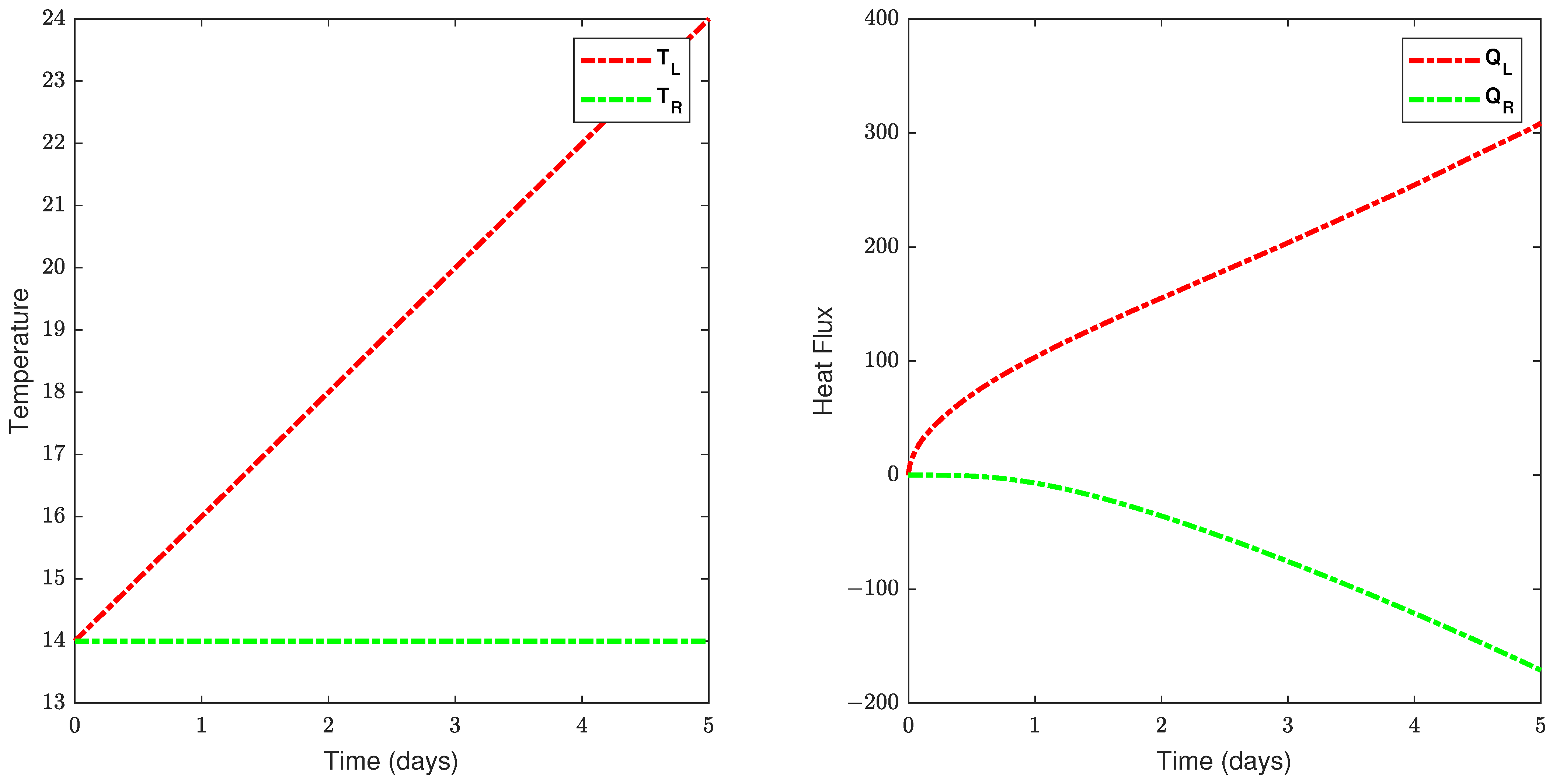
We assume that the boundary temperature and heat flux values are recorded every minute for five days. Therefore, we construct the four time series , , , and by evaluating their corresponding functions at 7200 equally spaced time points. These four time series are grouped to be our Dataset 1 and they are presented in Figure 1.
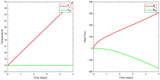
Figure 1.
Plot of the temperature and heat flux at the boundary in Dataset 1.
Optimization Results for Dataset 1
Giving only Dataset 1, our goal now is to estimate the parameters , and . For Approach 1, the implementation is straightforward, as the objective function uses all the boundary data at once for evaluation. On the other hand, Approach 2 requires first estimating the boundary conditions to be used in solving the heat equation. As explained above, we assume Dirichlet boundary conditions and estimate the temperature functions by interpolating the discrete time series . We also estimate the initial condition by means of the polynomial approximation (4). The estimated initial and boundary conditions match the actual conditions in (7). This is expected because the data are free of noise. Finally, to evaluate the objective function , we only need the heat flux time series and choose N.
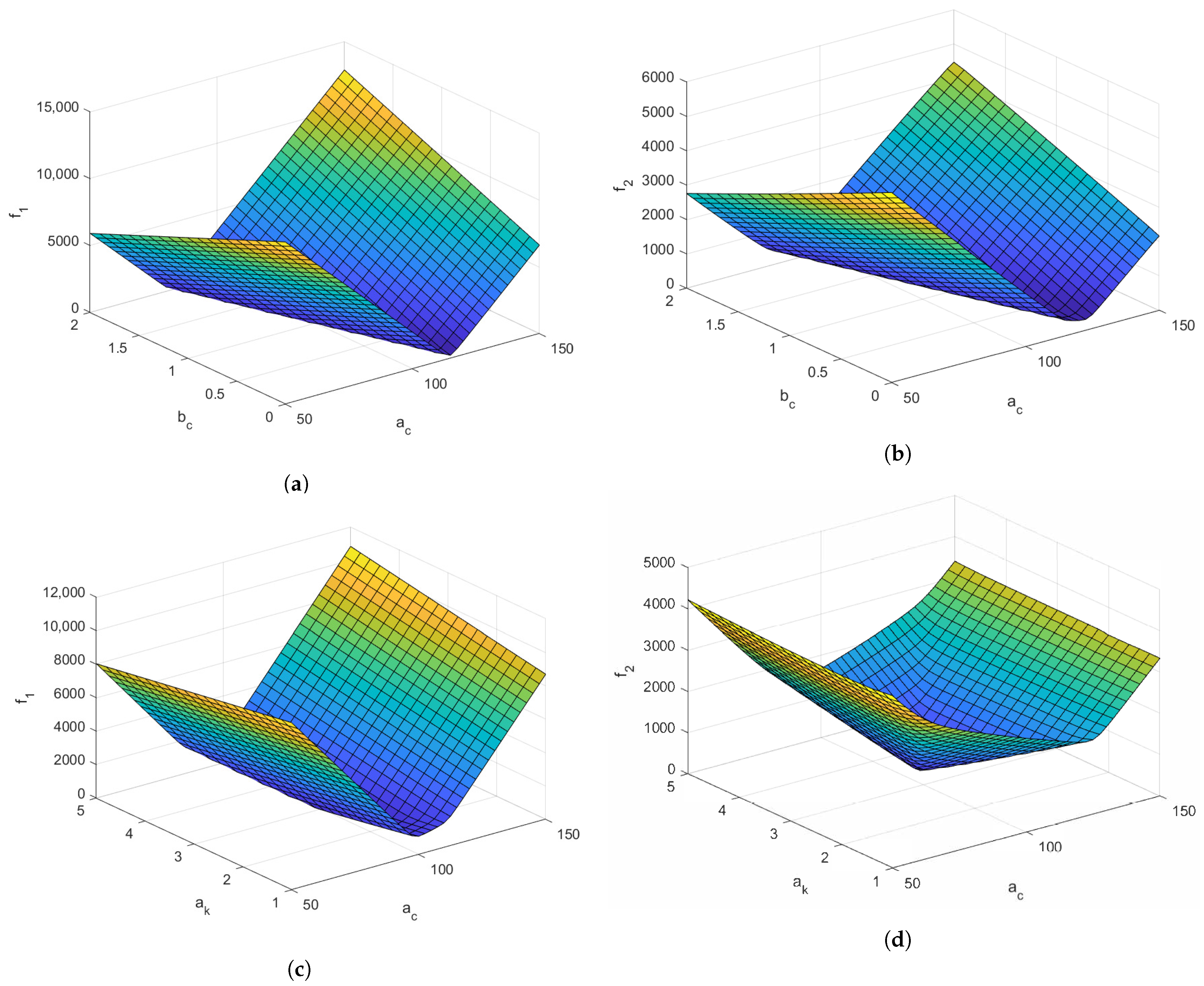
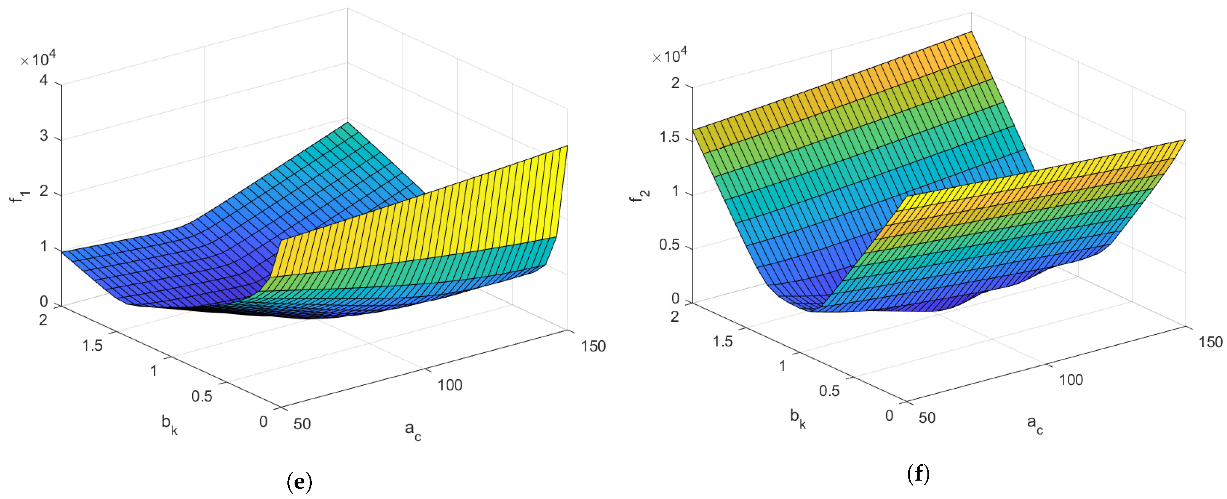
Table 1 shows the optimization results of the two objective functions and using Dataset 1. We refer to the minimum value of the objective function, depending on the approach considered, by . We consider different choices for N in the second objective function, . The data were generated using in the numerical solver, and therefore, this choice for N provides the smallest value for the objective function. Using the recursive optimization strategy, N is found to be 80, and we still obtain a good estimation of all parameters. The parameters estimated through Approach 1 are not accurate but still better than the parameters obtained from Approach 2 with . Furthermore, the time required to minimize is relatively short compared to minimizing . The estimated parameters obtained from Approach 1 are used as an initial guess in the recursive optimization strategy to speed up the process. The behavior of the two objective functions is illustrated in Figure 2. The surface plot of is more concave, which helps to find the global optimum.

Table 1.
The optimization results using Dataset 1, where is the minimum value of or depending on the approach.


Figure 2.
Different plots of (left side) and (right side) using Dataset 1. (a) Plot of for , and varying and . (b) Plot of for , and varying and . (c) Plot of for , and varying and . (d) Plot of for , and varying and . (e) Plot of for , and varying and . (f) Plot of for , and varying and .
3.2. Dataset 2
Dataset 2 is generated in the same procedure as Dataset 1 but with the following initial boundary conditions:
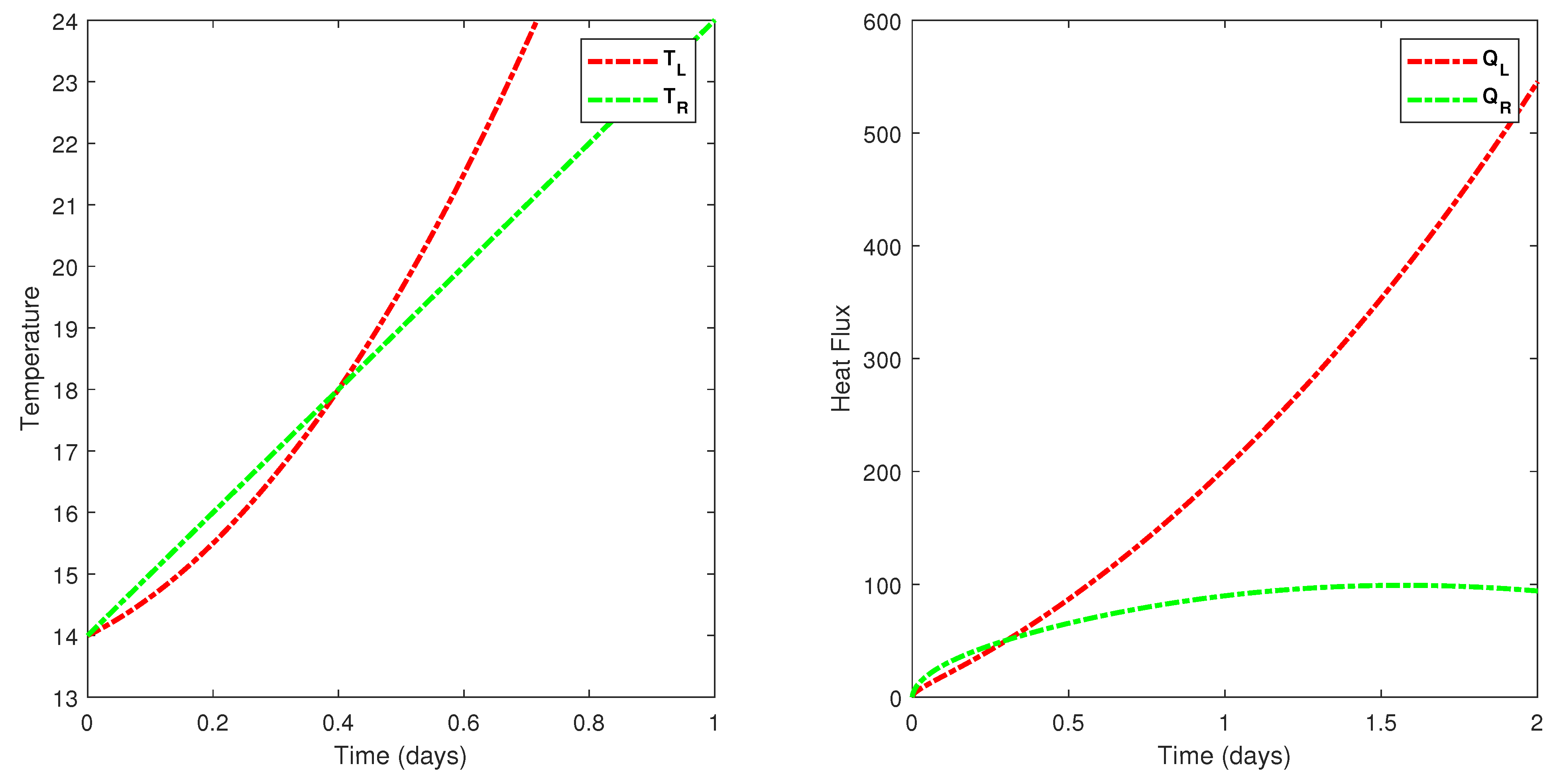
and assuming , and . Temperature and heat flux values are assumed to be recorded every 5 minutes for 10 days. The resulting temperature and heat flux time series are presented in Figure 3. In this case, is less than at the beginning, but then becomes greater than . The efficiency of Approach 1 is expected to degrade in such situations.
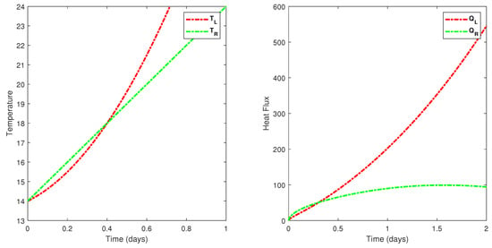
Figure 3.
Plot of the temperature and heat flux at the boundary in Dataset 2.
Optimization Results for Dataset 2
Table 2 shows the optimization results of the two objective functions using Dataset 2. The value of the first objective function is high compared to the results obtained using Dataset 1. The estimated parameters are generally acceptable, especially , which is estimated to be . The objective function, , is minimized with different choices for N and the results started to converge when . We start the recursive optimization strategy with and increase it by 5 in each iteration. The algorithm ends when because the change in is less than .

Table 2.
The optimization results using Dataset 2, where is the minimum value of or depending on the approach.
To visualize the objective functions, we fix at three values which produce the surface graphs in Figure 4 and Figure 5. It can be seen that for both functions as increases, the plotted surfaces flatten in the direction of .

Figure 4.
Different plots of using Dataset 2 with . (a) . (b) . (c) .

Figure 5.
Different plots of using Dataset 2 with . (a) . (b) . (c) .
In the next dataset, we consider oscillating boundary conditions to show the limitation of Approach 1 in such scenarios. On the other hand, Aprroach 2 can handle any boundary conditions, but the computational cost may increase to achieve a certain accuracy.
3.3. Dataset 3
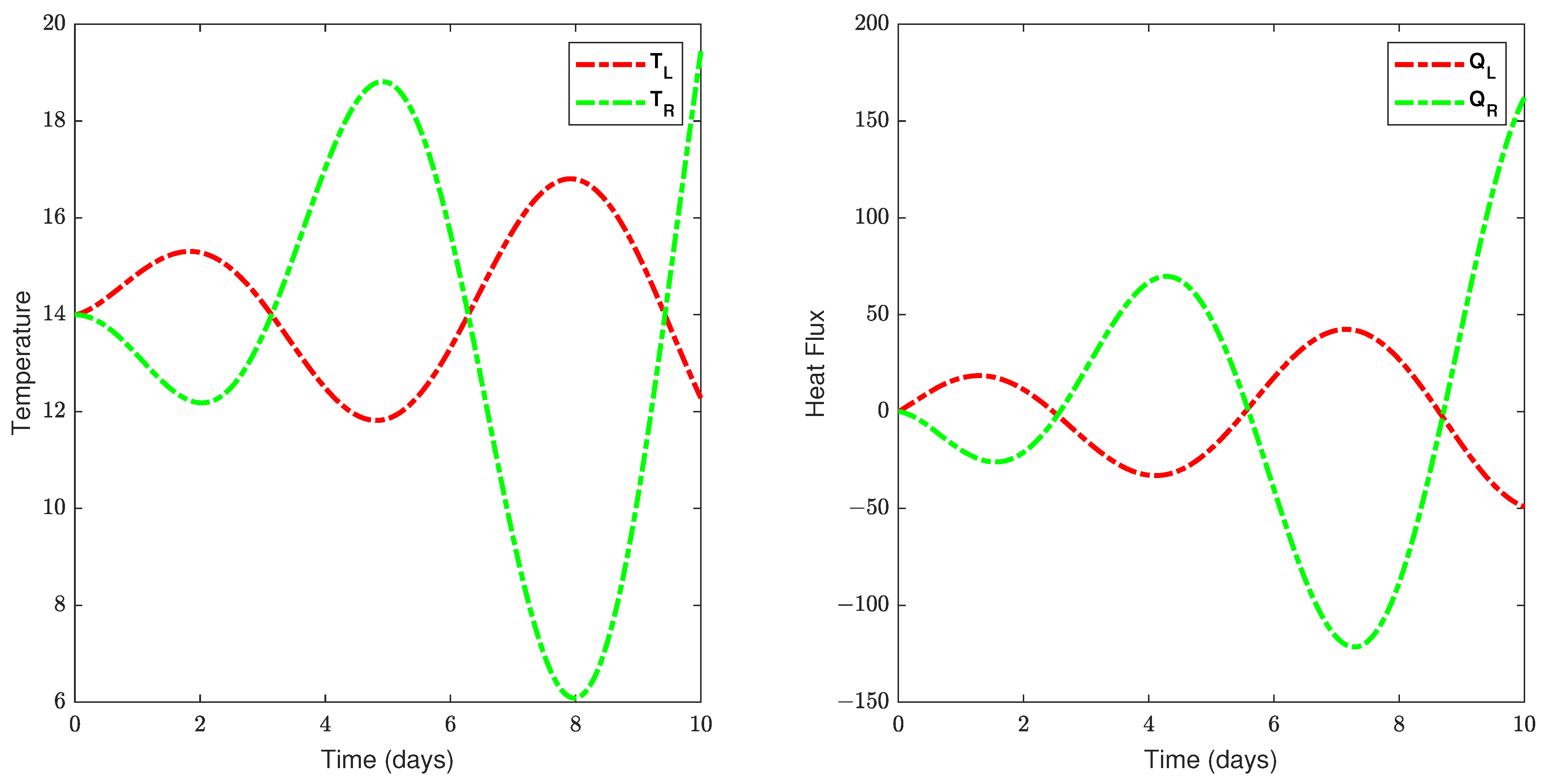
In Datasets 1 and 2, the temperature boundary conditions used to generate data are increasing functions with time. For Dataset 3, more realistic boundary conditions are assumed to create synthetic measurements. The initial and boundary conditions are defined as follows:
The thermal conductivity, K, and heat capacity C are assumed constants by letting . Temperature and heat flux time series are generated over 10 days and assuming that the measurements are recorded every 5 minutes. A visualization of the Dataset 3 time series is provided in Figure 6.
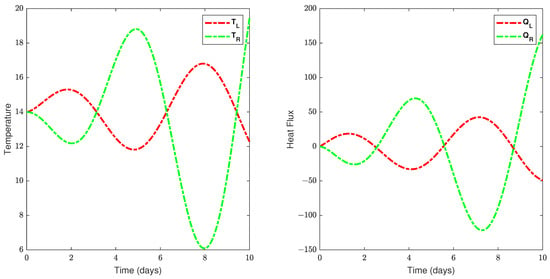
Figure 6.
Plot of the temperature and heat flux at the boundary in Dataset 3.
Optimization Results for Dataset 3
Table 3 shows that the first objective function produces a small error but with false parameter estimates. This is because Approach 1 is not suitable to use with oscillating boundary conditions. Approach 2 gives a high value for the objective function when , but this value decreases significantly with N. The recursive optimization strategy finds a good estimate of the parameters when . The best results are achieved when as expected.

Table 3.
The optimization results using Dataset 3, where is the minimum value of or depending on the approach.
Figure 7 illustrates the shape of the objective functions when . These figures suggest that fixing and to zero can simplify the optimization problem. However, the minimum value for is still far from the true values. The minimum value of is attained at the true parameters.
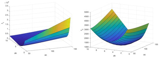
Figure 7.
Plots of and using Dataset 3 with .
4. Uncertainty Quantification
Real measurements are usually corrupted with noise due to the precision of the measuring devices or the experimental setups. In this section, we assume that our measurements of temperature and heat flux at the boundaries are noisy and study how the presence of the noise affects the estimation of the parameters. Noise is assumed to be additive and follows a Gaussian distribution with a mean of zero and a variance of . Therefore, the given boundary measurements are defined by
where and represents the true unknown temperature and heat flux and .
With these assumptions, we need to generalize the deterministic approaches developed earlier to incorporate statistical modeling of the noisy data. In particular, we focus on Approach 2 as it provides more accurate results in the absence of noise. Approach 1 can still be used to obtain a good initial estimate in the optimization strategy.
Using noisy measurements as boundary conditions causes inconsistency in the solution of the heat equation because of the roughness of the boundary data. Therefore, we need to create a smooth representation of the data to be used to solve the forward heat equation. However, this representation is not unique. Assuming we have Dirichlet boundary conditions, we should build multiple smooth temperature functions from the noisy temperature data.
To acomplish that, we first fit an appropriate time series model to the temperature data or use the moving average method to filter the noise from the data, and then we assume and where and are the moving averages or the fitted time series model. From these distributions, we sample and and estimate continuous boundary conditions using smoothing splines. For each pair of estimated smooth temperature functions, we solve the heat equation for a given where the initial condition is approximated by the third-degree polynomial used before. Then, the heat fluxes are computed from the obtained solution.
To find in these settings, we define a likelihood function that is the probability distribution of the heat flux measurements. From the noise assumptions, the likelihood function is given by
Maximizing the likelihood function (12) is equivalent to minimizing the objective function
where and are heat fluxes computed at time using sample j for the boundary conditions.
In this case, we find the maximum-likelihood estimate (MLE) of for each sample of the boundary conditions and . Drawing a set of samples , we obtain the corresponding MLEs of . We summarize our UQ approach in Algorithm 2.
| Algorithm 2 UQ framework |
|
As a special case, if the thermal conductivity and the heat capacity are assumed constants, then the heat equation becomes linear and the effect of the noise in the boundary conditions can be integrated analytically, as shown in [17,18]. The UQLab Matlab toolbox [29] could be utilized to generalize Algorithm 2 to estimate temperature-dependent thermal parameters without assuming a specific functional form for them. In addition, our UQ framework could be extended to sequential filtering following the approach discussed in [30].
In the next section, we reconsider Dataset 1 after adding noise and apply Algorithm 2 to estimate the unknown parameters using the noisy data.
4.1. Numerical Example 1
Noisy data are obtained by adding independent Gaussian random perturbations to the four time series , and from Dataset 1 as in (8) where and . Using deterministic methods results in biased estimates of the parameters as presented in Table 4. Approach 1 works directly given the noisy data, and despite the increased value of the objective function, the estimated parameters are similar to the ones obtained in Table 1. On the other hand, Approach 2 fails when using the noisy data directly as the numerical solver cannot converge with rough boundary conditions. Instead, we construct smooth boundary conditions using moving average and smoothing splines and then maximize the likelihood function (12) or equivalently minimize the objective function (13). In this case, we use to eliminate the effect of the modeling error and study only the noise effect.

Table 4.
The optimization results using noisy Dataset 1, where is the minimum value of or depending on the approach.
Following the UQ framework, we construct two probability distributions:
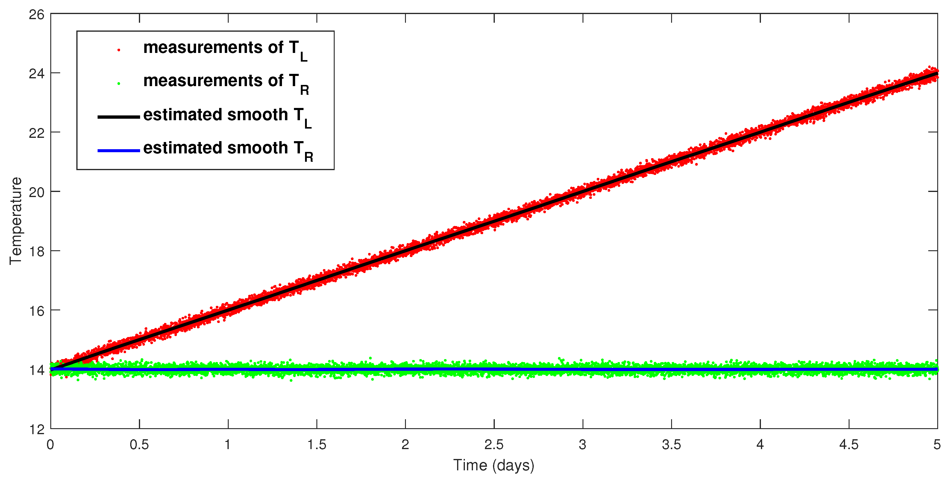
where and are the moving averages of the noisy temperature data. Figure 8 shows one sample of the boundary conditions compared with the noisy data. We draw 50 independent samples of boundary conditions and find the corresponding maximum-likelihood estimate of for each sample. The sample mean and standard deviation are presented in Table 5. In general, the estimated mean is close to the true parameters with small values for the standard deviation. Increasing the sample size would improve the estimates and their confidence levels.

Figure 8.
Plot of one estimated sample of the boundary conditions with the noisy measurements.

Table 5.
Mean and standard deviation of obtained using Algorithm 2 and noisy Dataset 1.
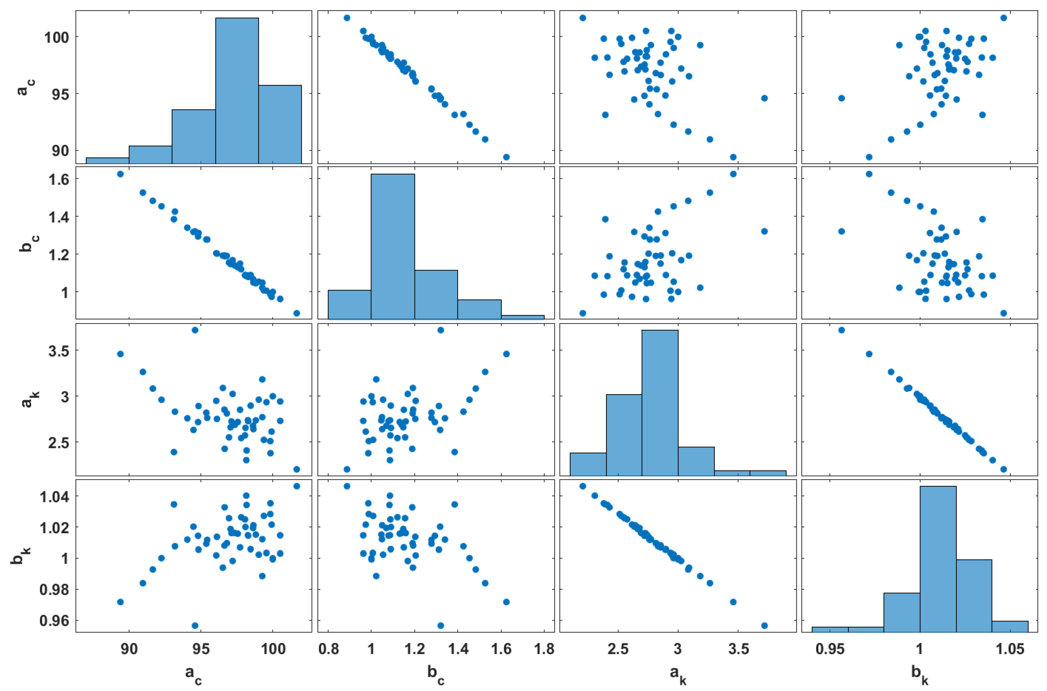
The estimated parameters from Algorithm 2 can be further analyzed by looking at their bivariate correlations. Scatter plots of the 50 samples are presented in Figure 9. The heat capacity parameters, and , are highly correlated. A similar conclusion can be drawn for the thermal conductivity parameters, and . Other combinations of parameters show only moderate correlations. This observation is crucial when making f predictions, as random perturbations of these parameters will not produce realistic physical simulations.
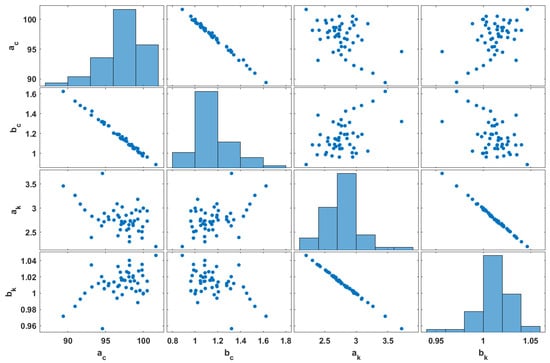
Figure 9.
Scatter plots of the estimated samples of using noisy Dataset 1.
4.2. Numerical Example 2
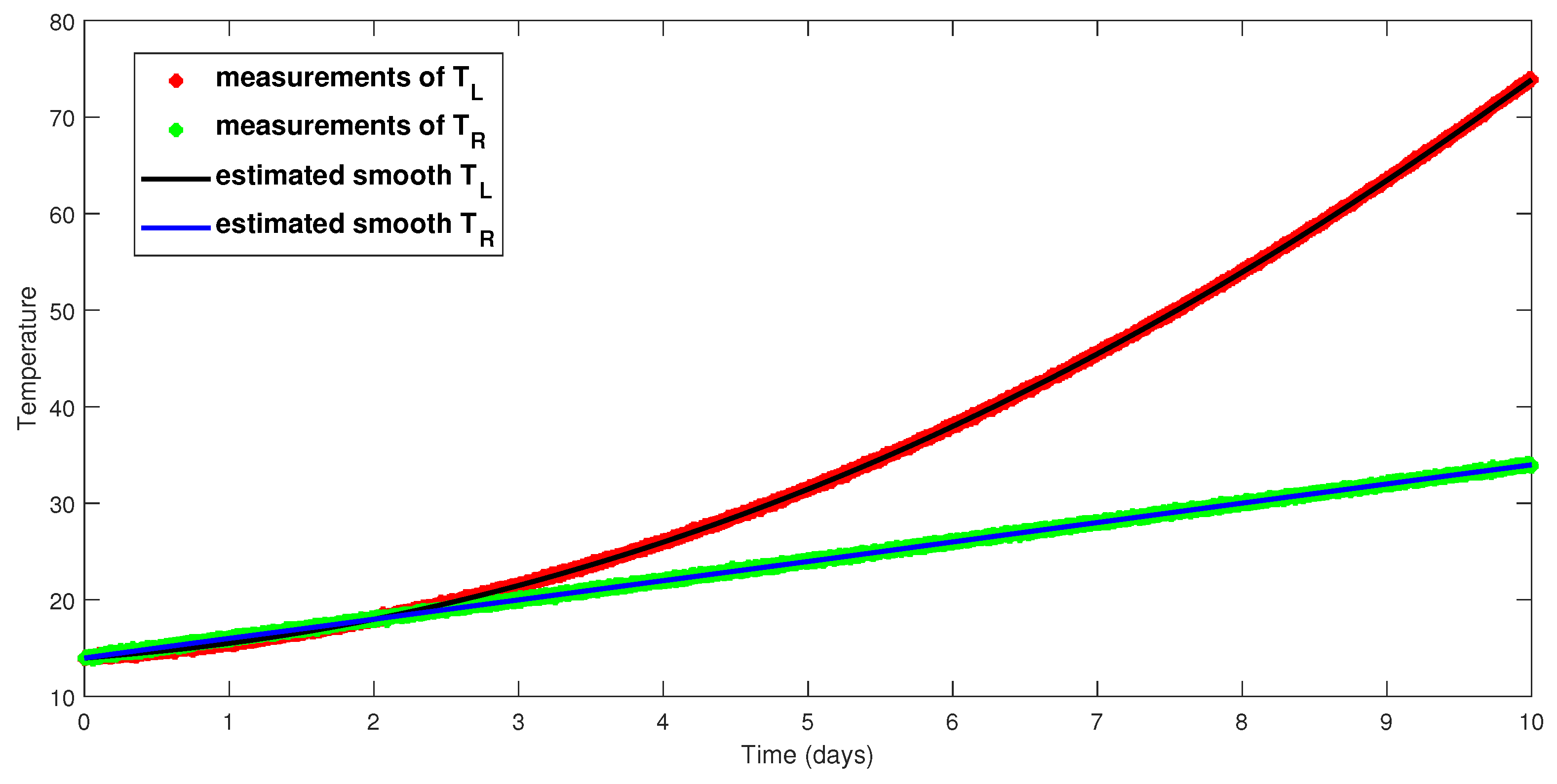
In this example, we add noise to Dataset 2 and apply the UQ framework to estimate the thermal properties. The noisy measueremts are obtained by adding independent Gaussian random perturbations to the four time series , and in Dataset 2 with standard deviations and , respectively. Applying the UQ framework, we employ the noisy temperature data to calculate the probability distribution of the boundary conditions. Figure 10 shows one sample of the boundary conditions compared to the noisy data.
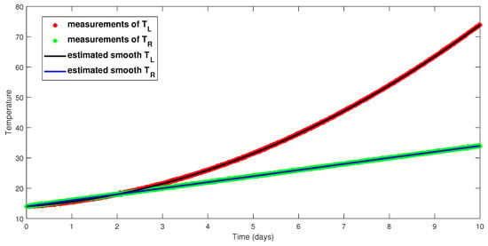
Figure 10.
Plot of one estimated sample of the boundary conditions with the noisy measurements.
Again, we draw 50 independent samples of boundary conditions and find the corresponding maximum-likelihood estimate of for each sample. The sample mean and standard deviation of the maximum-likelihood estimates are presented in Table 6. Scatter plots of the 50 maximum-likelihood estimates obtained using noisy Dataset 2 are presented in Figure 11. This time, all the parameters appear to be highly correlated. One reason for these elevated correlations is the fact that the true value of the parameter is zero and the optimization algorithm is constrained to find positive values for all parameters.

Table 6.
Mean and standard deviation of obtained using Algorithm 2 and noisy Dataset 2.
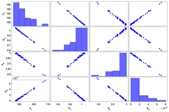
Figure 11.
Scatter plots of the estimated samples of using noisy Dataset 2.
5. Conclusions
In summary, the inverse heat conduction problem in the one-dimensional heat equation with time-dependent temperature and heat flux at both ends was considered. Two methods were developed to estimate the temperature-dependent thermal conductivity and heat capacity, which were assumed to have linear form of the temperature. The first method used an integral approach with a third degree polynomial approximating the temperature, while the second method used a numerical PDE solver and minimized the difference between numerical simulations and measurements.
Multiple datasets were generated using different initial-boundary conditions and thermal coefficients to test the two methods. The results showed that Approach 1 (integral approach) generally required the boundary conditions to be increasing (monotonic) functions, while that was not needed for Approach 2 (numerical approach). The performance of Approach 2 depended on the accuracy of the numerical PDE solver, which was characterized by N. Despite the fact that it took more computational time, Approach 2 yielded better estimates than Approach 1. When N was not large enough, the objective function had rough surfaces, resulting in the presence of many local minimums. Selecting a very large N was computationally expensive and impractical in some cases. Therefore, a recursive optimization strategy was implemented to find the lowest possible value for N that would guarantee a good estimate of the unknown parameters.
In real applications, data are corrupted by noise, and deterministic approaches need to be modified to account for uncertainty. Approach 2 was integrated within an uncertainty quantification framework. The proposed framework was tested with noisy synthetic data. Temperature and heat flux measurements were modeled by independent Gaussian distributions. By sampling the temperature boundary conditions and minimizing the likelihood function given the heat flux measurements, a sampling mechanism for was created. These samples were then used to estimate a complete probability distribution of instead of a single estimate. It was also noticed that the parameters were highly correlated due to their physical nature.
This work demonstrated that estimating temperature-dependent thermal properties in a one-dimensional heat equation is a challenging but feasible task. The proposed methods provided reliable and accurate estimates of the thermal properties under different scenarios and conditions. The uncertainty quantification framework assessed the reliability of estimated parameters and provided useful information for decision making.
Author Contributions
Conceptualization, Z.S.; Methodology, A.S. and Z.S.; Software, A.S. and Z.S.; Validation, Z.S.; Formal analysis, Z.S.; Investigation, A.S.; Resources, A.S. and Z.S.; Writing—original draft, A.S. and Z.S.; Writing—review & editing, Z.S.; Supervision, Z.S. All authors have read and agreed to the published version of the manuscript.
Funding
This research received no external funding.
Data Availability Statement
Data sharing not applicable.
Acknowledgments
This paper is based upon work supported by King Fahd University of Petroleum & Minerals and the authors acknowledge the support.
Conflicts of Interest
The authors declare no conflict of interest.
References
- Woodbury, K.A.; Najafi, H.; De Monte, F.; Beck, J.V. Inverse Heat Conduction: Ill-Posed Problems; John Wiley & Sons, Incorporated: Hoboken, NJ, USA, 2023. [Google Scholar]
- Roy, A.D.; Dhiman, S. Solutions of One-Dimensional Inverse Heat Conduction Problems: A Review; Transactions of the Canadian Society for Mechanical Engineering: Ottawa, ON, Canada, 2023. [Google Scholar]
- Orlande, H.R. Inverse problems in heat transfer: New trends on solution methodologies and applications. J. Heat Transf. 2012, 134, 031011. [Google Scholar] [CrossRef]
- François, A.; Ibos, L.; Feuillet, V.; Meulemans, J. Estimation of the thermal resistance of a building wall with inverse techniques based on rapid active in situ measurements and white-box or ARX black-box models. Energy Build. 2020, 226, 110346. [Google Scholar] [CrossRef]
- Biddulph, P.; Gori, V.; Elwell, C.A.; Scott, C.; Rye, C.; Lowe, R.; Oreszczyn, T. Inferring the thermal resistance and effective thermal mass of a wall using frequent temperature and heat flux measurements. Energy Build. 2014, 78, 10–16. [Google Scholar] [CrossRef]
- Sassine, E.; Cherif, Y.; Antczak, E. Parametric identification of thermophysical properties in masonry walls of buildings. J. Build. Eng. 2019, 25, 100801. [Google Scholar] [CrossRef]
- Kim, S.; Kim, M.C.; Kim, K.Y. An integral approach to the inverse estimation of temperature-dependent thermal conductivity without internal measurements. Int. Commun. Heat Mass Transf. 2002, 29, 107–113. [Google Scholar] [CrossRef]
- Kim, S.; Chung, B.J.; Kim, M.C.; Kim, K.Y. Inverse estimation of temperature-dependent thermal conductivity and heat capacity per unit volume with the direct integration approach. Numer. Heat Transf. Part A Appl. 2003, 44, 521–535. [Google Scholar] [CrossRef]
- Kim, S.; Lee, K.J.; Ko, Y.J.; Kim, M.C.; Kim, K.Y. Estimation of temperature-dependent thermal conductivity and heat capacity per unit volume with a simple integral approach. Int. Commun. Heat Mass Transf. 2004, 31, 981–990. [Google Scholar] [CrossRef]
- Ngo, T.; Huang, J.; Wang, C. Inverse simulation and experimental verification of temperature-dependent thermophysical properties. Int. Commun. Heat Mass Transf. 2016, 71, 137–147. [Google Scholar] [CrossRef]
- Hussein, M.S.; Lesnic, D.; Ivanchov, M.I. Simultaneous determination of time-dependent coefficients in the heat equation. Comput. Math. Appl. 2014, 67, 1065–1091. [Google Scholar] [CrossRef]
- Chen, H.; Lin, J. Simultaneous estimations of temperature-dependent thermal conductivity and heat capacity. Int. J. Heat Mass Transf. 1998, 41, 2237–2244. [Google Scholar] [CrossRef]
- Huang, C.; Jan-Yuan, Y. An inverse problem in simultaneously measuring temperature-dependent thermal conductivity and heat capacity. Int. J. Heat Mass Transf. 1995, 38, 3433–3441. [Google Scholar] [CrossRef]
- Parthasarathy, S.; Balaji, C. Estimation of parameters in multi-mode heat transfer problems using Bayesian inference–Effect of noise and a priori. Int. J. Heat Mass Transf. 2008, 51, 2313–2334. [Google Scholar] [CrossRef]
- Gnanasekaran, N.; Balaji, C. A Bayesian approach for the simultaneous estimation of surface heat transfer coefficient and thermal conductivity from steady state experiments on fins. Int. J. Heat Mass Transf. 2011, 54, 3060–3068. [Google Scholar] [CrossRef]
- Kaipio, J.P.; Fox, C. The Bayesian framework for inverse problems in heat transfer. Heat Transf. Eng. 2011, 32, 718–753. [Google Scholar] [CrossRef]
- Ruggeri, F.; Sawlan, Z.; Scavino, M.; Tempone, R. A hierarchical Bayesian setting for an inverse problem in linear parabolic PDEs with noisy boundary conditions. Bayesian Anal. 2017, 12, 407–433. [Google Scholar] [CrossRef]
- Iglesias, M.; Sawlan, Z.; Scavino, M.; Tempone, R.; Wood, C. Bayesian inferences of the thermal properties of a wall using temperature and heat flux measurements. Int. J. Heat Mass Transf. 2018, 116, 417–431. [Google Scholar] [CrossRef]
- Alifanov, O.M. Inverse Heat Transfer Problems; Springer Science & Business Media: Berlin/Heidelberg, Germany, 2012. [Google Scholar]
- Ozisik, M.N. Inverse Heat Transfer: Fundamentals and Applications; Routledge: Abingdon, UK, 2018. [Google Scholar]
- Lesnic, D. Inverse Problems with Applications in Science and Engineering; CRC Press: Boca Raton, FL, USA, 2021. [Google Scholar]
- Kaipio, J.; Somersalo, E. Statistical and Computational Inverse Problems; Springer Science & Business Media: Berlin/Heidelberg, Germany, 2006; Volume 160. [Google Scholar]
- Skeel, R.D.; Berzins, M. A method for the spatial discretization of parabolic equations in one space variable. SIAM J. Sci. Stat. Comput. 1990, 11, 1–32. [Google Scholar] [CrossRef]
- Craven, P.; Wahba, G. Smoothing noisy data with spline functions. Numer. Math. 1978, 31, 377–403. [Google Scholar] [CrossRef]
- Broyden, C.G. The Convergence of a Class of Double-Rank Minimization Algorithms. J. Inst. Math. Applic. 1970, 6, 76–90. [Google Scholar] [CrossRef]
- Fletcher, R. A New Approach to Variable Metric Algorithms. Comput. J. 1970, 13, 317–322. [Google Scholar] [CrossRef]
- Goldfarb, D. A Family of Variable Metric Updates Derived by Variational Means. Math. Comput. 1970, 24, 23–26. [Google Scholar] [CrossRef]
- Shanno, D.F. Conditioning of Quasi-Newton Methods for Function Minimization. Math. Comput. 1970, 24, 647–656. [Google Scholar] [CrossRef]
- Marelli, S.; Sudret, B. UQLab: A framework for uncertainty quantification in Matlab. In Vulnerability, Uncertainty, and Risk: Quantification, Mitigation, and Management; American Society of Civil Engineers: Reston, VS, USA, 2014; pp. 2554–2563. [Google Scholar]
- Iglesias, M.; Sawlan, Z.; Scavino, M.; Tempone, R.; Wood, C. Ensemble-marginalized Kalman filter for linear time-dependent PDEs with noisy boundary conditions: Application to heat transfer in building walls. Inverse Probl. 2018, 34, 075002. [Google Scholar] [CrossRef]
Disclaimer/Publisher’s Note: The statements, opinions and data contained in all publications are solely those of the individual author(s) and contributor(s) and not of MDPI and/or the editor(s). MDPI and/or the editor(s) disclaim responsibility for any injury to people or property resulting from any ideas, methods, instructions or products referred to in the content. |
© 2023 by the authors. Licensee MDPI, Basel, Switzerland. This article is an open access article distributed under the terms and conditions of the Creative Commons Attribution (CC BY) license (https://creativecommons.org/licenses/by/4.0/).

