LSTM Reconstruction of Turbulent Pressure Fluctuation Signals

Abstract

This paper concerns the application of a long short-term memory model (LSTM) for high-resolution reconstruction of turbulent pressure fluctuation signals from sparse (reduced) data. The model’s training was performed using data from high-resolution computational fluid dynamics (CFD) simulations of high-speed turbulent boundary layers over a flat panel. During the preprocessing stage, we employed cubic spline functions to increase the fidelity of the sparse signals and subsequently fed them to the LSTM model for a precise reconstruction. We evaluated our reconstruction method with the root mean squared error (RMSE) metric and via inspection of power spectrum plots. Our study reveals that the model achieved a precise high-resolution reconstruction of the training signal and could be transferred to new unseen signals of a similar nature with extremely high success. The numerical simulations show promising results for complex turbulent signals, which may be experimentally or computationally produced.

1. Introduction

Machine learning (ML) has become a popular tool for analyzing time series data in diverse applications, including engineering, medical science, finance, and sensor data analysis [1]. Its applications on time series data can include forecasting, classification, and reconstruction of the original signal using incomplete or noisy samples. For example, researchers inferred and classified possible cardiac pathologies based on time series data collected from a 24 h Holter recording [2]. In other studies, long short-term memory (LSTM) [3] and bidirectional LSTM models were employed to forecast stock market prices [4,5].

ML techniques were used for signal reconstruction tasks to recover the original signal from noisy or incomplete data. Stacked denoising autoencoders were used in [6] to recover compressed electrocardiogram signals during fetal electrocardiogram monitoring. In a similar framework, the authors of [7] proposed a Doppler sensor-based ECG signal reconstruction method using a hybrid deep learning (DL) model with a convolutional neural network (CNN) and LSTM. LSTM networks were also employed to interpolate air pollutant concentrations [8] and in conjunction with a CNN to reconstruct three-dimensional turbulent channel flows [9]. Image super resolution-based machine learning techniques have also been considered to recover grossly coarse spatiotemporal flow data back to a high resolution [10].

More recently, DL techniques such as CNNs were used to reconstruct turbulent flows [11], which is a highly complex and nonlinear phenomenon. Variations of CNN models were tested for the reconstruction of the flow field in supersonic combustors [12] and the reconstruction of laminar flow from low-resolution flow field data [13]. Our study focuses on a high-fidelity reconstruction of turbulent pressure fluctuations from coarse or coarse-grained data using LSTM networks and a granularity-increase preprocessing step. We have investigated pressure time series reconstruction and their power spectra. Power spectra are important for structural mechanics (e.g., acoustic fatigue on structures affected by low-frequency oscillations [14,15]) and fluid mechanics (e.g., boundary layers and turbulence near the wall [16]).

Recently, for a range of DL models, it was shown that missing values and sparse datasets could severely degrade the performance of ML methods [17,18]. Past works attempted to tackle the problem of missing values in time series data. Common techniques include constant value imputation (e.g., zero value, mean value, random value substitution, and missing value prediction with interpolation or ML methods). LSTM networks were used to impute the missing values of plant stem moisture-monitored data [19], while the authors of [20] used wavelet variance analysis to analyze time series with missing values. Preprocessing of time series data to increase fidelity was investigated by the authors of [21], using interpolation to increase the granularity of time series data and forecast stock market indices. Researchers also used fractal interpolation [22,23] to generate a finer time series from insufficient data sets.

The motivation for the present study arises from high-speed (Mach 6) boundary layers over surfaces, where aerodynamic loading will significantly influence the structural response and deformation. In particular, turbulent pressure fluctuations lead to near-wall acoustic effects that can potentially lead to acoustic fatigue. These fluctuations depend on the nature of the boundary layer and manifest differently regarding frequency and amplitudes at very high Mach numbers (e.g., Mach 6) compared with supersonic speeds [24]. Thus, the present study focuses on investigating the ability of DL to reconstruct acoustic signals at Mach 6 and give insight into the applicability of ML methods to a more extreme flow environment compared with the supersonic flow considered previously [18].

ML models for determining aero-structural response at such high speeds have yet to be developed and applied. DL and ML models can potentially use coarse-grain data to reconstruct fine-resolution data. Understanding the behavior of DL and ML models under different sparsity conditions is paramount for using these models in practice. The original fine-grain signals are made sparse to mimic coarse-grained experimental or numerical samples. The reconstruction approach is based on LSTM in conjunction with cubic spline functions during the preprocessing stage to increase the data’s fidelity. The original fine-grained signals derived from high-resolution computational fluid dynamics simulations are used as the gold standard (i.e., “ground truth”) to evaluate and assess the LSTM model’s prediction accuracy.

2. Data Curation

The data used in the present study were obtained from the direct numerical simulations (DNS) in [25]. They concern a flow over a flat plate at Mach 6 subjected to von Kármán atmospheric perturbations at the inlet, with a turbulence intensity for the freestream velocity equal to 1%. The DNS aimed to capture the smallest possible turbulent scales and their associated acoustic loading near-wall effects. The sole purpose of the (atmosphere-like) perturbations was to excite the transition to turbulence of the developing boundary layer in a “natural”-like manner. To avoid bypass transition, a relatively low amplitude was chosen. However, only the pressure signal extracted from probes located on the wall’s surface within the fully developed turbulent boundary layer are considered herein.

2.1. Governing Equations

The compressible Navier–Stokes equations (NSEs) for an ideal gas are solved using the finite volume method (FVM). In the integral form, the NSEs are formulated as follows:

$$\begin{array}{cc}\hfill \frac{\partial }{\partial t}\underset{V}{\iiint }\rho \mathrm{dV}=& -\underset{A}{∯}\rho \left(\overrightarrow{u}·\widehat{n}\right)\mathrm{dA}\hfill \end{array}$$

(1)

$$\frac{\partial }{\partial t}\underset{V}{\iiint }\rho \overrightarrow{u}\mathrm{dV}=-\underset{A}{∯}\left[\rho \overrightarrow{u}\overrightarrow{u}+p\overrightarrow{\overrightarrow{\mathrm{I}}}-\overrightarrow{\overrightarrow{\tau }}\right]·\widehat{n}\mathrm{dA}$$

(2)

$$\frac{\partial }{\partial t}\underset{V}{\iiint }\rho e_t\mathrm{dV}=-\underset{A}{∯}\left[\rho e_t\left(\overrightarrow{u}·\widehat{n}\right)+p\overrightarrow{u}-\left(\overrightarrow{u}·\overrightarrow{\overrightarrow{\tau }}\right)+\overrightarrow{q}\right]·\widehat{n}\mathrm{dA}$$

(3)

where $\rho$ is the density; $\overrightarrow{u}$ is the velocity vector; p is the static pressure; $\widehat{n}$ is the outward pointing unit normal of a surface element $\mathrm{dA}$ of the closed finite control volume $\mathrm{dV}$; $e_t$ is the total energy per unit mass given by $e_t=e+\overrightarrow{u}·\overrightarrow{u}/2$; and e is the specific internal energy, which for a calorically perfect gas is given by

$$\begin{array}{c}e=c_{v}T=\frac{p}{\rho \left(\gamma -1\right)}\end{array}$$

Here, T is the temperature, $c_v$ is the specific heat capacity at a constant volume, and $\gamma$ is the heat capacity ratio (or adiabatic index) defined as $\gamma =c_p/c_v$, where $c_p$ is the specific heat capacity at a constant pressure and $R_s=c_p-c_v=c_v\left(\gamma -1\right)$ is the specific gas constant.

For a Newtonian fluid, the shear stress tensor is given by

$$\overrightarrow{\overrightarrow{\tau }}={\lambda }_b\left(\nabla ·\overrightarrow{u}\right)\overrightarrow{\overrightarrow{\mathrm{I}}}+\mu \left[\nabla \otimes \overrightarrow{u}+{\left(\nabla \otimes \overrightarrow{u}\right)}^T\right]$$

where $\overrightarrow{\overrightarrow{\mathrm{I}}}$ is the identity tensor; the bulk viscosity is given by ${\lambda }_b=-2\mu /3$ according to Stokes’ hypothesis; and $\mu$ is the dynamic viscosity obtained by Sutherland’s law as follows:

$$\begin{array}{c}\mu \left(T\right)={\mu }_{ref}{\left(\frac{T}{T_{ref}}\right)}^{\frac{3}{2}}\frac{T_{ref}+T_s}{T+T_s}\end{array}$$

(4)

where the freestream values are used as the reference and the Sutherland temperature is $T_s=110.4$ K.

The heat flux is calculated by Fourier’s law of heat conduction:

$$\overrightarrow{q}=-\kappa \nabla T$$

where $\kappa$ is the heat conductivity given by

$$\kappa \left(T\right)=\frac{c_p}{\mathrm{Pr}}\mu \left(T\right)$$

and $\mathrm{Pr}=0.72$ is Prandtl’s number.

2.2. Numerical Implementation

We employed the ILES approach in the framework of the in-house block-structured mesh code CNS3D [26,27,28] that solves the full Navier–Stokes equations using a finite volume Godunov-type method for the convective terms, whose inter-cell numerical fluxes are calculated by solving the Riemann problem using the reconstructed values of the primitive variables at the cell interfaces. A one-dimensional swept unidirectional stencil was used in conjunction with a modified variant [28] of the 11th order weighted essentially non-oscillatory (WENO) scheme [29] for reconstruction. The Riemann problem was solved using the so-called “Harten, Lax, van Leer, and (the missing) Contact” (HLLC) approximate Riemann solver [30,31]. The viscous terms were discretized using a second-order central scheme. The solution was advanced in time using a five-stage (fourth-order accurate) optimal strong stability-preserving Runge–Kutta method [32].

Based on the freestream properties (

Table 1. Flow properties for $M_{\infty }=6$.

${\mathit{x}}_{\mathit{l}}$ (mm)	${\mathit{U}}_{\mathit{\infty }}$ (m/s)	${\mathit{T}}_{\mathit{\infty }}$ (K)	${\mathit{p}}_{\mathit{\infty }}$ (kPa)	${\mathsf{\rho }}_{\mathit{\infty }}$ (kg/m3)	${\mathit{T}}_{\mathit{w}}$ (K)	Tu (%${\mathit{U}}_{\mathit{\infty }}$)	${\mathit{Re}}_{\mathit{xl}}$
2.0	1769.92	19.417	216.64	0.3124	1600	1.0	77,791

) and the reference length $x_l=2$ mm, the incoming flow had a Reynolds number of $R{e}_{xl}\simeq 77,800$. The reference length was calculated from the leading edge of the plate. We implemented periodic boundary conditions in the spanwise direction (z). In the wall-normal direction (y), a no-slip isothermal wall (with a temperature $T_w$ of 1600 K, which is near the adiabatic value) was implemented. Finally, the supersonic outflow condition (linear extrapolation) was applied at the outlet and far-field boundaries.

The domain comprised almost $1\times {10}^9$ cells ($4055\times 205\times 605$). The mesh cell size was kept equidistant in the streamwise (x) and spanwise (z) directions, while clustering was employed in the wall-normal (y) direction. The size of the cells was $\Delta x^{+}\simeq 2.25$ and $\Delta z^{+}0.9$ while close to the wall $\Delta y_w^{+}\simeq 0.16$ and at the boundary layer edge $\Delta y_e^{+}\simeq 1.89$.

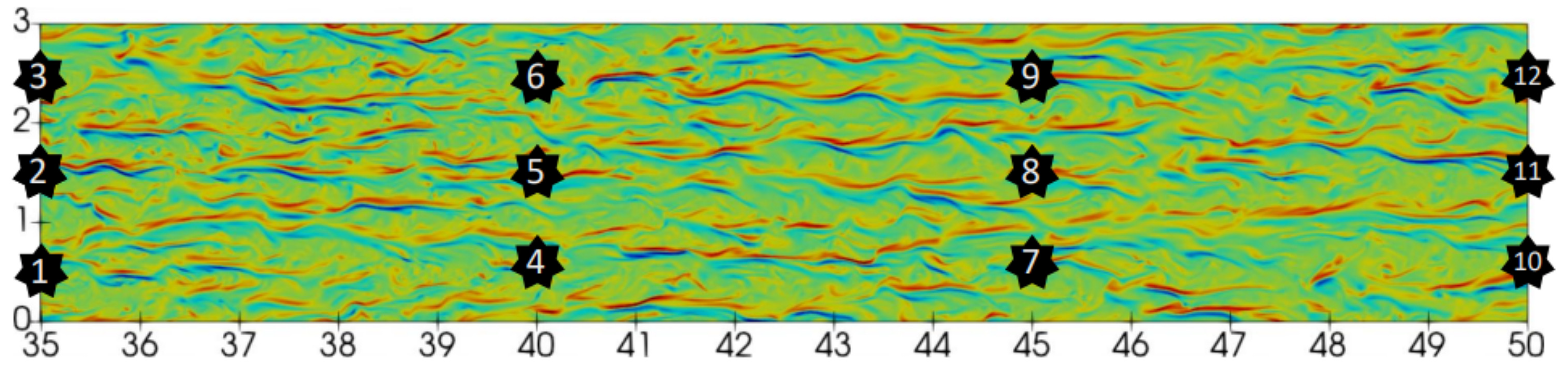
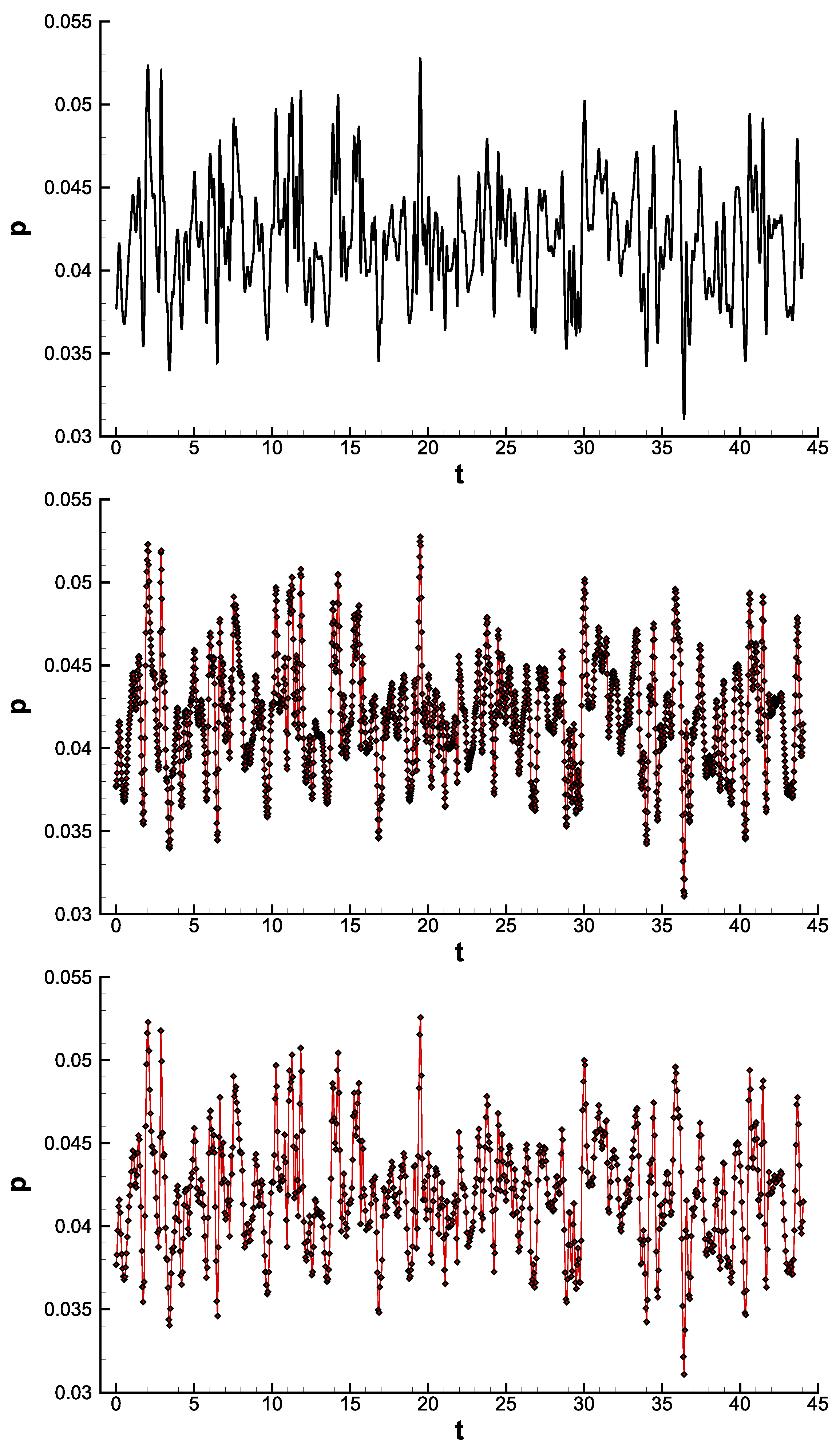
2.3. Pressure Signal Data

This study considered the turbulent flow pressure fluctuations applied on the wall’s surface as a time series over 12 probe positions and 86,098 time steps. The probes’ positions used in the CFD simulations are shown in Figure 1. The CFD simulation produced results for 12 different spatial points on the panel.

All probes were positioned on the wall’s surface ($y=0$) and were equidistant both in the streamwise (x) and spanwise (z) directions (i.e., at fixed intervals of 5 and 1 length units (normalized by the reference length $x_l=2$ mm)), respectively, as per Figure 1. Note that the inflow was prescribed a uniform flowfield superimposed with von Kármán-like atmospheric perturbations with a turbulence intensity equal to 1% of the freestream velocity. The transition occurred between $x\in \left[5,25\right]x_l$, and the flow became fully turbulent by $x\simeq 30$. Thus, all probes were located within the fully turbulent boundary layer (TBL) region. The periodic boundary condition employed in the spanwise direction and the planar wall surface ensured that the turbulence signals between the three probes in the same streamwise direction were statistically homogeneous. In the streamwise direction, the TBL gradually grew, and thus the turbulence statistics became increasingly dissimilar relative to the training probe (number 2). The latter can be corroborated, for example, by the changes in the pressure signal power spectrum shown later in Section 4.2.

Temporally, the signals were sampled over a period of $\simeq 287$ dimensionless time units (i.e., the dimensional time ($t^{*}$) was normalized by $U_{\infty }/{\delta }_{x_{45}}$, where ${\delta }_{x_{45}}\simeq 1.528$ mm is the mean boundary layer height $\delta$ at $x=45x_l$). The number of samples per dimensionless unit time was $\approx 600$. The dimensionless time t is shown in all subsequent plots and defined as $t=t^{*}{U}_{\infty }/{\delta }_{x_{45}}$. The frequency obtained using the dimensionless time is thus the Strouhal number (i.e., $St\equiv f=f^{*}{\delta }_{x_{45}}/U_{\infty }$).

The LSTM model was trained to reconstruct the pressure fluctuation time series corresponding to probe number 2 (see Figure 1). The model was subsequently transferred to all other flat panel probes to reconstruct all results derived by the CFD simulation.

The whole purpose of the method was to reproduce the fine-grained signal from the coarse-grained samples. During training, we only used sparse versions of the original signal. However, we employed splines (see discussion below) as a preprocessing step to increase the fidelity of the sparse signal, resulting in a more fine-grained signal, which we aimed to correct through LSTM.

Figure 2 visualizes the original fine-grained signal and its sparse, coarse-grained versions. Precise high-resolution reconstruction with the minimum mean squared error of the fine-grained signal and precise reconstruction of the power spectrum is the main focus of this study.

To test the limits of our reconstruction methods, we artificially created sparse versions by linearly sampling the data with a predefined stride. We sampled the original fine-grained signal with multiple sparsity factors (i.e., the sample step) in the range of [2, 100]. For reference, at a sparsity level of $k=40$, only 2152 sample points were available for training the model, with the remaining 83,946 points left to be interpolated. Note that 86,098-time samples were available in the original signal produced by the CFD. Since we used the sparse signal versions, for the case of a sparsity factor of 40, we only sampled 2152 points from the original signal. Thus, 83,946 (86,098 − 2152) unsampled points were the ones we tried to predict through our method to reproduce the original CFD time series.

In Figure 2, the x axis depicts time normalized by ${\delta }_0/u_{\infty }$. At the same time, the y axis represents the pressure fluctuation normalized by $q_{\infty }=\gamma p_{\infty }{M}^2/2$, where the subscript ${(}_{\infty })$ designates the freestream properties, ${\delta }_0$ is the boundary layer height at the inlet, and $\gamma =1.4$ is the adiabatic index for air. The original signal, shown on top, comprises 86,098 time samples. The second signal (sparsity = 40) contained 2152 time samples. The signal at the bottom (sparsity = 100) contained only 861 samples. Only sparse versions of the signal were used for training the LSTM model. The original signal served as the target for evaluating the reconstruction error.

The sample size of the pressure signals was sufficient to resolve all fluctuation modes in the present turbulent flow case. The pressure power spectrum plots in Section 4.2 suggest that the ground truth signals’ low- and high-frequency pressure regions were adequately resolved, as inferred by the well-defined energy-containing and sub-inertial ranges. Training the LSTM model using smaller subsets of the considered data set showed that the present results were not affected by overfitting. The results of training the DL model using smaller signal subsets were thus omitted for brevity.

3. LSTM

Recurrent neural networks (RNNs), such as the long-short-term memory (LSTM) network model [3], have been previously applied to time series forecasting [33,34,35]. However, the use of LSTM for aeroelastic and aeroacoustic applications is scarce. It was previously utilized in conjunction with proper orthogonal decomposition (POD) to establish the relationship between the velocity signals of discrete points [36] and the time-varying POD coefficients and reconstruct the downstream pressure by using the upstream pressure as input [37]. Applying forecasting methods such as LSTM in fluid mechanics and acoustics problems is an emerging research field.

Past application of LSTM for supersonic flows showed that the model could effectively capture the temporal dependencies in the data [18]. However, technical challenges arise when LSTM networks are used to interpolate intermediate values and reconstruct fine-grained signals from sparse time series. This is particularly true for signals containing large amplitudes within extremely short intervals, like the Mach 6 turbulent flow over a panel. The missing values in the input sequence are large, and possibly differing the $dt$ time sampling between samples must be addressed. A high-level schematic of the present LSTM network architecture is shown in Figure 3.

LSTM networks consume sequential data. Ideally, the time sample between all subsequent values is constant and equal to the time step size $dt$. During the reconstruction phase (i.e., the testing phase), we must use $d{t}_{\mathrm{test}}=dt$ to ensure that all sample points are predicted (interpolated). The model’s training must adhere to this limitation if we want accurate predictions of the next sample over $dt$.

However, missing (intermediate) values present in sparse signals do not allow for this, since subsequent samples have a distance of $d{t}_{\mathrm{train}}=k$ × $dt>dt$. Hence, the model’s output corresponds to a sample k time steps ahead, omitting unknown intermediate samples. Given an input sequence of N points spanning over N × $d{t}_{\mathrm{train}}$ time units, the model’s output corresponds to the sample at time $(N+1)d{t}_{\mathrm{train}}$.

The different $dt$ value used between training and testing poses an important problem since the objectives differ. To overcome this limitation, we employed a missing value imputation preprocessing step for the sparse time series similar to the application in [21,23].

Hence, during training and testing, we enforced $d{t}_{\mathrm{train}}=d{t}_{\mathrm{test}}=dt$ by imputing missing intermediate values in the sampled sparse signals via cubic spline functions, increasing their fidelity. This rendered both the training and testing sequences suitable for the LSTM network and high-fidelity signal reconstruction:

$$P\{t+1\}=\mathrm{LSTM}\left([S_{t-\ell },F\left(S_{t-\ell +1}\right),\dots ,S_{t-\frac{\ell }{2}+1},\dots ,F\left(S_t\right)]\right)$$

(5)

where P denotes the output prediction of the model, $S_k$ denotes the $k_{th}$ element of the input sequence S, $F\left(S_k\right)$ denotes imputed values through a cubic spline function F, ℓ denotes the length of the input sequence, and brackets $\left[\right]$ denote a sequence.

We adjusted the input sequence length ℓ to ℓ$=2$ × $sparsity\_factor$. This ensured that every input sequence during testing would consist of two experimental samples, and the rest were the imputed values. We experimented with various lengths ℓ$=m$ × $sparsity\_factor$ and found that $m=2$ worked well.

During our study, we also tested other common methods of missing value imputation, like zero-filling and mean value imputation [38]. Still, the results were suboptimal compared with imputation via cubic splines. Cubic spline interpolation provided a much more accurate initial guess for the missing sparsed signal points than just using the simpler zero-padding or constant mean value. Conversely, more complex interpolation schemes (e.g., high-order polynomials, B-spline interpolation, or nonuniform fast Fourier transform (NUFFT) with a B-spline basis [39,40]) may help improve the results, but this remains to be examined. The spline function artificially increases the available data. At the same time, LSTM provides robustness against random noise and greater generalizability, which splines have been shown to suffer from [17].

Training and Model Hyperparameters

Only probe 2 was used as a training data set, with the remaining points unseen and only used as a test set. Before training, we split the available data of probe 2 at an 80–20 split between the train and validation sets. The first 80% of the series was used as the training set, while the latter 20% was used as the validation set. Standard Z scaling was applied to all data before feeding them into the network.

We trained our models for a maximum of 100 epochs and triggered early stopping, with 10 epochs patience, monitored on validation loss. We optimized the network using the Adamax optimizer [41]. During our experiments, we found that an initial learning rate of $l{r}_0=0.0003$ provided the best results. An exponential learning rate decay with $\gamma =0.9995$ was applied to facilitate accurate convergence to a global minimum. The exponential learning rate decay updates the learning rate at each step with the following formula:

$$l{r}_t=l{r}_0\times e^{0.9995t},$$

(6)

We kept the batch size equal to 32 despite having the capability of increasing it further as a means of introducing an indirect regularization effect to the training and improving generalization performance [42,43].

Our network consisted of a single LSTM layer with ${\mathit{h}}_t\in {\mathbb{R}}^{50}$. Increasing the hidden dimension increased the reconstruction error of the validation set. Stacking up multiple LSTM layers was not found to provide any improvements while significantly increasing training costs.

In addition to the LSTM layer, we used a linear layer with 500 neurons and applied dropout regularization, where ${\mathrm{P}}_{\mathrm{drop}}=0.2$. Interestingly, we discovered that it was essential to use Leaky ReLU activation [44], as any other activation function we tried, including classic ReLU, could not reproduce the signal successfully. Finally, a linear layer with a single neuron and no activation function was used as a regressor:

$$\mathrm{LeakyReLU}\left(x\right)=max\{x/100,x\}.$$

(7)

As previously discussed, the LSTM layer expects input sequences of a length ℓ$=2$ × $sparsity\_factor$. Other combinations were also tested with similar or worse performance.

4. Results

Reconstruction of the pressure fluctuation signals was evaluated using the normalized root mean squared error (RMSE) metric and inspection of power spectrum graphs. The physical nature of our signals rendered the accurate reconstruction of a signal’s power spectrum essential since they could expose facts not just visible through the time domain.

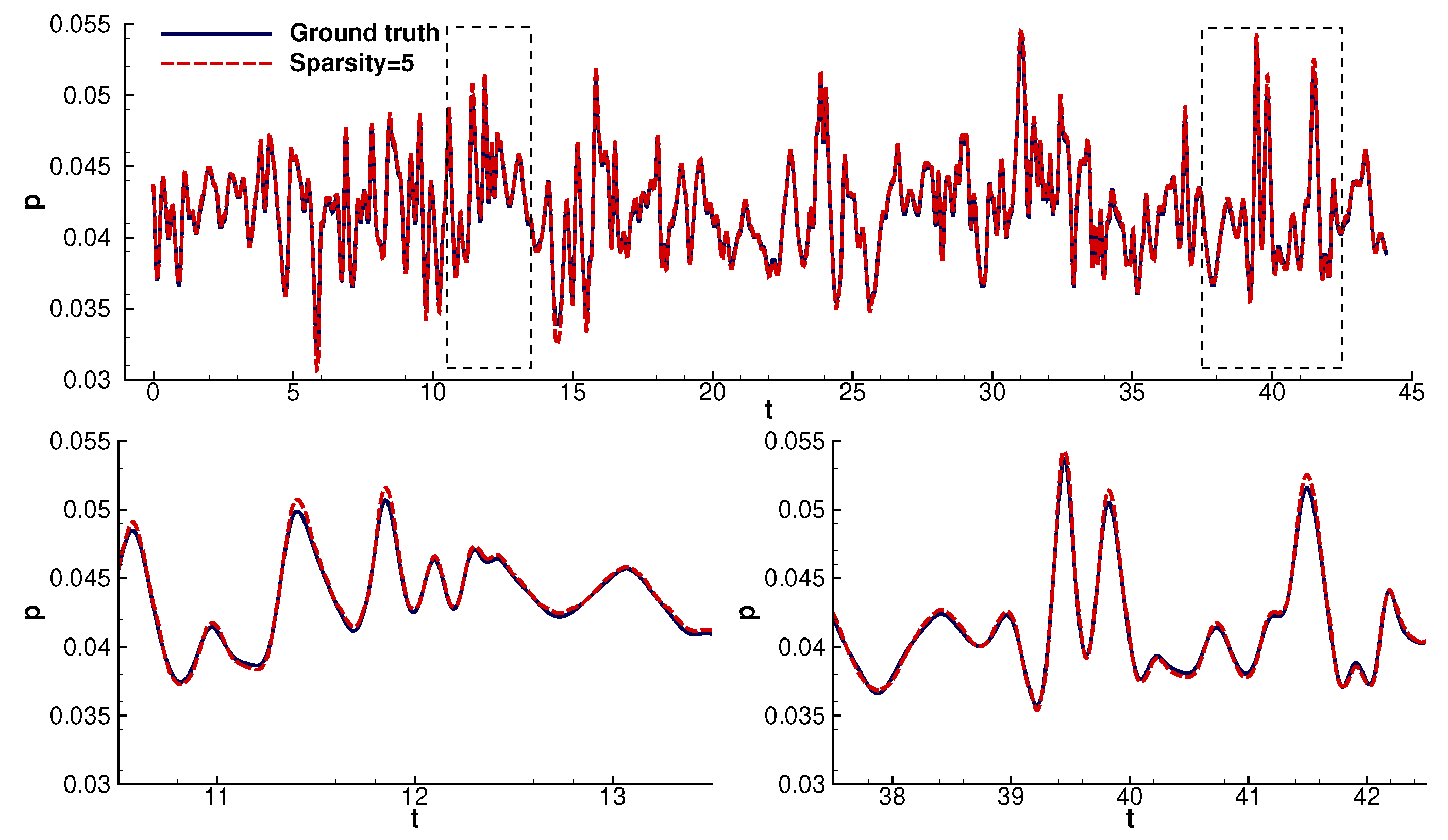
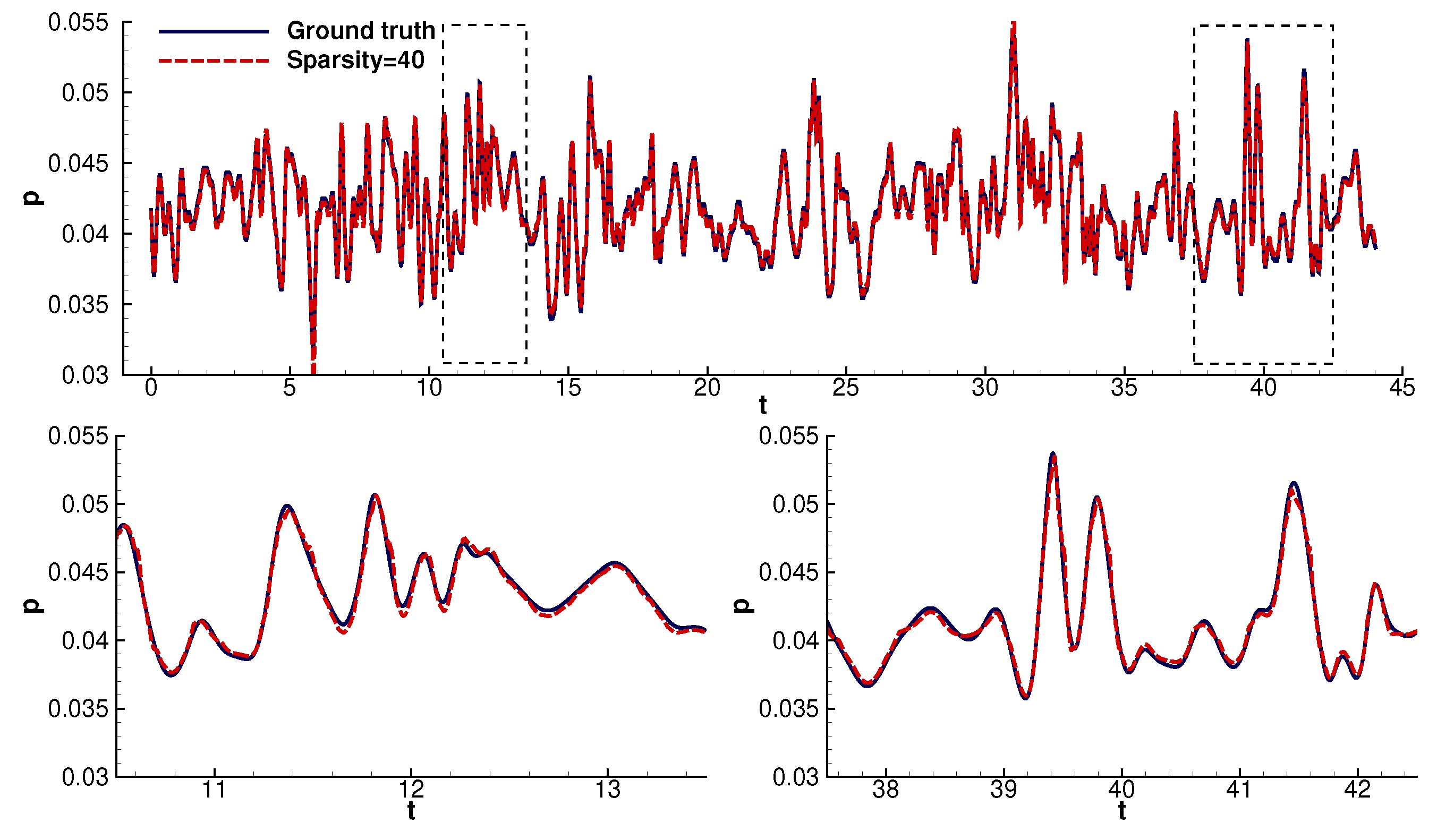
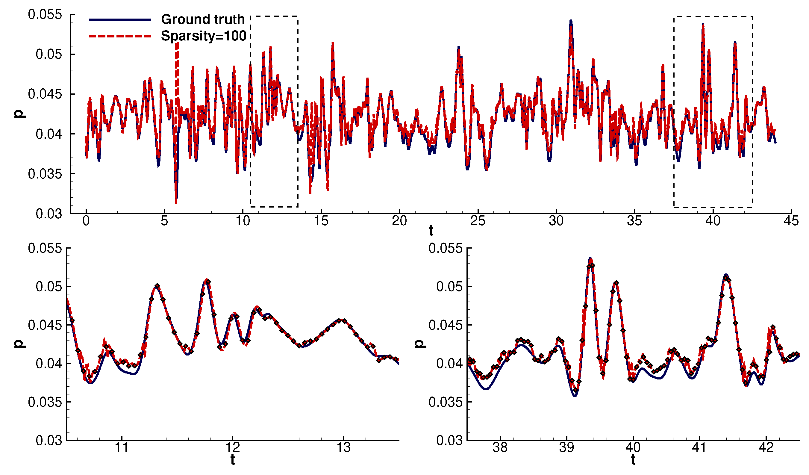
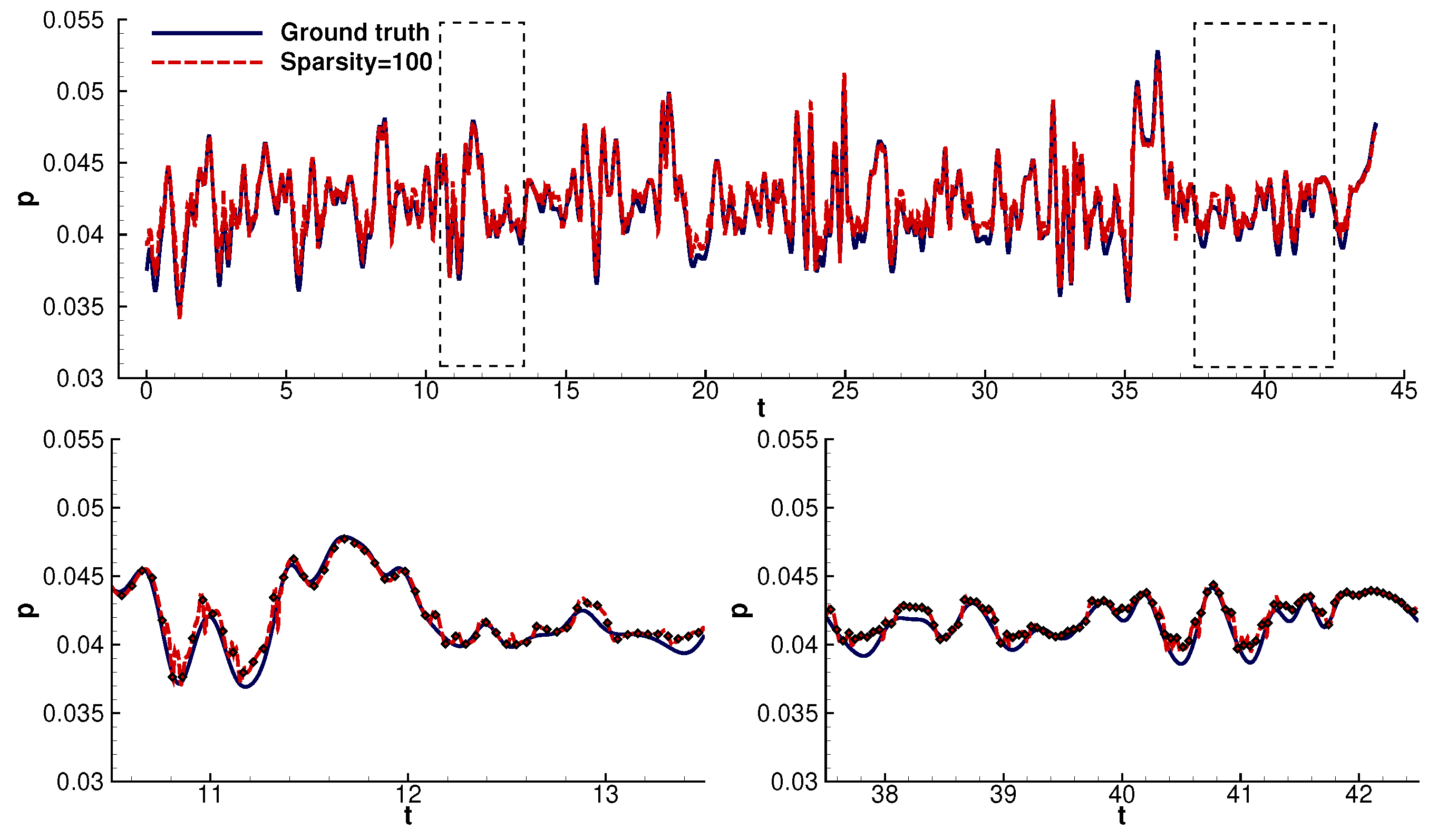
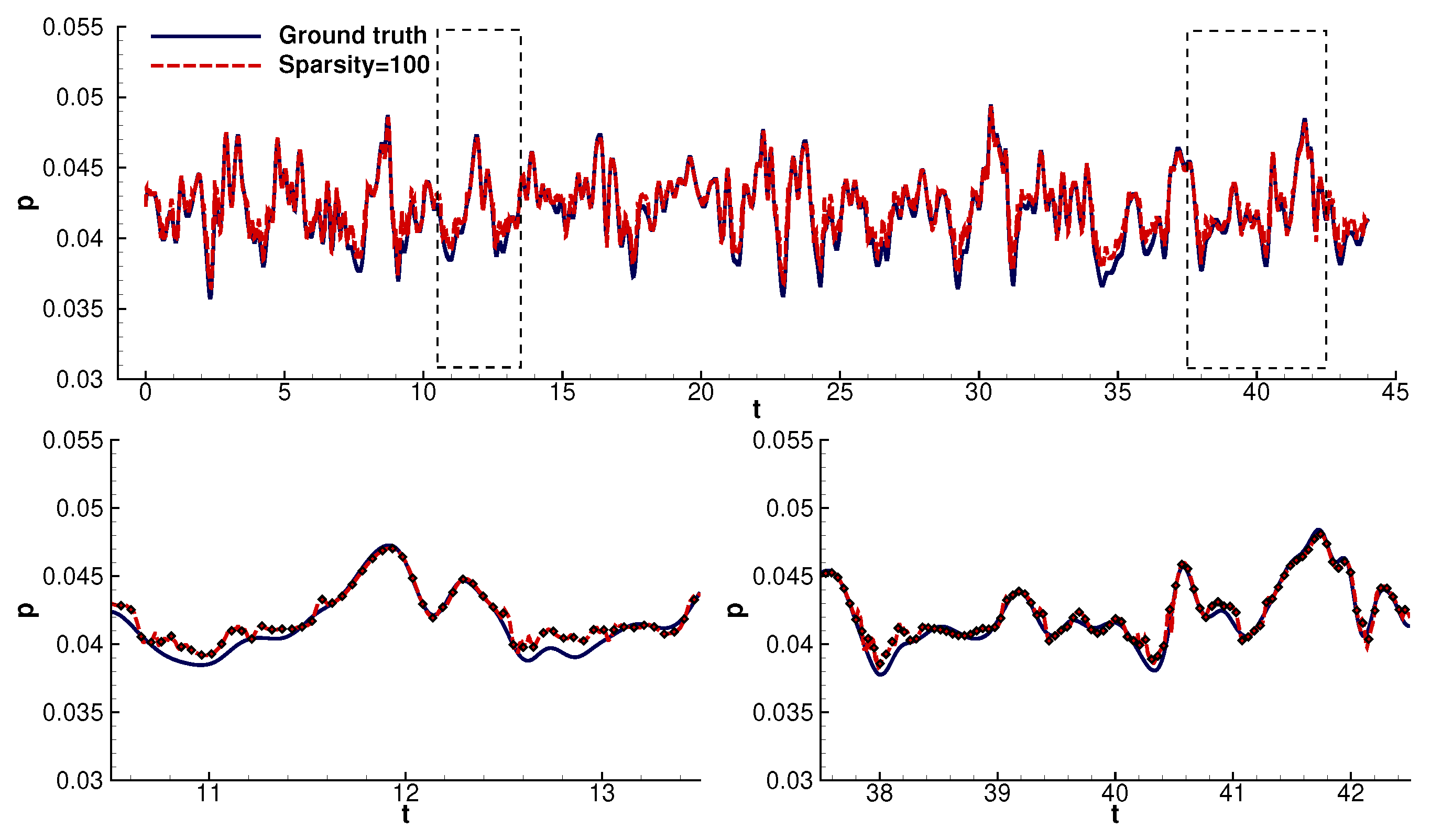
4.1. Time Domain Reconstruction

We present time domain reconstruction graphs with zoomed-in instances over randomly selected time samples. Multiple spatial points are presented for various sparsity factors covering a large part of the overall experiment’s results (Figure 4, Figure 5, Figure 6, Figure 7, Figure 8 and Figure 9).

Two important conclusions can be drawn:

• The model, initially trained on probe 2, can be transferred to unseen signals with high accuracy.
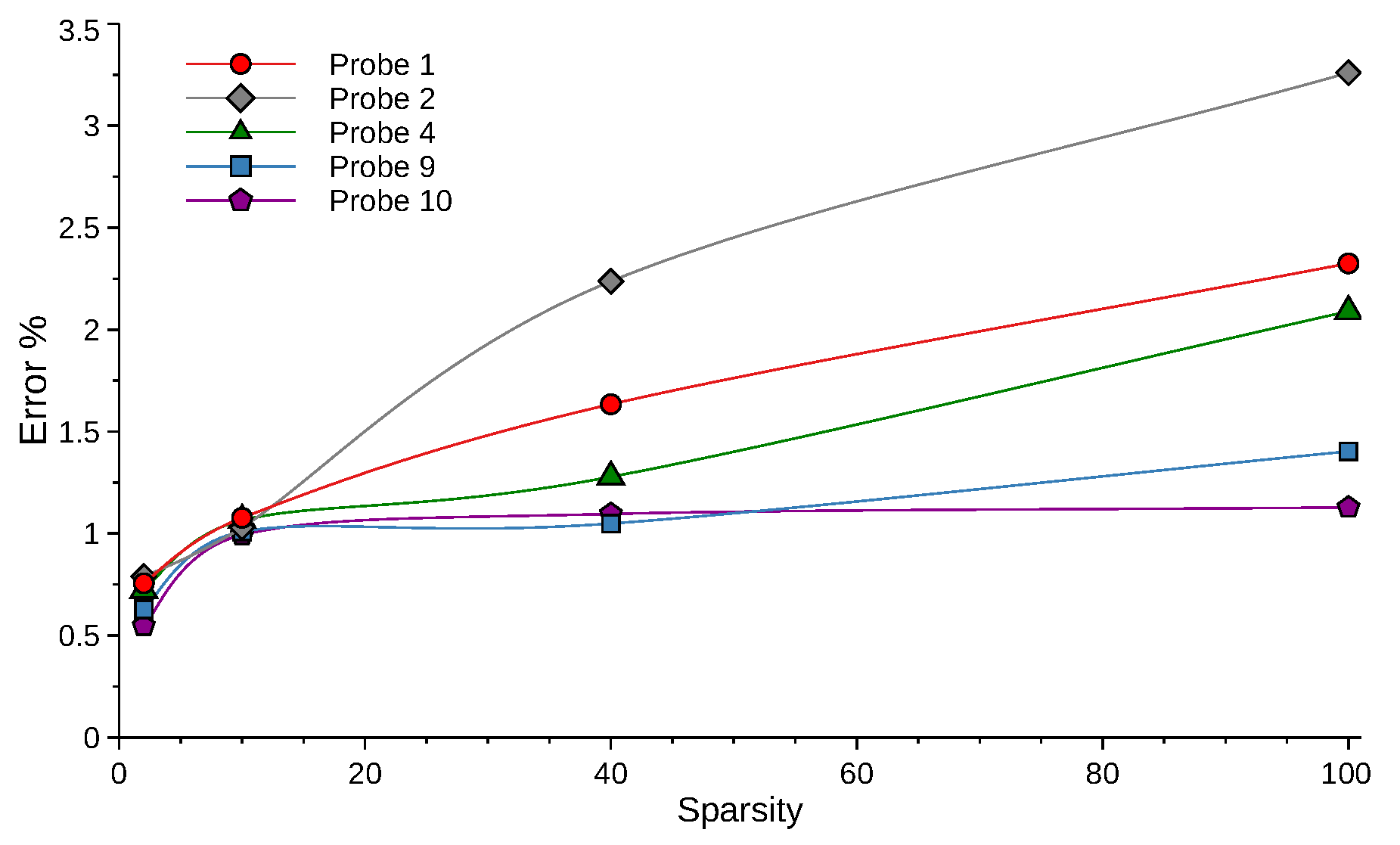
• Furthermore, the model can reconstruct the signals with less than 3% error even for an extremely high sparsity factor equal to 100. The reconstruction error remained well below 2% for sparsity factors <40 (Figure 10).

The root mean square error (RMSE) was normalized by the mean pressure signal value and given as a percentage for all sparsities (sampling steps) examined:

$$\mathrm{NRMSE}\left(p\right)\%=100\times \frac{\mathrm{RMSE}\left(p\right)}{\overline{p}}$$

(8)

where the RMSE is the square root of the mean square error (MSE):

$$\mathrm{RMSE}\left(p\right)=\sqrt{\mathrm{MSE}\left(p\right)}=\sqrt{\frac{1}{n}\sum _{i=1}^n{\left(p_i-\overline{p}\right)}^2}$$

Here, $\overline{p}$ is the mean pressure value at each probe location:

$$\overline{p}=\frac{1}{n}\sum _{i=1}^n{p}_i$$

where i indicates the index location in the temporal pressure signal (vector) of a length n. Here, the temporal probe signals comprise a total of n = 86,098 samples each.

The normalized RMSE error shows that our model outperformed the unseen signals compared with the training signal (Figure 10). Probe groups $\{1,2,3\}$ (and separate groups $\{4,5,6\}$, $\{7,8,9\}$, and $\{10,11,12\}$) belong to the same streamwise location, meaning that the signal turbulence properties should be homogeneous (as was discussed earlier in Section 2.3). Except for probes 1 and 2, the error of the other probes from the same group behaved similarly. The error at the training probe (probe 2) tended to be the highest among the other probes, though we note that the error generally remained low for all probes. This suggests that the model learned to follow a general behavior in all signals, and our training successfully avoided overfitting the model to the training signal. Moreover, the complexity of each signal may also affect its error growth with increasing sparsity. This behavior can be random due to the stochasticity of turbulent signals.

To avoid overfitting, we employed regularization (dropout), used the last 20% of the signal as a validation set, applied early stopping based on the validation loss, and employed a small batch size of 32 as discussed in Section 3. Additionally, after experimenting with various architectural hyperparameters, we chose one that provided a relatively small model, since larger models can easily overfit noise in the training data.

The normalized RMSE of reconstruction seems to followed a linear relationship up to a sparsity factor of 20. Then, the error’s rate of increase seemed to reduce, but the error variance between different probes increased. Interestingly, the reconstruction of certain probes was slightly improved when the sparsity factor was increased from 20 to 40. For the present data set and examined probes, a sparsity of 15 ($St\simeq 20$) marks the limit below which the spatially unresolved frequencies began to contaminate the temporal signal (i.e., the oscillations were created mainly due to numerical noise, as will be discussed later in Section 4.2). Hence, the sparsity value of 20 was near to the value marking the “transition” from the resolved physical oscillations to the numerical noise-contaminated region. The above might suggest that the LSTM model training was, to some extent, affected by the nonphysical numerical noise oscillations present, as implied by the error being smallest for sparsity values near 15 (or $St\approx 20$) (i.e., when the LSTM model predictions predominantly occur across the numerical noise-contaminated frequency range). This point deserves further investigation using time series filtered from the high-frequency numerical noise and cross-examined across other turbulent flow cases.

We can see that the reconstruction model could infer most values with high accuracy, partially losing precision in the areas of abrupt gradients and slightly overestimating the pressure fluctuation value (Figure 4, Figure 5, Figure 6, Figure 7, Figure 8 and Figure 9). The ability of the model to predict the areas around abrupt gradients was hindered as the sparsity increased. Even though the model could still follow the signal’s trend, we observed lagging. Even the high-sparsity models precisely followed the linear parts of the signals.

4.2. Power Spectrum Analysis

Pressure fluctuations have an essential effect on the structural response of aerospace structures, particularly at high speeds. The fundamental statistical quantity that describes the magnitude of near-wall acoustic loading is the power spectrum of pressure fluctuations. According to the theoretical arguments made by Ffowcs-Williams [45] and high-resolution numerical simulations [24,25] for compressible flows, the scaling should be $\omega \to 0$ in the low-frequency region, where $\omega =2\pi f$ is the angular frequency [24,25]. This observation has been confirmed by the experimental and numerical studies of supersonic and hypersonic turbulent boundary layers [24,46,47,48,49]. The above contradicts the Kraichnan–Phillips theorem for incompressible flows [50,51,52], which suggests ${\omega }^2$.

Importantly, it is the low-frequency pressure oscillations that had the largest power, as is evident in Figure 11. Moreover, the natural frequencies of most aero-structural components tend to be within this low-frequency domain, further exacerbating the problem. Thus, regarding the structural response to the turbulent flow pressure fluctuations, the energy-containing range of the pressure power spectrum (i.e., low frequencies) is the most critical one.

The objective here is to examine the accuracy of the LSTM predictions of the power spectra. The results for different probe positions and sparsity factors are presented in Figure 11, where the frequency (x) axis relates to the dimensionless Strouhal number as defined previously in Section 2.3$\left(St=f^{*}{\delta }_{x_{45}}/U_{\infty }\right)$.

The cut-off dimensionless frequencies (Strouhal numbers) corresponding to sparsities of 5, 40, and 100 were $St\simeq 60$, $\simeq 7.5$, and $\simeq 3$, respectively. The results in Figure 11 indicate, however, that for a sparsity equal to 5, the effect from the LSTM reconstruction began to affect the power spectrum from a much lower frequency, specifically $St\simeq 8.5$, instead of at its corresponding cut-off value of $St\simeq 60$. For short time intervals (high frequencies) relative to the intrinsic time scale of the pressure fluctuations, the LSTM interpolation predictions were poorer than those for simpler linear interpolation methods. For example, cubic spline interpolation had little to no effect until its corresponding cut-off frequency, a value which was much higher than the plotted frequency range.

The pressure fluctuations corresponding to the frequencies above $St>20$ are not shown in Figure 11 since they were above the spatially resolved turbulence scales. As an explicit time-stepping algorithm was employed (details given in Section 2.2), the numerical method’s time step size was restricted by the Courant–Friedrichs–Lewy (CFL) condition, where for the DNS [25], $\mathrm{CFL}=0.5$ was employed. At the same time, the high Mach number of the particular case ($M=6$) resulted in a sound speed of ${\lambda }_{1,3}=u\pm c$, whose amplitude was several times larger than the entropy wave (${\lambda }_2=c$). Since the flow velocity tended to zero nearer to the no-slip wall ($u\to 0$), all pressure waves eventually traveled at an equivalent acoustic speed c (i.e., at a larger time scale than the one required for the numerical stability of the simulation). Consequently, the high-frequency power spectra content comprised mostly numerical “noise” that practically had no physical meaning and was thus omitted from the graphs.

Several further observations can be drawn from the power spectra results in Figure 11. First, the lower frequencies were predicted with high accuracy, even for high sparsity. This was consistent across the locations on the panel. Second, LSTM could not reconstruct the high frequencies, with the error increasing significantly for a sparsity of 100. Third, the significant departure of the predictions from the ground truth occurred around a Strouhal number of ∼0.7 for sparsities of 5 and 40, and this was consistent across the locations. Furthermore, the results show that examining the accuracy of the time series (preceding section) did not guarantee the accuracy of the DL predictions across frequencies. The DL accuracy should be considered for the application’s objective. The model gave promising results for low-frequency oscillations relevant to acoustic fatigue. This was partly due to the capability of DL methods to utilize fine-grained data in the learning phase, which enables them to later upsample coarse-grained data. Mathematical interpolation techniques cannot achieve such a task since sparse time series signals inherently possess low wavenumber information. This, however, is particularly true for the high-frequency part of the signals. Indeed, the low wavenumber component does not need super-resolution reconstruction. In fact, for extremely large sparsities whose cut-off frequency reaches near or even into the energy-containing range of the turbulent signal power spectrum, it was previously found that the LSTM model could not correctly predict the beginning of the inertial subrange. Since the sparsity of 100 is already sufficiently large to introduce significant errors across the signal wavelengths within the inertial subrange, applying the trained LSTM model to even greater sparsities was not considered. Even predicting acoustic frequencies related to turbulence at the highest frequencies and under high sparsity conditions still requires further development.

In the present case, the overprediction of the power spectrum content at the high frequencies obtained using the LSTM model could indeed be potentially addressed by employing a filtering or convolution layer (or something similar). However, previous studies employing the LSTM model [17,18] for different sets of turbulent wall pressure signals found that the LSTM model, in contrast, underpredicted the high-frequency pressure oscillations. Hence, an a priori layer proceeding with the LSTM prediction cannot be universally appropriate across the different cases and signals. The underlying reason(s) behind this contrasting response of the LSTM model, specifically at high frequencies, is an ongoing investigation. Several ideas are currently being pursued to help elucidate the issue.

5. Conclusions

DL reconstruction of wall surface pressure fluctuations in fully developed turbulent flow at a high speed of Mach 6 over a flat panel was presented. This is an extreme flow environment containing large fluctuation amplitudes within short intervals, thus making the implementation of the LSTM model challenging.

The LSTM model was applied in conjunction with spline interpolation. This is the first time DL has been used at wall surface pressure fluctuations of such high-speed boundary layers. The conclusions drawn from the present study are summarized below:

• We found through a series of numerical experiments that imputing missing intermediate values in the sampled sparse signals via cubic spline functions is effective.
• The normalized RMSE error shows that our model outperformed unseen signals compared with the training signal. This suggests that the model learned to follow a general behavior across all signals, avoiding overfitting.
• The normalized RMSE of reconstruction increased linearly up to a sparsity factor of 20. Then, the error’s rate of reduced, but the error variance between different probes increased.
• The reconstruction model could infer most values with high accuracy. The model lost accuracy in the areas of steep gradients. The model’s departure from the ground truth increased with increasing sparsity. Despite the above, the model could still follow the signal’s trend. In particular, even at high sparsities, the model consistently followed the linear parts of the signals.
• LSTM could predict the lower frequencies of the spectrum with high accuracy, including the cases of high sparsity. The accuracy of the model was restricted in those frequencies.

Given the above results and conclusions, there are several future research directions for developing DL models for reconstructing time histories of different aerodynamic and structural dynamic parameters. Addressing the issue of the model’s accuracy in high frequencies is an area where further work needs to be carried out. Understanding DL models in flows containing shocks and shock–boundary layer interaction is interesting in high-speed flows, and work in this area is underway. Data fusion from different experiments and simulations into LSTM and the reconstruction of multivariate signals is another area of future work.

References

1. Frank, M.; Drikakis, D.; Charissis, V. Machine-Learning Methods for Computational Science and Engineering. Computation 2020, 8, 15. [Google Scholar] [CrossRef]
2. Agliari, E.; Barra, A.; Barra, O.A.; Fachechi, A.; Franceschi Vento, L.; Moretti, L. Detecting cardiac pathologies via machine learning on heart-rate variability time series and related markers. Sci. Rep. 2020, 10, 8845. [Google Scholar] [CrossRef] [PubMed]
3. Graves, A. Generating Sequences with Recurrent Neural Networks. arXiv 2014, arXiv:1308.0850. [Google Scholar] [CrossRef]
4. Yadav, A.; Jha, C.K.; Sharan, A. Optimizing LSTM for time series prediction in Indian stock market. Procedia Comput. Sci. 2020, 167, 2091–2100. [Google Scholar] [CrossRef]
5. Althelaya, K.A.; El-Alfy, E.S.M.; Mohammed, S. Evaluation of bidirectional LSTM for short-and long-term stock market prediction. In Proceedings of the 2018 9th International Conference on Information and Communication Systems (ICICS), Irbid, Jordan, 3–5 April 2018; pp. 151–156. [Google Scholar] [CrossRef]
6. Muduli, P.R.; Gunukula, R.R.; Mukherjee, A. A deep learning approach to fetal-ECG signal reconstruction. In Proceedings of the 2016 Twenty Second National Conference on Communication (NCC), New Delhi, India, 4–6 March 2016; pp. 1–6. [Google Scholar] [CrossRef]
7. Yamamoto, K.; Hiromatsu, R.; Ohtsuki, T. ECG Signal Reconstruction via Doppler Sensor by Hybrid Deep Learning Model with CNN and LSTM. IEEE Access 2020, 8, 130551–130560. [Google Scholar] [CrossRef]
8. Tong, W.; Li, L.; Zhou, X.; Hamilton, A.; Zhang, K. Deep learning PM2.5 concentrations with bidirectional LSTM RNN. Air Qual. Atmos. Health 2019, 12, 411–423. [Google Scholar] [CrossRef]
9. Nakamura, T.; Fukami, K.; Hasegawa, K.; Nabae, Y.; Fukagata, K. Convolutional neural network and long short-term memory based reduced order surrogate for minimal turbulent channel flow. Phys. Fluids 2021, 33, 25116. [Google Scholar] [CrossRef]
10. Fukami, K.; Fukagata, K.; Taira, K. Machine-learning-based spatio-temporal super resolution reconstruction of turbulent flows. J. Fluid Mech. 2021, 909, A9. [Google Scholar] [CrossRef]
11. Liu, B.; Tang, J.; Huang, H.; Lu, X.Y. Deep learning methods for super-resolution reconstruction of turbulent flows. Phys. Fluids 2020, 32, 25105. [Google Scholar] [CrossRef]
12. Chen, H.; Guo, M.; Tian, Y.; Le, J.; Zhang, H.; Zhong, F. Intelligent reconstruction of the flow field in a supersonic combustor based on deep learning. Phys. Fluids 2022, 34, 35128. [Google Scholar] [CrossRef]
13. Fukami, K.; Fukagata, K.; Taira, K. Super-resolution reconstruction of turbulent flows with machine learning. J. Fluid Mech. 2019, 870, 106–120. [Google Scholar] [CrossRef]
14. Spottswood, S.M.; Beberniss, T.J.; Eason, T.G.; Perez, R.A.; Donbar, J.M.; Ehrhardt, D.A.; Riley, Z.B. Exploring the response of a thin, flexible panel to shock-turbulent boundary-layer interactions. J. Sound Vib. 2019, 443, 74–89. [Google Scholar] [CrossRef]
15. Brouwer, K.R.; Perez, R.A.; Beberniss, T.J.; Spottswood, S.M.; Ehrhardt, D.A. Experiments on a Thin Panel Excited by Turbulent Flow and Shock/Boundary-Layer Interactions. AIAA J. 2021, 59, 2737–2752. [Google Scholar] [CrossRef]
16. Ritos, K.; Kokkinakis, I.W.; Drikakis, D. Physical insight into the accuracy of finely-resolved iLES in turbulent boundary layers. Comput. Fluids 2018, 169, 309–316. [Google Scholar] [CrossRef]
17. Poulinakis, K.; Drikakis, D.; Kokkinakis, I.W.; Spottswood, S.M. Machine-Learning Methods on Noisy and Sparse Data. Mathematics 2023, 11, 236. [Google Scholar] [CrossRef]
18. Poulinakis, K.; Drikakis, D.; Kokkinakis, I.W.; Spottswood, S.M. Deep learning reconstruction of pressure fluctuations in supersonic shock–boundary layer interaction. Phys. Fluids 2023, 35, 76117. [Google Scholar] [CrossRef]
19. Song, W.; Gao, C.; Zhao, Y.; Zhao, Y. A Time Series Data Filling Method Based on LSTM—Taking the Stem Moisture as an Example. Sensors 2020, 20, 5045. [Google Scholar] [CrossRef]
20. Mondal, D.; Percival, D. Wavelet variance analysis for gappy time series. Ann. Inst. Stat. Math. 2008, 62, 943–966. [Google Scholar] [CrossRef]
21. Karaca, Y.; Zhang, Y.; Muhammad, K. A Novel Framework of Rescaled Range Fractal Analysis and Entropy-Based Indicators: Forecasting Modelling for Stock Market Indices. Expert Syst. Appl. 2019, 144, 113098. [Google Scholar] [CrossRef]
22. Manousopoulos, P.; Drakopoulos, V.; Theoharis, T. Curve fitting by fractal interpolation. Trans. Comput. Sci. I 2008, 4750, 85–103. [Google Scholar]
23. Raubitzek, S.; Neubauer, T. A fractal interpolation approach to improve neural network predictions for difficult time series data. Expert Syst. Appl. 2021, 169, 114474. [Google Scholar] [CrossRef]
24. Ritos, K.; Drikakis, D.; Kokkinakis, I. Acoustic loading beneath hypersonic transitional and turbulent boundary layers. J. Sound Vib. 2019, 441, 50–62. [Google Scholar] [CrossRef]
25. Drikakis, D.; Ritos, K.; Spottswood, S.M.; Riley, Z.B. Flow transition to turbulence and induced acoustics at Mach 6. Phys. Fluids 2021, 33, 76112. [Google Scholar] [CrossRef]
26. Drikakis, D.; Hahn, M.; Mosedale, A.; Thornber, B. Large eddy simulation using high-resolution and high-order methods. Philos. Trans. R. Soc. A Math. Phys. Eng. Sci. 2009, 367, 2985–2997. [Google Scholar] [CrossRef] [PubMed]
27. Kokkinakis, I.; Drikakis, D. Implicit Large Eddy Simulation of weakly-compressible turbulent channel flow. Comput. Methods Appl. Mech. Eng. 2015, 287, 229–261. [Google Scholar] [CrossRef]
28. Kokkinakis, I.W.; Drikakis, D.; Ritos, K.; Spottswood, S.M. Direct numerical simulation of supersonic flow and acoustics over a compression ramp. Phys. Fluids 2020, 32, 66107. [Google Scholar] [CrossRef]
29. Balsara, D.S.; Shu, C.W. Monotonicity Preserving Weighted Essentially Non-oscillatory Schemes with Increasingly High Order of Accuracy. J. Comput. Phys. 2000, 160, 405–452. [Google Scholar] [CrossRef]
30. Toro, E.F.; Spruce, M.; Speares, W. Restoration of the contact surface in the HLL-Riemann solver. Shock Waves 1994, 4, 25–34. [Google Scholar] [CrossRef]
31. Toro, E.F. Riemann Solvers and Numerical Methods for Fluid Dynamics, A Practical Introduction, 3rd ed.; Springer: Berlin/Heidelberg, Germany, 2009. [Google Scholar] [CrossRef]
32. Spiteri, R.; Ruuth, S. A New Class of Optimal High-Order Strong-Stability-Preserving Time Discretization Methods. SIAM J. Numer. Anal. 2002, 40, 469–491. [Google Scholar] [CrossRef]
33. Yu, Y.; Si, X.; Hu, C.; Zhang, J. A review of recurrent neural networks: LSTM cells and network architectures. Neural Comput. 2019, 31, 1235–1270. [Google Scholar] [CrossRef]
34. Ullah, M.; Ullah, H.; Khan, S.D.; Cheikh, F.A. Stacked LSTM network for human activity recognition using smartphone data. In Proceedings of the 2019 8th European Workshop on Visual Information Processing (EUVIP), Roma, Italy, 28–31 October 2019; pp. 175–180. [Google Scholar]
35. Ghanbari, R.; Borna, K. Multivariate time-series prediction using LSTM neural networks. In Proceedings of the 2021 26th International Computer Conference, Computer Society of Iran (CSICC), Tehran, Iran, 3–4 March 2021; pp. 1–5. [Google Scholar]
36. Deng, Z.; Chen, Y.; Liu, Y.; Kim, K.C. Time-resolved turbulent velocity field reconstruction using a long short-term memory (LSTM)-based artificial intelligence framework. Phys. Fluids 2019, 31, 75108. [Google Scholar] [CrossRef]
37. Li, Y.; Chang, J.; Wang, Z.; Kong, C. An efficient deep learning framework to reconstruct the flow field sequences of the supersonic cascade channel. Phys. Fluids 2021, 33, 56106. [Google Scholar] [CrossRef]
38. Lin, W.C.; Tsai, C.F. Missing value imputation: A review and analysis of the literature (2006–2017). Artif. Intell. Rev. 2020, 53, 1487–1509. [Google Scholar] [CrossRef]
39. Beylkin, G. On the Fast Fourier Transform of Functions with Singularities. Appl. Comput. Harmon. Anal. 1995, 2, 363–381. [Google Scholar] [CrossRef]
40. Carbone, M.; Bragg, A.D.; Iovieno, M. Multiscale fluid–particle thermal interaction in isotropic turbulence. J. Fluid Mech. 2019, 881, 679–721. [Google Scholar] [CrossRef]
41. Kingma, D.P.; Ba, J. Adam: A Method for Stochastic Optimization. arXiv 2014, arXiv:1412.6980. [Google Scholar]
42. Kandel, I.; Castelli, M. The effect of batch size on the generalizability of the convolutional neural networks on a histopathology dataset. ICT Express 2020, 6, 312–315. [Google Scholar] [CrossRef]
43. Masters, D.; Luschi, C. Revisiting Small Batch Training for Deep Neural Networks. arXiv 2018, arXiv:1804.07612. [Google Scholar]
44. Maas, A.L. Rectifier Nonlinearities Improve Neural Network Acoustic Models. In Proceedings of the 30th International Conference on Machine Learning, Atlanta, GA, USA, 7–19 June 2013; Volume 28. [Google Scholar]
45. Ffowcs-Williams, J.E. Surface pressure fluctuations induced by boundary layer flow at finite Mach number. J. Fluid Mech. 1965, 22, 507–519. [Google Scholar] [CrossRef]
46. Beresh, S.J.; Henfling, J.F.; Spillers, R.W.; Pruett, B.O.M. Fluctuating wall pressures measured beneath a supersonic turbulent boundary layer. Phys. Fluids 2011, 23, 75110. [Google Scholar] [CrossRef]
47. Bernardini, M.; Pirozzoli, S.; Grasso, F. The wall pressure signature of transonic shock/boundary layer interaction. J. Fluid Mech. 2011, 671, 288–312. [Google Scholar] [CrossRef]
48. Duan, L.; Choudhari, M.M.; Zhang, C. Pressure fluctuations induced by a hypersonic turbulent boundary layer. J. Fluid Mech. 2016, 804, 578–607. [Google Scholar] [CrossRef]
49. Zhang, C.; Duan, L.; Choudhari, M.M. Effect of wall cooling on boundary-layer-induced pressure fluctuations at Mach 6. J. Fluid Mech. 2017, 822, 5–30. [Google Scholar] [CrossRef]
50. Phillips, O.M. On the aerodynamic surface sound from a plane turbulent boundary layer. Proc. R. Soc. A 1956, 234, 327–335. [Google Scholar] [CrossRef]
51. Bull, M.K. Wall-pressure fluctuations beneath turbulent boundary layers: Some reflections on forty years of research. J. Sound Vib. 1996, 190, 299–315. [Google Scholar] [CrossRef]
52. Kraichnan, R.H. Pressure Fluctuations in Turbulent Flow over a Flat Plate. J. Acoust. Soc. Am. 2005, 28, 378–390. [Google Scholar] [CrossRef]
Figure 1. Vorticity contour plot near the wall in the fully turbulent region. The x axis indicates the distance from the plate’s leading edge, and the y axis is the spanwise position, with both shown in reduced units (normalized by  x l ). The numbered black stars indicate the probes’ positions to calculate the pressure fluctuations induced by the flow on the wall.
Computation 12 00004 g001
Figure 2. Illustration of pressure fluctuation for probe 2 in the time domain: (top) original signal, (middle) sparsity = 40, and (bottom) sparsity = 100. All values are dimensionless.
Computation 12 00004 g002
Figure 3. High-level schematic of the neural network architecture. The length of the sequence L is dynamic and depends on the sampling step  = m s p a r s i t y _ f a c t o r . The symbols  h t  and  c t  denote the LSTM cell’s hidden state and cell state outputs, respectively. The model’s inputs and output are  X t  and  X L + 1 , respectively.
Computation 12 00004 g003
Figure 4. Predictions of the hybrid LSTM model at probe 1 for a sparsity factor equal to 5. We zoomed in on random samples to better visualize and evaluate the reconstruction error.
Computation 12 00004 g004
Figure 5. Predictions of the hybrid LSTM model at probe 1 for a sparsity factor equal to 40. We zoomed in on random samples to better visualize and evaluate the reconstruction error.
Computation 12 00004 g005
Figure 6. Predictions of the hybrid LSTM model at probe 1 for a sparsity factor equal to 100. We zoomed in on random samples to better visualize and evaluate the reconstruction error.
Computation 12 00004 g006
Figure 7. Predictions of the hybrid LSTM model at probe 4 for a sparsity factor equal to 100. We zoomed in on random samples to better visualize and evaluate the reconstruction error.
Computation 12 00004 g007
Figure 8. Predictions of the hybrid LSTM model at probe 9 for a sparsity factor equal to 100. We zoomed in on random samples to better visualize and evaluate the reconstruction error.
Computation 12 00004 g008
Figure 9. Predictions of the hybrid LSTM model at probe 10 for a sparsity factor equal to 100. We zoomed in on random samples to better visualize and evaluate the reconstruction error.
Computation 12 00004 g009
Figure 10. Normalized RMSE % vs. the sparsity factor used to sample the training dataset.
Computation 12 00004 g010
Figure 11. Power spectrum of the original signal (ground truth) and the LSTM prediction for different sparsities at probes (from top to bottom and left to right) 1, 2 (training point), 4, 9, and 10. The x axis is the Strouhal number, and the y axis is the power spectrum in terms of pascals squared.
Computation 12 00004 g011