A Deep Learning Approach for Brain Tumor Firmness Detection Based on Five Different YOLO Versions: YOLOv3–YOLOv7

Abstract

Brain tumor diagnosis traditionally relies on the manual examination of magnetic resonance images (MRIs), a process that is prone to human error and is also time consuming. Recent advancements leverage machine learning models to categorize tumors, such as distinguishing between “malignant” and “benign” classes. This study focuses on the supervised machine learning task of classifying “firm” and “soft” meningiomas, critical for determining optimal brain tumor treatment. The research aims to enhance meningioma firmness detection using state-of-the-art deep learning architectures. The study employs a YOLO architecture adapted for meningioma classification (Firm vs. Soft). This YOLO-based model serves as a machine learning component within a proposed CAD system. To improve model generalization and combat overfitting, transfer learning and data augmentation techniques are explored. Intra-model analysis is conducted for each of the five YOLO versions, optimizing parameters such as the optimizer, batch size, and learning rate based on sensitivity and training time. YOLOv3, YOLOv4, and YOLOv7 demonstrate exceptional sensitivity, reaching 100%. Comparative analysis against state-of-the-art models highlights their superiority. YOLOv7, utilizing the SGD optimizer, a batch size of 64, and a learning rate of 0.01, achieves outstanding overall performance with metrics including mean average precision (99.96%), precision (98.50%), specificity (97.95%), balanced accuracy (98.97%), and F1-score (99.24%). This research showcases the effectiveness of YOLO architectures in meningioma firmness detection, with YOLOv7 emerging as the optimal model. The study’s findings underscore the significance of model selection and parameter optimization for achieving high sensitivity and robust overall performance in brain tumor classification.

1. Introduction

Cancer remains a global challenge, with millions of lives lost annually. Brain tumor diagnosis, particularly meningioma firmness detection, presents complexities and uncertainties in manual magnetic resonance imaging (MRI) analysis. Existing processes, subject to human variation, are time consuming and may lack accuracy. To bridge this gap, this study proposes a You Only Look Once YOLO-based approach for automated meningioma firmness classification, addressing the need for precise and efficient brain tumor diagnosis. The research problem revolves around optimizing the performance of meningioma firmness detection by leveraging cutting-edge deep learning architectures, specifically the YOLO model. Objectives include adapting YOLO for meningioma classification, evaluating variants, and optimizing parameters for sensitivity and training time. This study aims to contribute to the medical and computing communities by enhancing tumor detection and classification accuracy. This introduction establishes the context, underscores the significance of automated tumor detection, and introduces YOLO as a promising solution.

In 2020 alone, there were approximately 19.3 million new cancer cases and nearly 10.0 million cancer-related deaths worldwide, highlighting the urgency for advanced diagnostic methods [1,2]. Conventional MRI tumor detection lacks consistency, prompting the demand for automated systems coupling machine learning with image processing. Meningioma tumors vary from soft to firm, necessitating distinct treatments. The proposed YOLO model aligns with the growing trend of utilizing machine learning (ML) and deep learning (DL) for medical applications, offering potential improvements in efficiency and accuracy. The subsequent sections delve into the methodology, results, and conclusions, detailing this study’s contribution to both the medical and computational realms.

Brain tumors, with diverse categories such as gliomas, medulloblastoma, and meningioma, underscore the need for accurate and swift detection [3]. Among these, glioblastoma and meningioma present distinct challenges, with the latter exhibiting a spectrum from soft to firm consistency. It is a tumor that grows from the membranes that surround the brain and spinal cord (meninges). Most of the meningiomas are noncancerous. In this regard, the presence of soft meningioma requires tissue suction, while finding a firm one necessitates surgery by opening the skull to eradicate the tumor. Thus, the prescription of an appropriate treatment in order to preserve the chances of a patient’s survival requires the identification and classification of brain tumors into a soft or firm category using an effective and accurate detection system.

Current medical imaging techniques, notably magnetic resonance imaging (MRI), play a pivotal role in identifying brain tumors [3]. However, challenges persist in precise and swift classification. The proposed YOLO-based approach aims to overcome these challenges by offering a real-time object detection system with the potential for enhanced sensitivity and accuracy. Magnetic resonance imaging (MRI) is an advanced medical scan that utilizes radio waves and powerful magnetic fields to create detailed images of the body’s organs and tissues. Its versatility allows examination of various body parts, including the brain, bones, and heart, making it effective for detecting diverse diseases. MRI plays a crucial role in identifying areas of injury, particularly by visualizing water, a key component of the human body. A water molecule is made up of two hydrogen atoms and one oxygen atom (denoted as H₂O). This method relies on the alignment and manipulation of hydrogen nuclei (protons) through powerful magnets and radio frequency, ultimately producing images based on the protons’ behavior in a magnetic field. The resulting signals, generated during a process called precession, are measured and translated into meaningful images [3]. 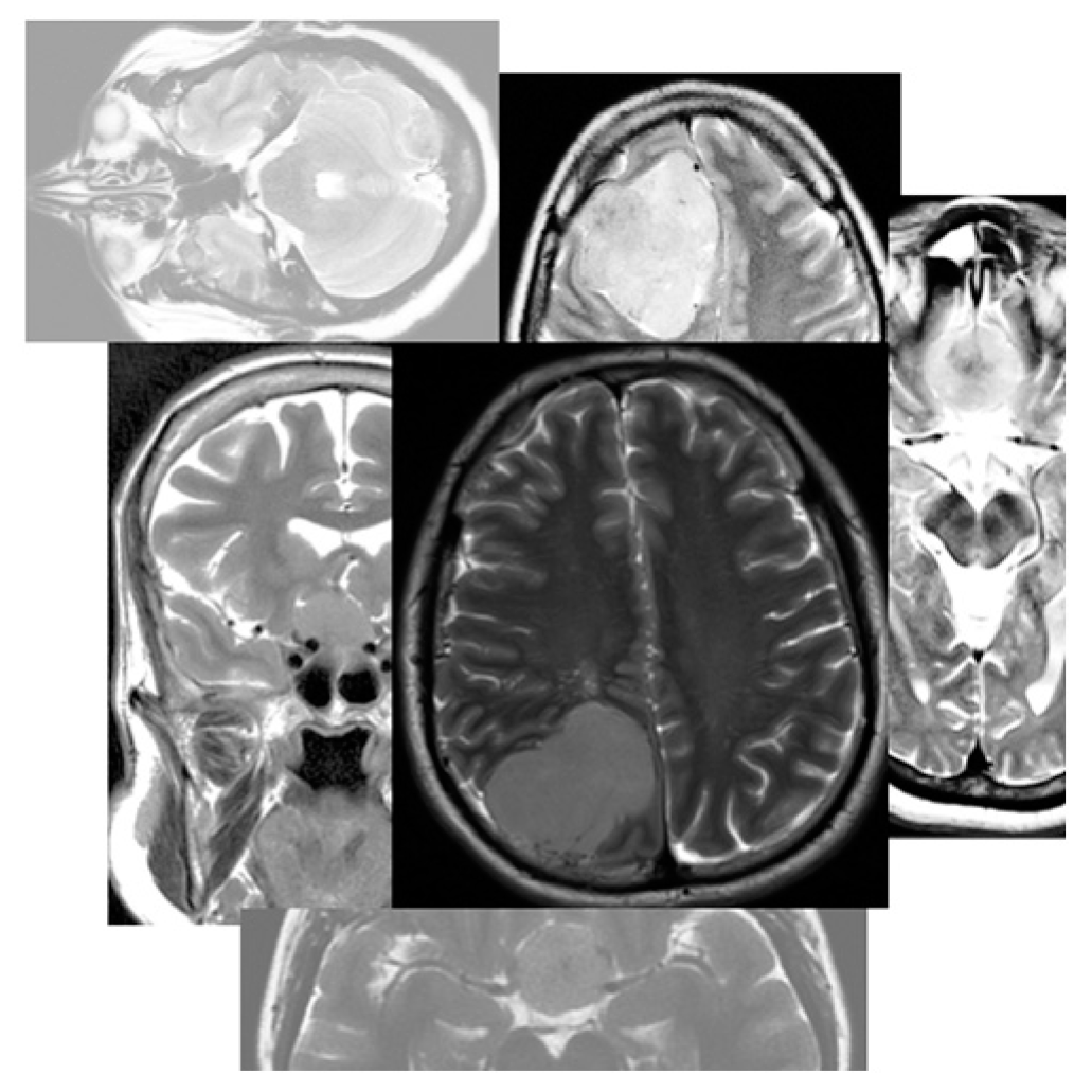Figure 1 shows a real meningioma classification process with clear labels from the KKUH dataset.

This study also explores the broader landscape of ML and DL in medical applications, particularly in computer-aided diagnosis (CAD). ML techniques aid in feature extraction, and DL, with its ability to discern patterns without explicit programming, proves advantageous. The proposed YOLO system aligns with the paradigm shift toward deep learning, demonstrating its potential for meningioma firmness classification. The utilized technique splits the input image into a grid of cells, and each cell directly predicts the coordinates of a bounding box, where the large number of candidate bounding boxes are consolidated into a final class probability prediction for these bounding boxes. The subsequent sections detail the experimental setup, results, and comparisons, providing insights into the model’s performance.

In conclusion, this research addresses the limitations of current meningioma firmness detection methods through a YOLO-based approach. By combining advancements in deep learning with medical imaging, this study contributes to the fields of both medicine and computing. The subsequent sections elucidate the methodology, showcase experimental results, and draw conclusions on the efficacy of the proposed YOLO model in enhancing meningioma detection accuracy. Here is a brief explanation of the several metrics used in evaluating the performance of a model. Specificity corresponds to the ability to correctly identify patients who have a soft tumor as being negative [4]. The mAP is a metric used to evaluate the accuracy of object detection models, while the F1-score is defined as the harmonic mean of precision and recall. It is used as a statistical measure to rate classification performance across the entire dataset. Balanced accuracy serves as a comprehensive measure of a model’s performance, taking into account both sensitivity and specificity. This metric is especially valuable in handling imbalanced datasets, as it calculates the average of sensitivity and specificity with equal weighting. A high level of balanced accuracy reflects an effective balance between correctly predicting positives and negatives. Precision assesses the accuracy of positive predictions, representing the ratio of correctly predicted positive observations to the total predicted positives. A higher precision signals a lower occurrence of false positives.

The rest of this paper is organized as follows: Section 2 presents some of the literature review for the detection of brain tumors using both shallow learning models and deep learning models. In Section 3, we describe the methodology we used for detecting the firmness of meningioma tumors. We experiment and discuss our results of using YOLO versions and compare them with some of the other recent performance results in Section 4 before we conclude the paper.

2. Literature Review

Due to the scarcity of related research that addresses the tumor firmness detection problem, we outline relevant machine learning methods that have been considered for detecting brain tumors using magnetic resonance images (MRIs). In particular, this section summarizes the relevant state-of-the-art contributions over the last 15 years. Broadly speaking, shallow machine learning models require the extraction of relevant low-level features, which consists of a manual process that involves a thorough data domain knowledge. In other words, such shallow-model-based solutions rely on learning using predefined features extracted from the considered data collection [5].

The authors in [5] proposed a clustering algorithm based on particle swarm optimization (PSO) to find the centroids of a number of clusters that enclose together brain tumor patterns obtained from MRI images. The solution introduced in [6] extracts discrete wavelet transform (DWT) from input images as the feature extraction step. Then, the dimensionality of the resulting feature vectors is reduced using principal component analysis (PCA). To decide whether the image is normal or abnormal, forward back-propagation artificial neural network (FP-ANN) or k-nearest neighbor (k-NN) classifiers are used leading to different accuracy results. In [7], feature extraction has been implemented using MATLAB 7.9.0 (R2009B) to classify the input MRI brain images into normal and abnormal by using support vector machine (SVM). The input data are mapped into a higher dimensional space using a radiant basis function (RBF) kernel.

The researchers in [8] proposed a methodology for a CAD Brain MRI system. Specifically, a feedback pulse-coupled neural network (FPCNN) is used for the segmentation and the detection of the region of interest (ROI), while DWT is employed for feature extraction. One should note that PCA is also used for dimensionality reduction. In addition, a backpropagation NN is used for classifying whether the image is normal or abnormal. In [9], after applying generalized autoregressive conditional heteroscedasticity (GARCH), the authors used PCA and linear discriminant analysis (LDA) to remove the redundancy and extract the proper features. Then, to determine the tumor in a given MRI image, they employed KNN and SVM classifiers. The work outlined in [10] relies mainly on a genetic algorithm (GA), curve fitting, and support vector machine. In particular, GA was used to extract segments from the images. Further, in order to properly segment the images without the loss of information and improve the procedure of segmentation, the authors also used curve fitting. The resulting features are then classified using SVM. The methodology introduced in [11] consists of a set of stages starting from an MRI image input. The image is then processed through the enhancement of MRI images, skull stripping, fuzzy c-means, and feature extraction. Finally, the SVM classifier shows if the brain image has a tumor or not.

The method in [12] used histogram fast segmentation-self organizing map (HFS-SOM) clustering and texture feature extraction via a gray-level co-occurrence matrix (GLCM). Moreover, principal component analysis (PCA) was used for feature selection followed by proximal support vector machine (PSVM) to classify the image into normal, benign, or malignant tumors. Similarly, the authors in [13] employed PCA to reduce the number of features and fed the resulting features into two well-known algorithms: neural network (NN) and support vector machine (SVM) for classification of human brain MRIs. In [14], the authors investigated histogram-based features, shape descriptors, and fuzzy local binary pattern (fLBP) features as well as multiresolution texture features to encode the image visual properties. Moreover, they employed a random forest (RF) technique to classify the extracted features into different brain tumor types. One should also mention that rough entropy thresholding was deployed for feature quantification prior to the RF-based classification task.

In [15], the researchers developed an adaptive neuro-fuzzy classifier based on linguistic hedges (ANFC-LH) to select the significant features and predict the tumor grade. Namely, they extracted gray-level statistic (GLS), gray-level co-occurrence matrix (GLCM), geometrical shape and size (GSS), and gray-level run length (GLRL) features from the collection of MRI images. The accuracy achieved using ANFC-LH was 85.83%. Similarly, in [16], GLCM features were extracted from MRI images after a preprocessing phase including noise removal and a median filter-based image enhancement task. Afterwards, a genetic algorithm was applied as a metaheuristic optimization to predict the tumor categories. In [17], the authors used a k-means clustering based segmentation technique to extract the region of interest from a given image. Then, the discrete wavelet transform (DWT) was used to extract the texture feature from the resulting regions. Next, the PCA algorithm was deployed to reduce the features’ dimensionality. Finally, the obtained features were conveyed into a support vector machine (SVM) algorithm in order to map them into the predefined brain tumor categories. This classification approach yielded an accuracy of 99%. In [18], a deep-learning-based feature extraction was coupled with the handcrafted descriptor, modified gray-level co-occurrence matrix (MGLCM), to improve the accuracy of the SVM-based classification task using MRI brain scans. The reported accuracy attained 99.30%.

A hybrid feature extraction method was introduced by the authors of [19]. Initially, the brain images were transformed into intensity images as a preprocessing step. Then, the images’ visual properties were encoded using the PCA-based normalized GIST (PCA-NGIST) hybrid method. Finally, brain tumors were detected using the robust layered ensemble model (RLEM) classifier. This hybrid method’s accuracy reached 94.23%. Recently, the work described in [4] aimed at recognizing meningioma tumor cases using a computer-aided diagnosis (CAD) system that relies on a supervised machine learning technique. Particularly, the authors investigated different feature extraction techniques and concluded that the local binary pattern descriptor exhibits a considerable discrimination capability that allows for an accurate detection of meningioma tumor firmness.

The authors in [20] proposed an extended Kalman filter with support vector machine (EKF-SVM)-based method. Their algorithm has five components, including standardizing all images. Afterwards, noise is removed with a nonlocal means filter, and contrast is enhanced with improved dynamic histogram equalization. For feature extraction, a gray-level co-occurrence matrix is used. In the third step, the extracted features are fed into an SVM to classify the MRI initially, and an EKF is used to classify brain tumors in the MRIs. The accuracy of the classifier is verified using cross-validation. Finally, a combination of k-means clustering and region growth is used for detecting brain tumors as an automatic segmentation method. They achieved 96.05% accuracy. The authors of [21] focused on a multiclass support vector machine (M-SVM) classifier to identify the meningioma, glioma, and pituitary tumors from the brain tumor dataset. Their proposed method has five steps. First, the edges in the image were determined by linear contrast stretching. Second, the segmentation of brain tumors was developed by a custom 17-layered deep neural network (DNN). Third, they used modified MobileNetV2 architecture for feature extraction. Fourth, they used an entropy-based controlled method, where the best features are selected based on the entropy value. The final features are classified using an M-SVM classifier. The obtained results for the accuracy, sensitivity, and specificity were 97.47%, 97.22%, and 97.94% respectively. In [22], the authors conducted their experiment on a collected database from Aarthi Hospital, to detect glioma tumors into benign tumors and malignant tumors, where the results they obtained were 100% for sensitivity, 97.2% for accuracy, and 90% for specificity. Their proposed work is divided into three parts: preprocessing segmentation and classification steps are applied on brain MRI images, texture features are extracted using gray-level co-occurrence matrix (GLCM), DWT, and then classification is achieved using SVM.

Based on the papers reviewed above, one can deduce that the most frequent classification techniques used by researchers are SVM and CNN. These two classifiers were used in eighteen papers and in nine papers, respectively. Another observation is that KNN was used in four of the referenced works, while the rest of the classifiers were used less often. One can also notice that CNN was used nine times, whereas RNN was only used once in the last 15 years. On the other hand, the most used feature extraction methods are GLCM and DWT. They were exploited in ten papers and seven papers, respectively, while PCA, LBP, and GLRL were used about twice a time. The remaining feature extraction techniques were employed about once. In addition, one can observe that over the last 15 years the methods that were considered the most for tumor detection are supervised learning and deep learning techniques. On the other hand, hybrid methods were used less frequently in the detection of tumors. As it can be noticed, despite the considerable efforts made to tackle brain tumor detection using machine learning techniques, only a few contributions have been introduced to address the meningioma firmness detection problem. Moreover, and to the best of our knowledge, the use of state-of-the-art pre-trained deep learning models has not been employed before to classify meningioma cases into firm or soft classes.

3. Proposed Approach

The purpose of this research is to advance the detection of meningioma firmness utilizing a YOLO (You Only Look Once)-based methodology, seeking an optimal balance between detection speed and accuracy for assessing meningioma firmness.

The system’s workflow, as depicted in Figure 2, begins with the employment of a YOLO model pretrained on the expansive COCO dataset. The weight parameters of this model were trained with the COCO 20-class dataset. Leveraging this pretrained model affords us a foundational weight parameter set, primed with a broad understanding of visual features. Through the technique of transfer learning, we adapt this model to concentrate on two classes of our specific classification task and differentiate between two types of meningioma firmness. The rationale behind adopting transfer learning lies in its ability to expedite the learning process, enhance accuracy, and reduce the need for extensive training data. Transfer learning involves leveraging knowledge acquired from learning a related task, resulting in improved efficiency when applied to a new but related task. To further enhance the model’s generalization and robustness, data augmentation techniques were applied during the training phase. These techniques involve artificially expanding the training dataset by applying random transformations to the input images, such as rotations, flips, and changes in brightness. By exposing the model to a variety of augmented images, the risk of overfitting to the original dataset is mitigated, contributing to better generalization when presented with new and unseen data.

The model’s output encompasses the coordinates of the bounding box, the class name of each object (representing the tumor type), and a confidence score. If the predicted bounding boxes deviate significantly from the labeled bounding boxes, the system fails to detect the object accurately. This combined approach of transfer learning and data augmentation serves the purpose of preventing overfitting and overtraining issues commonly associated with deep learning networks when confronted with limited datasets. The following details annotate the YOLO architecture specifically for meningioma classification:

• Input Layer Adjustments: Given that MRI images differ from the common objects in the COCO dataset, the input layer is tuned to accommodate the unique grayscale intensity distributions of MRI scans.
• Hyperparameter Optimization: The hyperparameters, including the learning rate, batch size, and number of epochs, are calibrated specifically for the task, ensuring the model learns effectively from the MRI data without overfitting.
• Custom Loss Function: The loss function is tailored to emphasize the precision of bounding box localization and class prediction accuracy.
• Evaluation Metrics: The model’s performance is assessed using metrics such as intersection over union (IoU) for bounding box accuracy and F1 scores for classification, reflecting the model’s efficacy in meningioma detection and firmness differentiation.
• Postprocessing Thresholds: Custom thresholds for confidence scores and nonmaximum suppression are established to refine the detection output, minimizing false positives and false negatives.

This meticulous customization of the YOLO architecture to the domain of MRI analysis for meningioma classification is anticipated to yield a model that not only performs with high accuracy but also operates at a speed conducive to clinical application. This approach demonstrates a promising pathway to integrate deep learning models in medical imaging diagnostics, providing valuable support to radiologists and enhancing the overall quality of patient care.

Our system divides the input image into an S × S grid. If the center of an object falls into a grid cell, that grid cell is accountable for detecting that object. The images are only looked at once to predict objects of interest and their respective locations. In particular, the algorithm relies on a single convolutional network whereby the prediction of multiple bounding boxes and class probabilities are simultaneously performed. It is noted that the training of YOLO is conducted using full images. In other words, no prior segmentation is required by the utilized approach. As illustrated in Figure 3, YOLO’s main goal aims at dividing the input image into many grid cells. Each grid cell is responsible for predicting the object centered in that grid cell, the bounding boxes, and the confidence scores for the corresponding detected boxes. The cells predict the class probabilities, which are used to establish the class of each object. The intersection over union (IoU) measure ensures that the predicted bounding boxes are equal to the real boxes of the objects. This removes unnecessary bounding boxes that do not meet the characteristics of the objects. The final detection consists of unique bounding boxes that fit the objects perfectly. The predicted bounding box has its (x, y) coordinates, in terms of height and width, and class labels as outputs, where (IoU) describes the relationship between two boundaries which are the predicted boundary vs. ground-truth boundary box. A higher IoU implies a closer match between the anticipated and actual bounding box coordinates, which gives better prediction accuracy. To train an object detection model, usually, there are two inputs, which are an image and ground-truth bounding boxes for each object in the image. IoU Equation (1) divides intersection area by union area, where a higher IoU correlates with better prediction.

(1)

The YOLO framework has three main components. They are represented by the backbone, neck, and head. The backbone part mainly extracts the essential features of an image and feeds them to the head through the neck. The neck collects feature maps extracted by the backbone and creates feature pyramids. Finally, the head consists of output layers that have the final detections. Each version of YOLO introduces something new in terms of its characteristics and internal structure to improve its performance.

3.1. YOLO Framework

In addition to the backbone, neck, and head components, YOLO also uses input images as shown in Figure 4. During the training step, the data augmentation approach is applied to the input to diversify the training data. In other words, the purpose of data augmentation is to increase the variability of the input images. This would enhance the generalization capability of the model. Specifically, photometric and geometric distortion are considered to augment the data. In fact, the photometric distortion is intended to change the brightness, contrast, saturation, and noise of the MRI image, while the geometric distortion includes random scaling, cropping, flipping, and rotating MRIs, as illustrated in Figure 5. The resulting diversified instances are then conveyed to the backbone for feature extraction through the different network levels. The backbone mainly determines the feature extractor representation ability. Meanwhile, its design has a critical influence on the inference efficiency since it carries a large portion of the computational cost.

The neck provides feature infusion using upsampling and feature concatenation layers to add more details for the last part, which are used to aggregate the low-level physical features with high-level semantic features and then build up pyramid feature maps at all levels to fusion different stage feature maps. Moreover, the head provides the final predictions to the classes as well as the bounding boxes of detected objects with the confidence. Next, we proceed to describe each of the five versions of the YOLO deep learning model starting with YOLOv3.

The adaptation of the YOLO architecture for meningioma classification involved several key modifications. The grid system was customized for precise tumor localization, opting for a full-image training approach due to the complex nature of meningioma tumors. Integration of the intersection over union (IoU) measure during training ensured a closer match between predicted and actual bounding box coordinates. Framework components, including the backbone, neck, and head, were enhanced to focus on meningioma characteristics. The performance measures have been updated in each YOLO version to match our needs in detecting meningioma firmness. These modifications aimed at refining detection accuracy and overall model performance in meningioma classification within medical imaging.

3.2. YOLOv3

For YOLOv3, a Darknet53 library [23,24] is typically used as the backbone to extract relevant features from the input images. As explained above, the backbone is composed of convolution layers whose function is to extract essential features from the input images. On the other hand, a feature pyramid network (FPN) [25] forms the neck, which plays an important role in extracting the feature maps from different stages. Finally, the head role consists mainly in performing the final prediction and generating a vector containing bounding box coordinates: width, height, class label, and class probability.

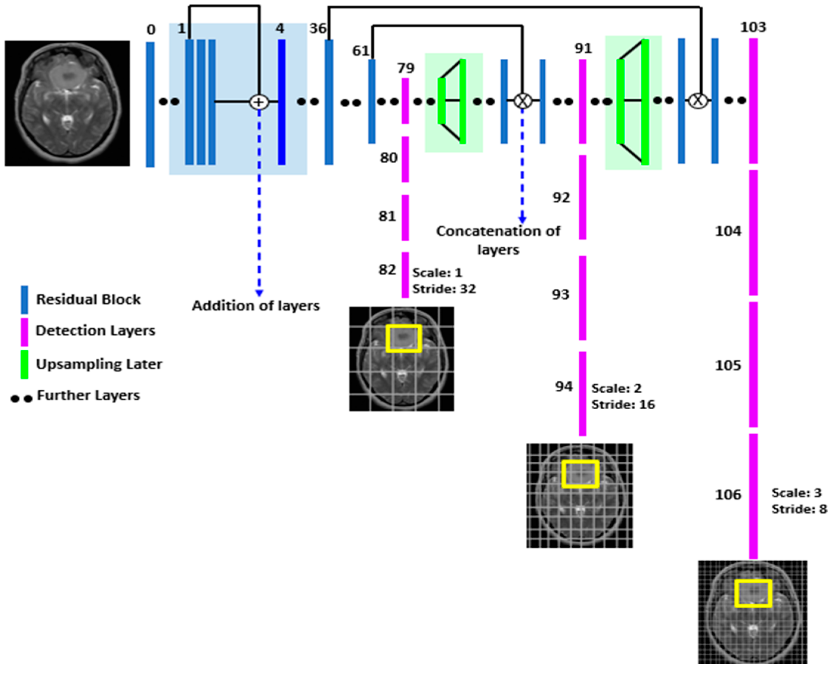
Accordingly, after an image is fed into Darknet53 for feature extraction, it is conveyed to the feature pyramid network for feature fusion. The classification results are then identified. What differentiates this YOLO version from the previous one is its ability to make detections at three different scales. It also has 106 convolutional layers and 1024 filters in Darknet53. The architecture of YOLOv3 is depicted in Figure 6. In fact, the first YOLO version, known as YOLOv1, predicts a single object per grid cell. This makes the built model simpler, but it creates issues when a single cell has more than one object. The next version succeeding it, that is YOLOv2, allows for the prediction of five bounding boxes from a single cell, while the backbone for YOLOv2 is DarkNet-19 containing a total of 19 convolutional layers. YOLOv3 overcomes the limitations of YOLOv2 and YOLOv1 by detecting features at three different scales, especially in the detection of smaller objects [25].

3.3. YOLOv4

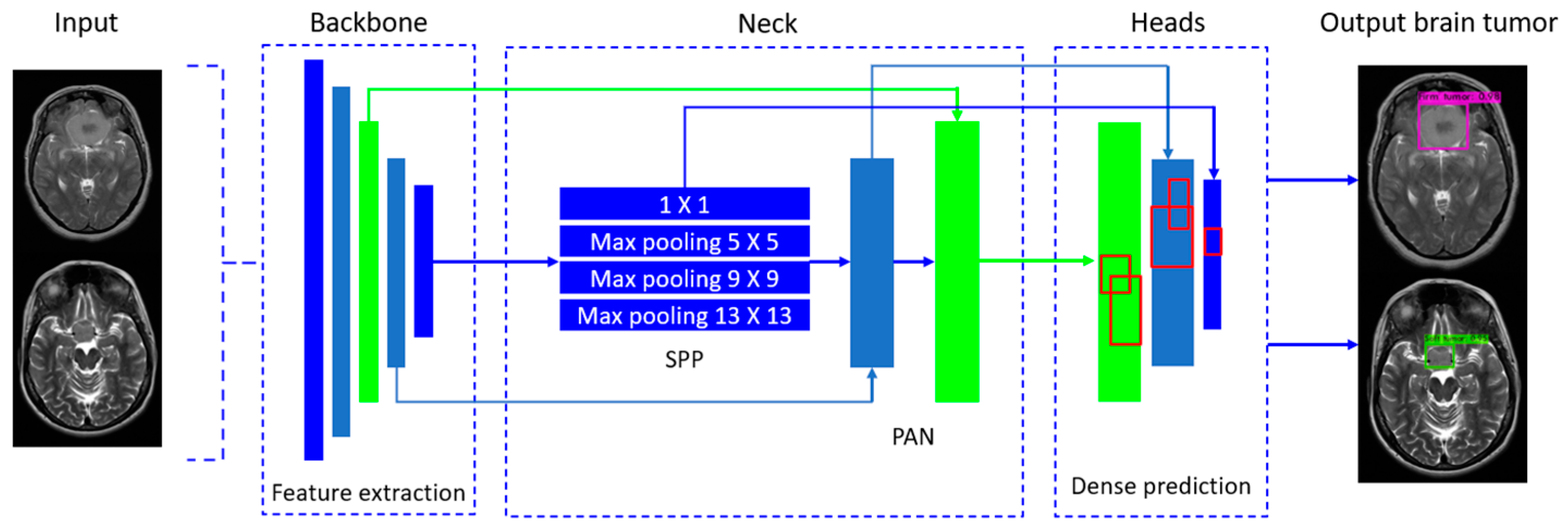
YOLOv4 exhibits advantages over other object detection methods such as deformable parts models (DPMs) and region-based convolutional neural networks (R-CNNs) [27]. As depicted in Figure 7, YOLOv4 relies on three main components [28]: the backbone, then the neck, and finally the dense prediction as the head part. The backbone deals with feature extraction and is handled by a pretrained model called CSPDarknet53. The latter divides the current layer into two parts: one that passes through the convolution layer and another that does not. This is followed by the aggregation of these results. The backbone encloses five residual block modules, and the output feature maps are connected to the neck component of YOLOv4. The neck part adds layers between the backbone and the dense prediction (head), where the neck contains a spatial pyramid pooling (SPP) module and a path aggregation network (PAN). The SPP module in the neck combines the max-pooling outputs of the low-resolution feature map to identify the most representative features. The SPP module uses kernels of size 1-by-1, 5-by-5, 9-by-9, and 13-by-13 for the max-pooling operation. The stride value is set to 1. Then, it fuses them with the high-resolution feature maps by using a PAN, which combines the low-level and high-level features by using upsampling and downsampling operations to set bottom-up and top-down paths. One should note that PAN uses the feature maps collected for predictions. Furthermore, the neck connects the feature maps from each layer of the backbone network and sends them as inputs to the head. After the collected features are processed, the head determines the bounding boxes, abjectness scores, and classification scores. The YOLOv4 network uses one-stage object detectors, such as those of YOLOv3 [28,29].

3.4. YOLOv5

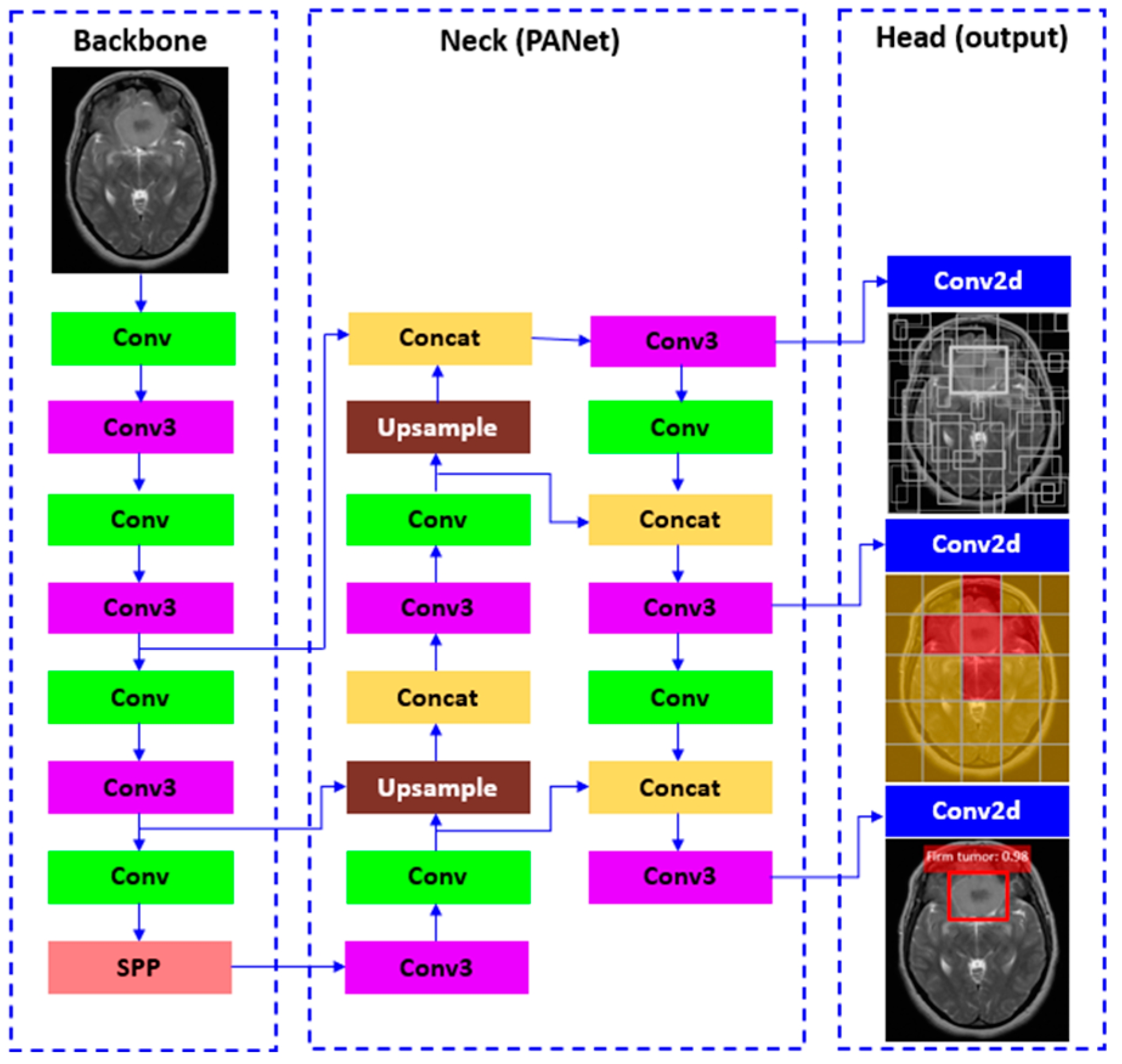
YOLOv5 was developed by Ultralytics and uses CSPDark-net53 as the backbone. This eliminates in large backbones the repetitive gradient information and integrates gradient change into the feature map that decreases the inference speed, increases accuracy, and decreases the model size by reducing the parameters. In particular, the model utilizes path aggregation network (PANet) as the neck to raise the information flow, which enhances the localization in lower layers and improves the localization accuracy of the object. PANet uses a new frame proposal network (FPN) which includes multiple bottom-up and top-down layers to enhance the propagation of low-level features in the model. The head generates three different outputs of feature maps to realize multiscale prediction as with YOLOv4 and YOLOv3, thus enhancing the prediction. The architecture of this model is shown in Figure 8. As it can be seen, Conv represents a convolution layer, while Conv3 encloses three convolution layers and a module cascaded by various bottlenecks. On the other hand, SPP is a pooling layer that is used to remove the fixed size constraint of the network. In addition, the Upsample module is used to upsample the previous layer fusion in the nearest node, while Concat is a slicing layer that is used to slice the previous layer. Finally, the last three Conv2d are detection modules used in the head. The output image is entered into CSPDarknet53 for feature extraction and then passed to PANet for feature fusion. Ultimately, the bounding box, object class, and confidence score results are obtained by the head [20,31]. The use of a focus structure with CSPdarknet53 as backbone represents the main difference between YOLOv5 and the previous YOLO versions. In particular, YOLOv4 uses CSPdarknet53 only as its corresponding backbone. The advantage of using a focus layer in YOLOv5 is the reduced requirement of CUDA memory, reduced number of layers (single layer instead of three layers in YOLOv3), and increased forward propagation and backpropagation [32].

3.5. YOLOv6

YOLOv6 was developed by a Chinese company (Meituan, Inc., Beijing, China) and was officially published in September of 2022. The backbone, denoted as EfficientRep, is used for small models. The main component of the backbone is RepBlock, used during the training phase. Each RepBlock is converted to stacks of 3 × 3 convolutional layers (denoted as RepConv). However, for medium and large model networks, the backbone is called the CSPStackRep Block. The neck of YOLOv6 is identified as Rep-PAN. To build an efficient decoupled head, the hybrid-channel strategy was used by reducing the number of the middle 3 × 3 convolutional layers to only one. The width of the head is jointly scaled by the width multiplier for the backbone and the neck. These modifications further reduce computational costs to achieve a lower inference latency [33]. Within the brain, the classification and detection branches do not share the parameters and branch out from the backbone independently. This increases accuracy while also reducing the number of computations needed. The main differences from the previous model are that YOLOv6 uses EfficientRep, RepBlock, and RepConv as a backbone, whereas YOLOv5 uses a focus structure with Cross Stage Partial DarkNet 53 (CSPdarknet53), Figure 9 shows the architecture of YOLOv6.

3.6. YOLOv7

The official YOLOv7 was published in July of 2022. It was shown that it surpasses all previous object detection models and YOLO versions in both speed and accuracy. In particular, it is the fastest and most accurate real-time detector when using video and surveillance cameras in the range from 5 frames per second (FPS) to 160 FPS [34].

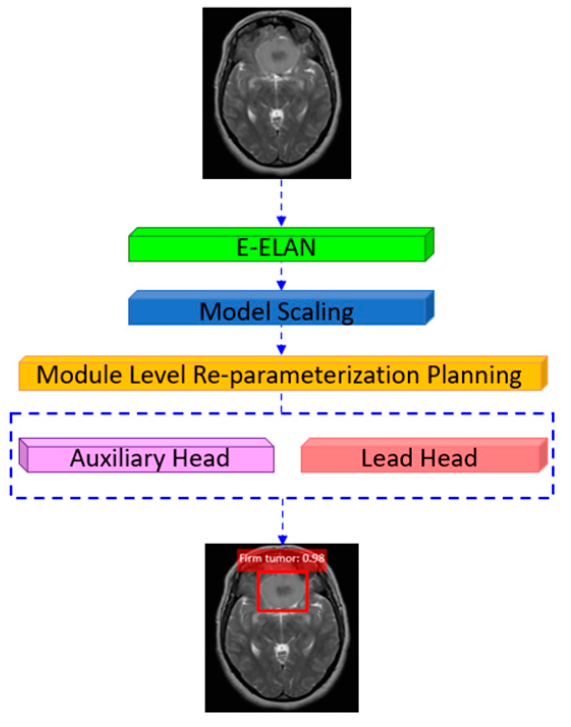
The architecture in Figure 10 of YOLOv7 presents the backbone of YOLOv7, named E-ELAN, which stands for extended efficient layer aggregation network. The YOLOv7 model’s E-ELAN architecture allows it to learn more effectively by utilizing expand, shuffle, and merge cardinality to continuously enhance the network’s capacity for learning without erasing the original gradient path. For the YOLOv7 architecture, the model scaling is improved with a compound model scaling mechanism and by the coherent scaling of the width and depth parameters for concatenation-based models. YOLOv7 uses multiple heads, where the head responsible for the final output is called the lead head. Further, the head used to assist the training process in the middle layers is called the auxiliary head. YOLOv7 has introduced the bag of freebies (BoF) methods that increase the performance of a model without increasing training cost by the use of re-parameterization, which is a technique used after training to improve the model. Even though this approach increases the training time, it improves the inference results to produce a final model that is robust in performance. There are two types of re-parametrizations used to finalize models. These are called model-level and module-level ensembles [34,35].

3.7. Discussion

The main differences between YOLOv3, YOLOv4, YOLOv5, YOLOv6, and YOLOv7 are presented in

Table 1. Comparison between the structure of YOLOv3, YOLOv4, YOLOv5, YOLOv6, and YOLOv7 deep learning models.

Model Parts	YOLOv3	YOLOv4	YOLOv5	YOLOv6	YOLOv7
Backbone	Darknet-53	CSPDarknet53 (CSPNet in Darknet)	CSPDarknet53 Focus structure	RepBlock	E-ELAN
Neck	FPN	SPP and PANet	PANet	Rep-PAN
Head	(Output layer) Bounding box Class score Confidence	(Output layer) Bounding box Class score Confidence	(Output layer) Bounding box Class score Confidence	Hybrid-channel strategy	Auxiliary head Lead head

. As it can be seen, YOLOv3 uses Darknet53 as its backbone while the YOLOv4, YOLOv5, YOLOv6, and YOLOv7 models use CSPdarknet53, focus structure with CSPDarknet53, RepBlock for small models and CSPStackRep Block for large models, and E-ELAN as their respective backbone structures. In YOLOv3, the neck plays a crucial role by extracting feature maps from various stages and using the feature pyramid network (FPN); in YOLOv4, feature aggregation is accomplished through the use of the SPP layer and PANet path aggregation, which enhances the receptive field and shorts out significant features from the backbone. The neck in YOLOv5 uses PANet and adopts a new feature pyramid network (FPN), but the YOLOv6 neck is denoted as Rep-PAN. The role of the head in one stage detector is to perform the final prediction which generates three different outputs of feature maps to achieve a multiscale prediction. It also helps to enhance the prediction of small to large objects efficiently in the model. Each successive version of YOLO is an improvement over the previous one in terms of both speed and accuracy.

4. Experiments

In this section, we have implemented and assessed the performance of the proposed YOLO-based DL approaches using a real collection of MRI images. As will be described next, a set of standard performance measures have been used to evaluate the achieved meningioma firmness detection across five different versions of the YOLO deep learning models: YOLOv3, YOLOv4, YOLOv5, YOLOv6, and YOLOv7.

4.1. Dataset Description and Preprocessing

The research experiments utilized a genuine dataset of brain tumor images generously provided by King Khalid University Hospital (KKUH) in Riyadh, Saudi Arabia [4]. This dataset comprises 28 cases involving both female and male subjects diagnosed with meningioma tumors. Out of these cases, 19 are identified as having firm tumors, while the remaining cases exhibit soft tumors. The dataset was meticulously labeled by a skilled surgeon, who leveraged their diagnostic expertise to categorize each case as either firm or soft. In total, the collected dataset encompasses 500 MRI images, which were subsequently partitioned into a training set (70% of images) and a testing set (30% of images). The training set, containing 350 MRI images, demonstrates a class distribution of 32% for soft meningioma and 68% for firm meningioma. Similarly, the testing set comprises 150 MRI images, with 32% representing soft meningioma tumors and the remaining 68% corresponding to firm cases. The two defined classes are as follows: soft tumor (class 1) and firm tumor (class 0). All images in the dataset are accompanied by .txt file labels, and the image-labeling process utilized the labelImg tool. Each object within an image is labeled in the following format:

<object-class> <x_center> <y_center> <width> <height>

The image-cropping procedure was executed manually by a qualified radiologist. This process is initiated by selecting a region of interest (ROI) covering the entire area of the brain tumor from the MRI images. The radiologist drew a rectangle box around the largest tumor area, which varied in size across cases. Subsequently, the tumor type was classified by the radiologist, as illustrated in Figure 11. This manual cropping step aimed to facilitate the training of all employed YOLO models. The experiments were conducted on Google Colaboratory, also known as “Colab”. It is an online tool by Google Corporation utilized for data analysis, machine learning, and education. The hardware accelerator employed was a NVIDIA Tesla T4 GPU, which is manufactured by NVIDIA Corporation. NVIDIA’s headquarters are located in Santa Clara, California, United States. with 40 cores, a clock rate of 1.59 GHz, and a random-access memory (RAM) of 16 GB [36].

4.2. Experimental Setup and Evaluation Metrics

The confusion matrix shown in

Table 2. Confusion matrix parameters.

Predicted	Actual
		Firm (0)	Soft (1)
	Firm (0)	TP	FP
	Soft (1)	FN	TN

represents the positive class as the firm tumor while the negative class represents the soft tumor where the term (TP) stands for True Positive. It signifies the number of correctly classified positive samples. For example, the number of frames containing a tumor is correctly estimated as having a tumor. The term True Negative (TN) denotes the number of correctly classified negative samples, that is, the number of frames not containing a tumor is correctly predicted as not having a tumor.

The False Positive (FP) term describes the number of samples incorrectly classified as positive. In other words, the number of frames not containing a tumor is incorrectly predicted as having a tumor. For the False Negative (FN) term, it signifies the number of samples classified incorrectly as negative, that is, the number of frames containing a tumor is incorrectly predicted as not having a tumor.

In order to evaluate the performance of the different YOLO-based approaches, we consider standard performance measures adopted by relevant state-of-the-art works [37]. Namely, these metrics are sensitivity (also known as recall), specificity (or selectivity), mean average precision (mAP), balanced accuracy, F1-score, and precision (also known as positive predictive value or PPV). They are presented in Equations (2) to (9) below. Further, the average precision (AP) for a given class i out of N classes is indicated by AP_i. Average precision AP is the area under the precision–recall curve. Precision and recall are always between 0 and 1. Therefore, AP falls within 0 and 1 also. Before calculating AP for the object detection, we often smooth out the zigzag pattern first as in Figure 12 by interpolating the precision at various recall levels in order to reduce the effect of the wiggles in the curve and obtain better results [38,39]. The interpolated precision P_interp at a certain recall level r is defined as the highest precision found for any recall level r′ ≥ r_(k+1) as in (6). In simple terms, it is the maximum precision value to the right, where the maximum precision corresponds to the recall value greater than the current recall value. Graphically, at each recall level, we replace each precision value with the maximum precision value to the right of that recall level. In Figure 12, the orange line is transformed into the green lines, and the curve will decrease monotonically instead of with a zigzag pattern.

The calculated AP value will be less suspectable to small variations in the ranking. Mathematically, we replace the precision value for the recall with the maximum precision for any recall [38,39]. After removing the zigzags, we measure the precise area under the precision–recall curve at each unique recall value (r₁, r₂, …). We sample p(rᵢ) whenever it drops, and we compute AP as the sum of the rectangular blocks, shown in Figure 13. This is calculated at IoU threshold 0.5 [38,39].

The sensitivity and the specificity are measures of a test’s ability to correctly classify a patient as having a disease or not. The sensitivity refers to a test’s ability to correctly identify an individual with a firm tumor as being positive. On the other hand, the specificity corresponds to the ability to correctly identify patients who have a soft tumor as being negative [4]. The mAP is a metric used to evaluate the accuracy of object detection models, while the F1-score is expressed as the precision and recall harmonic mean. It is used as a statistical measure to rate classification performance across the entire dataset. The loss rate measures how bad the model’s prediction was on a single example. If the model’s prediction is perfect, the loss is zero; otherwise, the loss is higher. Thus, the goal of training a model is to obtain a set of weights that have a low loss [40].

$$Sensitivity=\frac{TP}{TP+FN}$$

(2)

$$Specificity=\frac{TN}{TN+FP}$$

(3)

$$mAP=\frac{1}{N}{\sum }_{i=1}^{N}APi$$

(4)

$$AP=\sum \left[r_{k+1}-r_k\right]\ast P_{interp}\left(r_{k+1}\right)$$

(5)

$$P_{interp}\left(r_{k+1}\right)={\max P\left(r^{\prime }\right)}_{ r^{\prime }\ge r_{k+1}}$$

(6)

$$Balanced Accuracy=\frac{Specificity+Sensitivity}{2}$$

(7)

$$Precision=\frac{TP}{TP+FP}$$

(8)

$$F1-score=\frac{2\times (Recall\times Precision)}{Precision+Recall}$$

(9)

In this study, our intra-model analysis, the selection of optimizers, batch sizes, and learning rates were guided by the aim of optimizing model performance, particularly in terms of accuracy and training speed. We assessed two widely used optimizers, Adam and stochastic gradient descent (SGD), both known for their effectiveness in machine learning applications. The choice of optimizer is crucial, as it directly influences the model’s accuracy and training efficiency. The optimizer is a mathematical function that modifies the attributes of the neural network and is used for training a machine learning model to minimize its error rate by updating its weights. Therefore, it helps to reduce the overall loss and improve accuracy. A good optimizer is mainly focused on being faster and more efficient while showing less overfitting compared to the other for the task at hand [41,42].

Adam, an adaptive optimization algorithm, was chosen for its suitability for training deep neural networks with limited memory requirements. It computes adaptive learning rates for different parameters based on estimates of the first and second moments of gradients. Its simplicity and appropriateness for nonstationary objectives made it a compelling choice for our study [43,44].

SGD is a variant of the gradient descent method. Instead of performing computations on the whole dataset, which is redundant and inefficient, SGD only utilizes a small subset or random selection of data examples. SGD produces the same performance as regular gradient descent when the learning rate is low. It tries to update the model’s parameters more frequently, where the model parameters are changed after the computation of loss on each training example. SGD is a good optimizer when we have a lot of data and a large number of parameters. This is due to the fact that, at each step, SGD calculates an estimate of the gradient from only a random subset of that data, called a mini-batch. This is unlike gradient descent, which considers the entire dataset at each step. The advantages of SGD include the frequent updating of parameters, resulting in fast convergence while requiring less memory as there is no need to store the values of the loss functions. However, its disadvantages are its high variance in model parameters and the need to slowly reduce the value of the learning rate in order to achieve the same convergence as gradient descent [44,45].

The objective of our initial analysis was to determine the optimal optimizer (SGD or Adam) for each YOLO version. Subsequently, we conducted experiments involving varying batch sizes and learning rates. These hyperparameters play a critical role in managing the learning process and improving the resulting machine learning model’s performance. The employed hyperparameters in our various experiments are shown in

Table 3. Hyperparameters used to train and test all five YOLO versions in the detection of meningioma firmness.

Hyperparameter	Value
Batch Size	16, 32, 64
Subdivisions	16
Learning Rate	0.0005, 0.001, 0.01, 0.1
Momentum	0.949
Decay	0.0005

. The batch size is a term used in machine learning to refer to the number of training examples utilized in one iteration. It is sometimes divided by the number of subdivisions to obtain the mini-batch size, which in turn determines the number of images and samples that would fit into the RAM memory of the computing platform.

In this work, batch sizes of 16, 32, and 64, as well as 16 subdivisions, are used. It follows that the mini-batch size is equal to 64/16 = 4, 32/16 = 2, and 16/16 = 1, respectively. Such a value reflects the number of samples to be processed in one iteration, where the number of iterations is the number of batches needed to complete one epoch. An epoch is the number of times the algorithm runs on the whole training dataset. In addition, the learning rate is a hyperparameter that controls how much to change the model in response to the estimated error each time the model’s weights are updated. Further, momentum and decay are widely used parameters for gradient-based optimizers to speed up learning. They are used to control the total contribution of a gradient to future updates.

Our goal in adjusting these hyperparameters was to strike a balance between model convergence and resource efficiency. The selected hyperparameter values, as outlined in Table 3, were carefully chosen based on their impact on sensitivity and training time. The experimentation process involved systematic exploration to uncover the most effective combination, contributing to the overall optimization of the YOLO-based model for meningioma firmness detection. To enhance understanding of the model-tuning process and its impact on performance, convergence, and the decision making behind choosing optimizers, batch sizes, and learning rates for each version of YOLO involves careful considerations of model complexity, dataset characteristics, and computational resources. Popular choices like SGD and Adam have been selected based on factors such as convergence speed and memory requirements. Batch sizes of 16, 32, and 64 have been chosen based on memory constraints and training efficiency. Learning rates of 0.1, 0.01, 0.001, and 0.0005 have been adjusted to balance convergence speed and stability. Experimentation and transfer learning considerations further inform hyperparameter selection.

4.3. Performance Results

4.3.1. Impact of Varying the Optimizer

We began our experiments by running each YOLO version with the two different optimizers, SGD and Adam, where the values used in this selection for the batch size and the learning rate are 64 and 0.01, respectively. The training results and times to achieve optimal outcomes over 400 epochs are summarized in

Table 4. Training results when using the two optimizers, Adam and SGD, with five performance measures for each YOLO version.

Performance Measure	YOLOv3		YOLOv4		YOLOv5		YOLOv6		YOLOv7
	SGD	Adam	SGD	Adam	SGD	Adam	SGD	Adam	SGD	Adam
mAP	99.50%	99.50%	92.41%	100%	99.50%	99.50%	99.50%	99.33%	100%	99.60%
Precision (PPV)	100%	100%	66.03%	100%	100%	100%	99.50%	99.30%	100%	100%
Sensitivity (Recall)	100%	100%	60.12%	99.32%	100%	100%	95.80%	94.10%	100%	99.60%
Specificity (Selectivity)	96.55%	96.33%	82.87%	100%	100%	100%	100%	99.10%	100%	86.15%
Balanced Accuracy	98.27%	98.16%	71.49%	99.66%	100%	100%	97.90%	96.60%	100%	92.87%
F1-score	100%	100%	60.67%	99.66%	100%	100%	97.61%	96.63%	100%	100%
Training time	1 h 8 min	1 h 15 min	58 min	1 h 23 min	53 min	55 min	46 min	51 min	1 h 33 min	1 h 50 min

, while

Table 5. Testing results when using the two optimizers, Adam and SGD, with five performance measures for each YOLO version.

Performance Measure	YOLOv3		YOLOv4		YOLOv5		YOLOv6		YOLOv7
	SGD	Adam	SGD	Adam	SGD	Adam	SGD	Adam	SGD	Adam
mAP	99.50%	90.80%	64.40%	99.95%	99.00%	87.00%	98.59%	88.95%	99.96%	89.00%
Precision (PPV)	98.20%	89.80%	59.00%	98.07%	94.40%	74.00%	98.60%	89.00%	98.50%	88.10%
Sensitivity (Recall)	100%	85.50%	90.40%	100%	98.00%	82.50%	92.40%	83.60%	100%	84.70%
Specificity (Selectivity)	78.68%	54.54%	78.25%	95.83%	83.33%	69.09%	94.00%	54.00%	97.95%	61.53%
Balanced Accuracy	89.34%	70.02%	84.33%	97.92%	89.90%	75.80%	91.15%	69.00%	98.97%	73.11%
F1-score	99.00%	87.00%	71.40%	99.03%	95.00%	79.00%	93.16%	86.21%	99.24%	86.00%

The bold values are the best results obtained for each YOLO version.

presents the testing results. Notably, SGD consistently outperforms Adam in testing results across all YOLO versions, except for YOLOv4, which exhibits better performance with Adam, particularly in terms of mAP, precision, sensitivity, specificity, balanced accuracy, and F1-score.

To complete the subsequent experiments, we selected the best-performing optimizer for each YOLO version based on the testing results. Sensitivity, representing the percentage of correctly predicted positive cases with firm tumors among all actual positive cases, was considered the most crucial metric in this context. This metric guided our choice of the most suitable optimizer or the optimal hyperparameter value for further consideration.

4.3.2. Impact of Varying the Batch Size

After selecting the best optimizer for each YOLO version from the previous set of experiments, we conducted additional experiments with different batch sizes of 16, 32, and 64. This comparison across the three batch sizes helps determine the most effective batch size for subsequent experiments. The corresponding training and testing results are summarized in

Table 6. Training results for three batch sizes obtained by adopting SGD in all YOLO versions, except for YOLOv4.

Performance Measure	YOLOv3, SGD			YOLOv4, Adam			YOLOv5, SGD			YOLOv6, SGD			YOLOv7, SGD
	Batch Size			Batch Size			Batch Size			Batch Size			Batch Size
	16	32	64	16	32	64	16	32	64	16	32	64	16	32	64
mAP	99.50%	99.50%	99.50%	99.12%	99.25%	100%	99.50%	99.50%	99.50%	99.48%	99.50%	99.50%	99.60%	99.60%	100%
Precision (PPV)	100%	100%	100%	97.89%	98.19%	100%	100%	99.90%	100%	99.50%	99.50%	99.50%	100%	100%	100%
Sensitivity (Recall)	100%	100%	100%	98%	98.87%	99.32%	100%	100%	100%	95.40%	95.30%	95.80%	100%	100%	100%
Specificity (Selectivity)	89.60%	91.80%	96.55%	90.63%	98.94%	100%	100%	100%	100%	100%	100%	100%	99.11%	99.11%	100%
Balanced Accuracy	94.80%	95.90%	98.27%	94.32%	98.91%	99.66%	100%	100%	100%	97.70%	97.65%	97.90%	99.55%	99.55%	100%
F1-score	100%	100%	100%	97.94%	98.52%	99.66%	100%	100%	100%	97.40%	97.35%	97.61%	100%	100%	100%
Training Time	32 min	31 min	30 min	44 min	39 min	38 min	27 min	28 min	26 min	28 min	25 min	23 min	50 min	50 min	40 min

The bold values are the best results obtained for each YOLO version.

and

Table 7. Testing results for three batch sizes obtained by applying SGD in all YOLO versions, except for YOLOv4.

Performance Measure	YOLOv3, SGD			YOLOv4, Adam			YOLOv5, SGD			YOLOv6, SGD			YOLOv7, SGD
	Batch Size			Batch Size			Batch Size			Batch Size			Batch Size
	16	32	64	16	32	64	16	32	64	16	32	64	16	32	64
mAP	99.50%	99.10%	99.50%	83.64%	88.64%	99.95%	90.40%	97.80%	99%	91.95%	98.97%	98.59%	98.90%	99.50%	99.96%
Precision (PPV)	99.10%	94.60%	98.20%	81.23%	87.52%	98.07%	82.60%	91.10%	94.40%	92%	99%	98.60%	93.80%	99%	98.50%
Sensitivity (Recall)	100%	98%	100%	100%	100%	100%	91.20%	94.10%	98%	88.30%	91.70%	92.40%	94.10%	99%	100%
Specificity (Selectivity)	66.66%	66.66%	78.68%	78.46%	73.64%	95.83%	68.11%	82.14%	83.33%	77.04%	100%	94%	76.19%	83.01%	97.95%
Balanced Accuracy	83.33%	82.33%	89.34%	89.23%	86.82%	97.92%	79.65%	88.12%	89.90%	84.72%	95.85%	91.15%	85.14%	91.01%	98.97%
F1-score	100%	96%	99%	89.64%	93.34%	99.03%	85%	92%	95%	92.19%	95.21%	93.16%	94%	99%	99.24%

The bold values are the best results obtained for each YOLO version.

, respectively. Notably, batch size 64 consistently demonstrates superior performance in terms of sensitivity across all YOLO versions.

4.3.3. Impact of Varying the Learning Rate

Having selected the optimal optimizer for each YOLO version in the previous section, we conducted additional experiments using different batch sizes of 16, 32, and 64. This allowed for a comparison of performance results across these three batch sizes, helping us identify the superior batch size for subsequent experiments. The corresponding results are presented in

Table 8. Training results using four different learning rates (LRs) by applying SGD in all YOLO versions except YOLOv4, which is with Adam and a batch size of 64.

Performance Measure	YOLOv3, SGD				YOLOv4, Adam				YOLOv5, SGD
	Batch Size 64				Batch Size 64				Batch Size 64
	LR 0.1	LR 0.01	LR 0.001	LR 0.0005	LR 0.1	LR 0.01	LR 0.001	LR 0.0005	LR 0.1	LR 0.01	LR 0.001	LR 0.0005
mAP	99.50%	99.50%	99.50%	99.50%	96.80%	99.95%	100%	99.12%	99.50%	99.50%	99.50%	99.50%
Precision (PPV)	100%	100%	100%	100%	95.79%	99.69%	100%	98.97%	100%	100%	99.90%	99.90%
Sensitivity (Recall)	100%	100%	100%	100%	96.90%	100%	99.32%	99.50%	100%	100%	100%	99.60%
Specificity (Selectivity)	82.67%	96.55%	88.70%	81.20%	83.77%	100%	100%	85.30%	100%	100%	100%	100%
Balanced Accuracy	91.33%	98.27%	94.35%	90.60%	93.33%	99.38%	99.66%	95.70%	100%	100%	100%	100%
F1-score	100%	100%	100%	100%	96.34%	99.84%	99.66%	99.23%	100%	100%	100%	100%
Training Time	32 min	30 min	34 min	34 min	32 min	39 min	38 min	45 min	27 min	26 min	28 min	29 min
Performance Measure	YOLOv6, SGD				YOLOv7, Adam
	Batch Size 64				Batch Size 64
	LR 0.1	LR 0.01	LR 0.001	LR 0.0005	LR 0.1	LR 0.01	LR 0.001	LR 0.0005
mAP	93.12%	99.50%	99.50%	99.50%	98.10%	100%	99.50%	99.50%
Precision (PPV)	93.10%	99.50%	99.50%	99.50%	93.40%	100%	99.90%	99.60%
Sensitivity (Recall)	87.30%	95.80%	93.10%	90.70%	94.60%	100%	100%	100%
Specificity (Selectivity)	64.89%	100%	100%	98.14%	66.87%	100%	100%	90.75%
Balanced Accuracy	76.09%	97.90%	96.55%	94.42%	80.73%	100%	100%	95.37%
F1-score	90.10%	97.61%	96.19%	94.89%	94.00%	100%	100%	100%
Training Time	26 min	23 min	27 min	28 min	46 min	40 min	48 min	48 min

The bold values are the best results obtained for each YOLO version.

for training and

Table 9. Testing results using four different learning rates (LRs) by applying SGD in all YOLO versions except YOLOv4, which is with Adam and a batch size of 64.

Performance Measure	YOLOv3, SGD				YOLOv4, Adam				YOLOv5, SGD
	Batch Size 64				Batch Size 64				Batch Size 64
	LR 0.1	LR 0.01	LR 0.001	LR 0.0005	LR 0.1	LR 0.01	LR 0.001	LR 0.0005	LR 0.1	LR 0.01	LR 0.001	LR 0.0005
mAP	93.70%	99.50%	98.70%	98.70%	60.00%	95.87%	99.95%	92.98%	92.70%	99.00%	94.20%	86.60%
Precision (PPV)	80.80%	98.20%	93.40%	98.00%	61.42%	96.93%	98.07%	96.50%	85.80%	94.40%	85.60%	83.60%
Sensitivity (Recall)	94.50%	100%	98.50%	98.70%	70.40%	97.38%	100%	84.89%	81.40%	98.00%	94.00%	84.20%
Specificity (Selectivity)	35.59%	78.68%	37.93%	31.64%	68.32%	94.23%	95.83%	82.50%	63.51%	83.33%	95.12%	86.84%
Balanced Accuracy	65.04%	89.34%	68.21%	65.17%	69.36%	97.15%	97.92%	90.32%	72.45%	89.90%	94.56%	85.52%
F1-score	87.00%	99.00%	96.00%	98.00%	65.60%	90.22%	99.03%	97.19%	82.00%	95.00%	90.00%	84.00%
Performance Measure	YOLOv6, SGD				YOLOv7, Adam
	Batch Size 64				Batch Size 64
	LR 0.1	LR 0.01	LR 0.001	LR 0.0005	LR 0.1	LR 0.01	LR 0.001	LR 0.0005
mAP	53.57%	98.59%	88.82	74.89%	93.20%	99.96%	98.90%	97.60%
Precision (PPV)	53.60%	98.60%	88.80%	74.90%	82.80%	98.50%	95.70%	95.40%
Sensitivity (Recall)	85.70%	92.40%	92.60%	90.10%	93.40%	100%	96.90%	93.70%
Specificity (Selectivity)	62.23%	94.00%	90.10%	82.50%	71.66%	97.95%	94.59%	82.22%
Balanced Accuracy	73.96%	91.15%	91.30%	86.30%	82.53%	98.97%	94.14%	87.96%
F1-score	65.95%	93.16%	90.66%	81.79%	88.00%	99.24%	96.00%	92.00%

The bold values are the best results obtained for each YOLO version.

for testing. Notably, the testing results consistently indicate that a batch size of 64 excels in sensitivity for all YOLO versions.

To specify, for YOLOv3, the best performance is achieved with the SGD optimizer, a batch size of 64, and a learning rate of 0.01. For YOLOv4, the optimal combination involves the use of the Adam optimizer, a batch size of 64, and a learning rate of 0.001, providing the best outcomes for detecting brain tumor firmness based on the given MRI dataset. Similarly, for YOLOv5, optimal performance is observed with the SGD optimizer, a batch size of 64, and a learning rate of 0.01 in detecting brain tumor firmness. Likewise, YOLOv6 performs optimally with SGD as the optimizer, a batch size of 64, and a learning rate of 0.001, yielding the highest sensitivity when diagnosing patients. YOLOv7 achieves optimal results with the SGD optimizer, a batch size of 64, and a learning rate of 0.01 in detecting the firmness of brain tumors for accurate patient diagnosis.

4.4. Intra-Model Comparison of the Results Obtained Using Five Different YOLO Versions

After training and testing five YOLO versions, we successfully detected tumors and determined their firmness with high accuracy. The confidence values influencing precision and accuracy for test images are visually depicted in Figure 14. These values indicate the confidence level in classifying tumors as either firm or soft within the corresponding bounding boxes.

We then compare the performance results of all five YOLO versions (YOLOv3 to YOLOv7) after model training and testing, as presented in

Table 10. Summary of the performance results of the five YOLO models used in the detection of brain tumor firmness.

Performance Measure	YOLOv3		YOLOv4		YOLOv5		YOLOv6		YOLOv7
	Training Results	Testing Results	Training Results	Testing Results	Training Results	Testing Results	Training Results	Testing Results	Training Results	Testing Results
mAP	99.50%	99.50%	100%	99.95%	99.50%	99.00%	99.50%	88.82	100%	99.96%
Precision (PPV)	100%	98.20%	100%	98.07%	100%	94.40%	99.50%	88.80%	100%	98.50%
Sensitivity (Recall)	100%	100%	99.32%	100%	100%	98.00%	93.10%	92.60%	100%	100%
Specificity (Selectivity)	96.55%	78.68%	100%	95.83%	100%	83.33%	100%	90.10%	100%	97.95%
Balanced Accuracy	98.27%	89.34%	99.66%	97.92%	100%	89.90%	96.55%	91.30%	100%	98.97%
F1-score	100%	99.00%	99.66%	99.03%	100%	95.00%	96.19%	90.66%	100%	99.24%
Training Time	30 min		38 min		26 min		27 min		40 min

The bold values are the best results obtained for each YOLO version.

. For each model, we gathered performance results based on the optimal combination of optimizer, batch size, and learning rate detailed in the preceding sections. YOLOv3, YOLOv4, and YOLOv7 consistently achieved maximum sensitivity values of 100%. In the event of a tiebreaker based on the shortest training time among these three models, YOLOv3 emerges as the winner with a training time of only 30 min. However, considering other performance metrics to break the tie, YOLOv7 excels in all five remaining metrics, with the lowest specificity measure at 97.95% and the highest (after 100% sensitivity) mAP at 99.96%. Consequently, YOLOv7 could be deemed the model with the best overall performance results, despite a 40 min training time, ranking third behind YOLOv3 and YOLOv4. Furthermore, the results indicate successful avoidance of overfitting issues through the use of pretrained YOLO models. Originally trained on the MS COCO dataset, comprising 328,000 images [46], the model was fine-tuned using the dataset collected in this research. In other words, such a transfer learning approach helped in avoiding the overfitting and overtraining problems that typically result from the association of small datasets with deep learning networks. YOLOv3, YOLOv4, and YOLOv7 are iterations of the YOLO object detection algorithm family, each with its own improvements and optimizations. YOLOv3 balances speed and accuracy with the use of feature pyramid networks but may struggle with small objects. YOLOv4 enhances accuracy and efficiency through CSPDarknet53 and data augmentation but demands more computational resources. YOLOv7 aims to further improve accuracy and efficiency through novel architectural changes. We considered factors like model complexity, accuracy, speed, and resource requirements when selecting the appropriate version. This aligns with detecting brain tumors by offering efficient and accurate object detection capabilities in MRI images. Their speed and accuracy facilitate timely diagnosis and treatment planning. where it enables rapid analysis of brain scans and aids clinicians in the precise localization and characterization of tumors for improved patient care.

4.5. Comparison with State-of-the-Art Models

We compared our results with a study [4] utilizing SVM and k-nearest neighbor (KNN) models for the same task, employing the top three YOLO versions for this evaluation.

Table 11. Inter-model comparison of performance results between YOLOv3, YOLOv4, YOLOv7, and other state-of-the-art models used in the detection and classification of brain tumor firmness. Testing results are reported here for the three YOLO models, and balanced accuracy is denoted by B-Acc.

Method	Sensitivity	B-Acc	F1-Score	Specificity
SVM [4]	96.70%	81.76%	93.30%	66.82%
KNN [4]	97.99%	87.11%	95.33%	76.23%
CNN [40]	_	93.30%	_	_
CNN [47]	86%	_	_	91%
YOLOv3	100%	89.34%	99.00%	78.68%
YOLOv4	100%	97.92%	99.03%	95.83%
YOLOv7	100%	98.97%	99.24%	97.95%

The bold values are the best results obtained.

clearly illustrates that YOLOv3, YOLOv4, and YOLOv7 consistently outperform the mentioned state-of-the-art models across all four evaluation metrics. Notably, YOLOv7 demonstrates the highest performance values in sensitivity, balanced accuracy, F1-score, and specificity. We also note that KNN outperforms SVM in all four indicated measures. Additionally, we conducted a comparison with a study [40] utilizing CNN for brain tumor detection, revealing results of 93.3% accuracy, 98.43% under-the-curve AUC, 91.19% recall, and a loss of 0.25. Furthermore, a comparison to another study [47] employing CNN methods showed sensitivity and specificity results of 86% and 91%, respectively.

5. Conclusions and Future Work

In this study, we presented the results of detecting and classifying meningioma brain tumor firmness using five YOLO models: YOLOv3–v7. The experiments utilized a real MRI dataset from King Khaled University Hospital. Our findings revealed that YOLOv3, YOLOv4, and YOLOv7 consistently achieved a sensitivity of 100% for the task. In comparison to state-of-the-art models, YOLOv7 demonstrated superior performance, leading not only in sensitivity but also in specificity (97.95%), balanced accuracy (98.97%), and F1-score (99.24%). The attained results hold significant importance as they play a crucial role in identifying the location and type of meningioma through YOLO without human intervention, as this research aims to enhance meningioma firmness recognition, supporting physicians in diagnosis and treatment decisions. Consequently, this research stands as a noteworthy contribution from the computer to the medical field.

Implementing the proposed YOLO-based architecture in real-world clinical settings can significantly address practical challenges in tumor detection, especially in my homeland, the Kingdom of Saudi Arabia. Currently, the best hospitals for detecting tumors are primarily located in the capital and major cities, where professional radiologists and advanced examination tools are concentrated. However, this setup poses a significant challenge for patients residing in villages and small cities, as they often face the necessity of traveling to these larger cities for tumor examinations and diagnoses. Consequently, this results in increased pressure on hospitals in major cities and significant delays in appointment scheduling. The adoption of the proposed YOLO-based architecture offers a potential solution to these challenges. By implementing this architecture, hospitals in smaller cities and villages can access advanced diagnostic capabilities locally. This means that patients no longer need to be transferred or travel to larger cities for examinations. This not only improves access to timely medical care for patients in remote areas but also alleviates the burden on major city hospitals, and YOLO could provide high-quality diagnostic services. Therefore, employing the YOLO-based architecture holds immense promise for enhancing tumor detection and diagnosis, addressing practical challenges, and improving healthcare access for all.

The conclusion aligns closely with the presented results and effectively summarizes the study’s objectives and findings regarding using YOLO models for detecting and classifying meningioma brain tumor firmness. The experiments consistently demonstrated high sensitivity across YOLOv3, YOLOv4, and YOLOv7, with YOLOv7 exhibiting superior sensitivity, specificity, balanced accuracy, and F1-score performance compared to state-of-the-art models. The study’s significance lies in its contribution to meningioma firmness recognition without human intervention, thereby supporting physicians in diagnosis and treatment decisions.

In the future, we plan to extend our research in several key directions to further enhance the completeness of the study. One avenue involves the meticulous design of ensemble models, incorporating multiple YOLO variants to investigate their combined impact on meningioma firmness detection. This approach aims to harness the strengths of diverse YOLO configurations, potentially leading to heightened accuracy and robustness. Additionally, we intend to delve into the exploration of YOLO in conjunction with other advanced imaging techniques such as positron emission tomography (PET) or computed tomography (CT). This fusion of YOLO with complementary imaging modalities is anticipated to yield more comprehensive and detailed insights into tumor characteristics, contributing to an overall improvement in accuracy.

Furthermore, our future endeavors will encompass extensive experiments with larger datasets, encompassing a broader spectrum of tumor types beyond meningioma. The inclusion of diverse tumor types will enable a more comprehensive evaluation of the proposed YOLO-based approach, shedding light on its generalizability and efficacy across various medical scenarios. By pursuing these future directions, we aim to fortify the foundations laid by this study and contribute valuable insights to the field of medical imaging. The integration of YOLO into existing medical imaging systems stands as a promising avenue, holding the potential to revolutionize tumor diagnosis and treatment by delivering enhanced efficiency and accuracy. Potential benefits of this approach include leveraging real-time object detection to streamline tumor identification and classification, thereby expediting decision making for healthcare professionals. However, this transformative initiative is not without its challenges. These challenges encompass the adaptation of YOLO to diverse imaging modalities, ensuring seamless interoperability within existing systems, addressing interpretability concerns, and finding the delicate balance between processing speed and diagnostic precision. Overcoming these challenges is crucial for realizing the full benefits of YOLO integration in medical imaging, offering valuable advancements in tumor diagnosis and treatment.