Optimizing Sensor-Controlled Systems with Minimal Intervention: A Fuzzy Relational Calculus Approach

Abstract

This article describes an approach for optimizing sensor-controlled systems through minimal intervention, utilizing fuzzy linear systems of equations (FLSEs). Starting with a generalized model of the system behavior, we incorporate an array of control units, environmental sensors, and an expert knowledge base. The described problems of detecting the level of intervention needed to change the system state to another is handled with the help of developed methods for solving the inverse problem faced by FLSEs. By achieving minimal intervention, we ensure that the system adjustments are effective, economically optimal, and non-intrusive. A MATLAB-based implementation is presented.

1. Introduction

This article focuses on a type of generalized sensor-controlled systems and introduces a method to alter their behavior while minimizing the level of intervention.

The described systems have the following components (Figure 1):

• An array of manageable control units.
• A set of sensors providing information about the environment.
• An expert knowledge module defining how the control units can change the environment.

Figure 1. System overview.

Figure 1. System overview.

In that setup, assuming that we have well-defined expert knowledge, we can easily obtain information about the current status of the environment based on the sensor readings.

Let us assume that now we want to change the environment status. The task, the object of this article, is to find the minimal possible change to the control units in order to achieve the new target state of the environment—i.e., if a system has a control unit set to a state, $C_1$, and the environment is in status $E_1$, and if we want to achieve environment state $E_2$, we will answer the question of how the control units’ state can be changed to $C_2$, so that the difference between $C_1$ and $C_2$ will be minimal.

Remark 1.

Assuming that we use sensors to measure environment status, we will use the terms sensor readings, environment status, and system behavior interchangeably.

In the following sections, we will use fuzzy matrices and fuzzy vectors to represent our knowledge about how the control units influence the environment. We will solve the inverse problem in fuzzy relational calculus [1,2,3] to find all possible changes to the control units, leading to the desired environment state, and will select the one closest to the current control units’ state.

We will use the fuzzy linear system of equations (FLSEs) of type $A★X=B$ (see Section 3).

FLSEs are great way to model such systems, as they are particularly capable of managing uncertain and imprecise data and ensuring robust and reliable system performance [2,3].

The fairly direct approach for this task is to use a fuzzy inference system [4,5,6,7,8,9,10] to define our knowledge base as a set of fuzzy if–then rules. Then, we can represent those rules as an FLSE (Section 3). Such representation is discussed and implemented in [11]. Another, more candid approach is to directly define the relation between the control units values and the expected sensor reading with FLSEs, where the fuzzy matrix (FM) A will represent our knowledge base, the fuzzy matrix X will represent level of activation for the control units, and the matrix B will represent the achieved environment status. Representing the knowledge base as an FLSE is not the subject of this article. However, some real-life applications for FLSEs can be found in the literature [2,12,13,14,15].

Minimal-intervention control methods of sensor-controlled systems are currently an understudied area. In a complex systems, calculating how one can achieve a certain state can be a complex task, especially if we want to minimize the system change. Solving the inverse problem for FLSEs (Section 4.2) is a powerful tool to achieve this. The algorithms used in this article, alongside with the presented software, provide a straightforward and easy-to-execute method for achieving this task. It works fast even for large systems (see Section 6) and, being an exact method, it guarantees that the found minimal change is in fact minimal.

2. Sensor-Controlled Systems Examples

Sensor-controlled systems have many applications and have been a subject of a high scientific interest for many years. They are studied in a variety of scientific publications [16,17,18,19,20,21,22,23,24,25,26,27,28,29,30,31,32,33,34,35,36,37], and in a various contexts, like aerospace [18], aircraft systems [32], manufacturing [21,23,34], smart mobility [25], smart cities [26], agriculture [27,29,31,35,37], and smart homes [30,33].

For the sake of completeness, let us look at a few examples of sensor-controlled systems based on the architecture represented by Figure 1. Many other examples can fall into the presented architecture.

2.1. Smart Home Systems

These systems may use an array of sensors to monitor environmental conditions like temperature, humidity, and light, along with manageable control units like thermostats, blinds, and lights. The expert knowledge module might consist of rules about the homeowner’s preferences to adjust settings for optimal comfort and energy efficiency.

2.2. Automated Industrial Manufacturing Line

In these systems, sensors may collect data on machine performance (e.g., time to produce a single unit), product quality (e.g., analyzing final product), and environmental conditions. Control units may include conveyor belts, robotic arms, or CNC machines speed control, humidity control, etc. The expert knowledge module would use rules to optimize production processes, reduce waste, and maintain quality standards. In separate moments, we may need faster production sacrificing on the quality, or better quality sacrificing on production speed performance.

2.3. Precision Agriculture Systems

These utilize sensors to monitor soil moisture, nutrient levels, and crop health. Manageable control units might involve irrigation systems, fertilizer spreaders, and spraying drones. The system’s expert knowledge may include rules to optimize watering schedules, fertilizer application, and pest control, based on the current environmental status, ensuring maximal crop yield.

2.4. Health-Monitoring Systems

These systems involve using sensors to track health status metrics, like heart rate, blood oxygen levels, and blood pressure levels. The control units could include notification systems or interfaces that communicate with other devices, like medication dispensers. The expert knowledge implements rules to send alerts or adjust medication takings based on recommendations for the user.

3. Fuzzy Linear Systems of Equations (FLSEs)

To represent the sensor-controlled system, we will use an FLSE having one of the following forms:

$$\left|\begin{array}{c}\left(a_{11}{\to }_{t_r}{x}_1\right)\vee \left(a_{12}{\to }_{t_r}{x}_2\right)\vee \dots \wedge \left(a_{1n}{\to }_{t_r}{x}_n\right)=b_1\hfill \\ \left(a_{21}{\to }_{t_r}{x}_1\right)\vee \left(a_{22}{\to }_{t_r}{x}_2\right)\vee \dots \wedge \left(a_{2n}{\to }_{t_r}{x}_n\right)=b_2\hfill \\ \dots \hfill \\ \left(a_{m1}{\to }_{t_r}{x}_1\right)\vee \left(a_{m2}{\to }_{t_r}{x}_2\right)\vee \dots \wedge \left(a_{mn}{\to }_{t_r}{x}_n\right)=b_m\hfill \end{array}\right.$$

(1)

or

$$\left|\begin{array}{c}\left(a_{11}{\to }_{s_r}{x}_1\right)\wedge \left(a_{12}{\to }_{s_r}{x}_2\right)\wedge \dots \wedge \left(a_{1n}{\to }_{s_r}{x}_n\right)=b_1\hfill \\ \left(a_{21}{\to }_{s_r}{x}_1\right)\wedge \left(a_{22}{\to }_{s_r}{x}_2\right)\wedge \dots \wedge \left(a_{2n}{\to }_{s_r}{x}_n\right)=b_2\hfill \\ \dots \hfill \\ \left(a_{m1}{\to }_{s_r}{x}_1\right)\wedge \left(a_{m2}{\to }_{s_r}{x}_2\right)\wedge \dots \wedge \left(a_{mn}{\to }_{s_r}{x}_n\right)=b_m\hfill \end{array}\right.$$

(2)

where the operations ∧ and ∨, are, respectively, taking minimum and taking maximum. The operations ${\to }_{s_r}$ and ${\to }_{t_r}$ are, according to the following

Table 1. t-norms and s-norms.

t-Norm	Name	Expression	s-Norm	Name	Expression
$t_3$	minimum, Gödel t-norm	$t_3(x,y)=min\left\{x,y\right\}$	$s_3$	maximum, Gödel t-conorm	$s_3(x,y)=max\left\{x,y\right\}$
$t_2$	Algebraic product	$t_2(x,y)=xy$	$s_2$	Probabilistic sum	$s_2(x,y)=x+y-xy$
$t_1$	ukasiewicz t-norm	$t_1(x,y)=max\{x+y-1,0\}$	$s_1$	Bounded sum	$s_1(x,y)=min\left\{x+y,1\right\}$

[38], for $r=1,\dots ,3$:

A generalized matrix representation of Equations (1) and (2) is presented as follows:

$$A{\ast }_{BL}X=B$$

(3)

where the fuzzy matrix (FM) A represents our knowledge of the system, the FM X represents the control units settings, and the FM B represents the system behavior. Operation ${\ast }_{BL}$ can be any fuzzy multiplication (or fuzzy relational composition) between A and X. For instance, ${\ast }_{BL}$ can be $max-min$ (or $s_3-t_3$), $min-max$ (or $t_3-s_3$), $max-product$ (or $s_3-t_2$), etc.

FLSEs based on different fuzzy relational compositions have been studied in detail over the years [1,3,38,39,40,41,42,43,44,45,46]. In what follows, we will focus on the $max-min$ composition, which is the most popular one. The presented method will be applicable by analogy for every other fuzzy relation composition in Table 1.

Therefore, we will use an FLSE in the following form:

$$\left|\begin{array}{c}(a_{11}\wedge x_1)\vee (a_{12}\wedge x_2)\vee \dots \vee (a_{1n}\wedge x_n)=b_1\hfill \\ (a_{21}\wedge x_1)\vee (a_{22}\wedge x_2)\vee \dots \vee (a_{2n}\wedge x_n)=b_2\hfill \\ \dots \hfill \\ (a_{m1}\wedge x_1)\vee (a_{m2}\wedge x_2)\vee \dots \vee (a_{mn}\wedge x_n)=b_m\hfill \end{array}\right.$$

(4)

or

$$A•X=B$$

(5)

4. Direct and Inverse Problems

The exposition set forth in this section is according to [38].

The finite FMs $A={\left({\mu }_{ij}^A\right)}_{m\times p}$ and $X={\left({\mu }_{ij}^X\right)}_{p\times n}$ are called conformable in this order, if the number of columns in A is equal to the number of rows in X.

Definition 1.

Let $A={\left({\mu }_{ij}^A\right)}_{m\times p}$ and $X={\left({\mu }_{ij}^X\right)}_{p\times n}$ be finite conformable FMs. Obtaining the matrix $B={\left({\mu }_{ij}^B\right)}_{m\times n}$, written $B=A•X$, is called the $max-min$ product of A and X, if for each $i,j$, $1\le i\le m,1\le j\le n$, it holds:

$${\mu }_{ij}^B={max}_{k=1}^p\left(min({\mu }_{ik}^A,{\mu }_{kj}^X)\right),$$

(6)

4.1. Direct Problem Resolution

Definition 2.

When the finite conformable FMs A and X are given, computing the product $B=A•X$ is called a direct problem resolution for the max-min composition of the matrices A and X.

It is proven in [47] that the direct problem is solvable in polynomial time. Software for direct problem resolution is given in [48,49,50]. It provides all the operations and algorithms described in Table 1 and is compatible with MATLAB 7.7 (R2008b) and above.

4.2. Inverse Problem Resolution

Definition 3.

When the finite conformable FMs A and B are given, computing the unknown matrix X is called inverse problem resolution for the $max-min$ FLSE.

4.3. Solutions of the Inverse Problem for (5)

For the fuzzy vectors $X^0={\left(x_j^0\right)}_{1\times n}$ and $X^1={\left(x_j^1\right)}_{1\times n}$, the inequality $X^0\ge X^1$ holds if $x_j^0\ge x_j^1$ for each $j=1,\dots ,n$.

A vector $X^0={\left(x_j^0\right)}_{1\times n}$ with $x_j^0\in [0,1]$, $j=1,\dots ,n$, is called a solution of the system (5) if $A•X^0=B$ holds. The set of all solutions of the system is called the complete solution set and it is denoted by ${\mathbb{X}}^0$. If ${\mathbb{X}}^0\ne Ø$, then the system is called solvable (or consistent); otherwise, it is called unsolvable (or inconsistent).

A solution $X_u^0\in {\mathbb{X}}^0$ is called an upper solution if, for any $X^0\in {\mathbb{X}}^0$, the inequality $X_u^0\le X^0$ implies $X^0=X_u^0$. A solution $X_{low}^0\in {\mathbb{X}}^0$ is called a lower solution if, for any $X^0\in {\mathbb{X}}^0$, the inequality $X^0\le X_{low}^0$ implies $X^0=X_{low}^0$. If the upper solution is unique, then it is called the greatest (or maximum) solution. The n-tuple $(X_1,\dots ,X_n)$ with $X_j\subseteq [0,1]$ is called an interval solution, if any $X^0={\left(x_j^0\right)}_{n\times 1}$ with $x_j^0\in X_j$ for each $j=1,\dots ,n$ implies $X^0={\left(x_j^0\right)}_{n\times 1}\in {\mathbb{X}}^0$. Any interval solution whose components (interval bounds) are determined by the greatest solution from the right and by a lower solution from the left is called the maximal interval solution of (5).

It is well known [1,38] that any solvable max-min fuzzy linear system of equations has a unique greatest solution and one or many lower solutions. All the solutions in between the greatest solution and any of the lower solutions are also solutions of (5). In order to find all the solutions of the solvable system (5), it is necessary to find both its greatest solution and all of its lower solutions. Finding the greatest solution is a relatively simple task that is often used as a criteria for establishing the solvability of the system [41]. Finding all the lower solutions is a much more complex (from computational point of view) task, and is reasonable only when the greatest solution exists.

Efficient algorithms for finding the complete solution set of (5) are given in [48,49,50]. Software implementations are given in [3,49,50]. We will use the software implementation from [50]. It provides solvers for all the compositions in Table 1 in the MATLAB environment.

It is proven in [47] that the inverse problem is solvable in exponential time. However, all the solvers in [50], based on the algorithms from [48], are optimized in a way such that the complexity of the algorithm does not depends directly on the number of elements in the FM A, but just on a selection of its elements, which directly participate in the final solutions of the system (5). This improvement shows great practical complexity reduction, making the here-presented approach a viable method even for larger systems. An experimental comparison between the software packages from [3,50] shows, for example, a reduction in the execution time for a system with matrix A with size of $32\times 13$ from 1144 s to 0.1 s (see [48] for more details). Moreover, even though this has not been implemented yet, the process is suitable for parallelization, which can reduce the execution time even more.

On the other hand, as proven in [47], the algorithms from [50] can find all interval solutions of the system (5), which guarantee that the found minimal intervention is in fact minimal.

5. Adjusting the Sensor-Controlled System’s Behavior with Minimal Intervention

Let us have a sensor-controlled system called S, described by the fuzzy linear system of Equation (5): $A•X=B$. We can obtain its current behavior (or environment status) through the control units status and the knowledge base. When we represent our knowledge base with the fuzzy matrix A, and our control units settings with the fuzzy vector X, we can either solve the direct problem in FLSE to obtain the current system status or simply check its sensor readings. In case we want to adjust (or change) its behavior, we will need to solve the inverse problem—i.e., we can describe the new target behavior through the fuzzy vector B. Then, we can solve the inverse problem in the FLSE in order to determine one or many possible ways to achieve this new status. Then, we need to adjust the system, so that the new control units settings cover one of the possible solutions of the inverse problem. Finally, if we want to achieve a minimal adjustment to the system and still achieve the new target status, we need to choose such a solution of the inverse problem so that the difference between the current control status and the target status is minimal. This process is described in the following Algorithm 1:

Algorithm 1 Change system status with minimal intervention.

Step 1: Input the initial parameters for the fuzzy matrix A, and the fuzzy vector $X=X_0$ Step 2: (Optional) Predict the current system status—Solve $A•X_0=B_0$ where A and $X_0$ are known. In that case $B_0$ will describe the current system behavior. Step 3: Define the new target status of the system as a fuzzy vector $B_1$ Step 4: Solve the inverse problem for the system $A•X=B_1$, where we have the FM A, and the new target status B Step 5: Obtain all possible solutions for the fuzzy vector $X=X_{sol}$ Step 6: IF the system is not consistent—the target status cannot be obtained. Go to Step 9, ELSE go to Step 7 Step 7: Find a possible value form $X_{sol}=X_{so{l}_{min}}$, such that $|X_0-X_{so{l}_{min}}|$ is minimal among all the possible values from $X_{sol}$ Step 8: Using any kind of actuators, change the system in such way, so the new sensor readings X are equal to $X_{so{l}_{min}}$ Step 9: END

Remark 2.

Step 2 is given for completeness. In most cases, more accurate information can be obtained directly from the sensor readings. However, it can be a valid step if we experience sensor malfunction, or if we want to validate either of our knowledge base or the accuracy of the sensors.

Algorithm 1, while straightforward, includes several steps that require further elaboration.

5.1. Step 2: Detect Current System Status

This step is described by Definitions 1 and 2. To approach this task, we will simply need to calculate the $max-min$ product of the matrices A and $X_0$. In the following example, we will utilize the software from [50] for this calculations.

5.2. Step 3: Solve the Inverse Problem

This step is the most complex for Algorithm 1. It is a subject of great scientific interest. The main results are published in [1,2,3]. They demonstrate a long and difficult period of investigations for discovering analytical methods and procedures to determine the complete solution set, as well as to develop software for computing solutions. The first and most essential are Sanchez results [51] for the greatest solution of fuzzy relational equations with max–min and min–max composition. Sanchez gave formulas that permit us to determine the potential greatest solution in any of these cases, often used as solvability criteria. A universal algorithm and software for solving max–min and min–max fuzzy relational equations is proposed in [3,40]. The relationship with the covering problem is subject of [39]. Systems of fuzzy relation equations and fuzzy relation inequalities, based on different fuzzy relational compositions, are studied in detail in [1,3,38,39,40,41,42,43,44].

The most advanced software implementation for solving the inverse problem has been developed by the authors of [38,49,50]. These references include algorithm implementation for eight popular fuzzy compositions (including the $max-min$ composition). In the following examples, we will use the software from [50] to find the complete solution set for the inverse problem for the system $A•X=B$. This software features a great performance in finding the complete solution set, even for relatively large systems. For more information about the computational and memory complexity, as well as experimental results and comparison with the other available software, see [48].

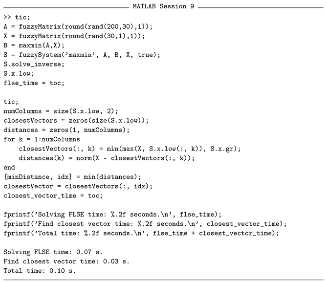
5.3. Step 6: Find the Closest Solution to the Current State

For the system (5), every interval described by the greatest solution from the right and any of its lower solutions from the left is called an interval solution. Any value inside the interval solution is still a solution of the system [1,38]. Therefore, the system (5) has as many interval solutions and as many lower solutions. In order to find the solution (as a fuzzy vector) which is closest to some other fuzzy vector (in our case, the initial control units settings), we can use the following straightforward Algorithm 2:

Algorithm 2 Find the closest solution

Step 1: Define the current sensor readings $X_0$ Step 2: FOR every interval solution $[X_{lo{w}_i},X_{gr}]$: Step 3:       Initialize a candidate solution ${\overline{X}}_i$ Step 4:       FOR every dimension (j) of the $i^{th}$ vector: Step 5:             IF $X_{0_j}$ is inside the interval $[X_{{lo{w}_i}_j},X_{g{r}_j}]$ Step 6:                   THEN $X_{0_j}$ is already in the target interval, so ${\overline{X}}_{ij}=X_{0_j}$ Step 7:                   ELSE for ${\overline{X}}_{ij}$ take either $X_{{lo{w}_i}_j}$ or $X_{{gr}_j}$, which is closer to the target ${\overline{X}}_{ij}$.                         END IF                    END FOR             END FOR Step 8: From all candidate solutions ${\overline{X}}_i$, the new $X_{new}$ is the one which is mathematically closest to the current $X_0$. I.e. select candidate solution ${\overline{X}}_i$, such that ${\sum }_j|{\overline{X}}_{i_j}-X_{0_j}|$ is minimal. Step 9: END

6. Examples and MATLAB Execution

Example 1.

Let us have a $max-min$ FLSE. Its knowledge base will be represented by the FM A:

$$A=\left(\begin{array}{ccccc}0.5& 0.6& 0.4& 0.1& 0.4\\ 0.1& 0.4& 0.1& 0.2& 0\\ 0.9& 0.5& 0.2& 0.2& 0.9\end{array}\right)$$

(7)

This system has five sensors modeling the environment status and three rules describing how the environment parameters (B) will change depending on the values (normalized as a fuzzy numbers) of the sensors (X). Each sensor reading have it’s own level of importance in each rule.

In this example, we will use the following sensor readings as a starting point for the system:

$$X=\left(\begin{array}{c}0.9\\ 0.5\\ 0.5\\ 0.3\\ 0.9\end{array}\right)$$

(8)

Let us implement Algorithm 1. We will use the software from [50] and will execute the algorithm steps in MATLAB.

6.1. Algorithm 1, Step 1—Initialize FMs

6.2. Algorithm 1, Step 2—Predict the Environment Status

The system has three environmental parameters. By executing this step, we can see in what degree every ot this parameters is currently observed.

6.3. Algorithm 1, Step 3—Define New Target System Status

Now, let us assume that we want to achieve another environment status by lowering the level of degree with which the third parameter is present ($B_3=0.9)$. Let us try with two options—$B_{{new}_1}$, and $B_{{new}_2}$—for which $b_1$ and $b_2$ will remain the same; but we will try to lower $b_3$ first to $0.4$, and then to $0.5$.

6.4. Algorithm 1, Step 4—Solve the Inverse Problem

Now, we create two FLSEs (one for $B_{{new}_1}$ and one for $B_{{new}_2}$), and solve them. The accepted parameters for the solve_inverse function are:

• The composition of the FLSE—in our case this will be $max-min$.
• The matrix A.
• The matrix B.
• The matrix X—this is what we will try to find, so we can pass an empty array here.
• A Boolean parameter to flag if we need to find the complete solution set, or just the greatest solution.

We solve both of the following systems:

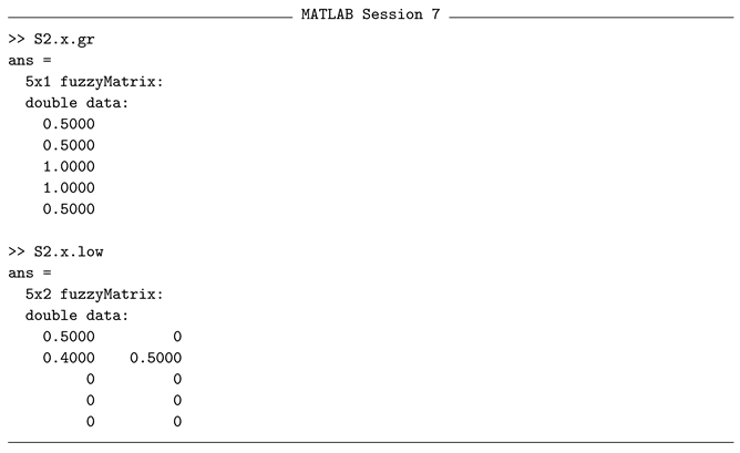
6.5. Algorithm 1, Step 5—Obtain Solutions

First, let us obtain all the solutions for $B_{{new}_1}$ (i.e., $S_1$).

For $S_1$, we can see that S1.x.exists = 0, which means that the system is inconsistent (i.e., the target environment state cannot be obtained).

For $S_2$, we can see that the system is consistent S2.x.exists = 1, and it has one greatest solution (S2.x.gr.size(2) = 1), and two lower solutions (S2.x.low.size(2) = 2).

6.6. Algorithm 1, Step 6—Check for Consistency

For the system $S_1$, we already determined that it is inconsistent, so the algorithm ends here. Further, we will focus on the system $S_2$.

6.7. Algorithm 1, Step 7—Find the New Control Units Settings

Let us print the greatest solution and all the lower solutions of the system $S_2$.

From the greatest solution and the two lower solutions, we know that the system has two interval solutions, which determine the complete solution set of $S_2$:

$$\begin{array}{c}{X}_1=\left(\begin{array}{c}0.5\\ \left[0.4,0.5\right]\\ \left[0,1\right]\\ \left[0,0.1\right]\\ \left[0,0.5\right]\end{array}\right)\end{array}{X}_2=\left(\begin{array}{c}\left[0,0.5\right]\\ 0.5\\ \left[0,1\right]\\ \left[0,1\right]\\ \left[0,0.5\right]\end{array}\right)$$

(9)

Let us find the closest to the initial X vector for both of the interval solutions:

We can see that it is the same vector for both interval solutions, so the new value for X should be the following:

$$\begin{array}{c}{X}_{new}=\left(\begin{array}{c}0.5\\ 0.5\\ 0.5\\ 0.3\\ 0.5\end{array}\right)\end{array}$$

(10)

That means that we will need to adjust just the first control unit, lowering it with $0.4$, and the last control unit, lowering it again with $0.4$. This is the minimal intervention that we can achieve in order to change the system behavior from B to $B_{{new}_2}$.

6.8. Algorithm Step 8

Depending on the real-world implementation of the system, we now need to use our actuators connected to the first and the last control units, in order to adjust them to the target values.

Example 2.

Larger system with 50 sensors and 1000 rules.

As a showcase, let us execute a larger example. The FLSE parameters here will be random and, for convenience, the full MATLAB session will be reduced to the information about the execution steps, the number of lower solutions, and the execution time.

Here, we can see that the total execution time for the whole process is 0.1 s, where the time to solve the FLSE is 0.07 s, and the time to find the minimal intervention vector is 0.03 s. As already mentioned, the execution time depends on the number of the lower solutions of the system and may vary.

Next, let us inspect the system:

The system is consistent. It has 1 greatest solution and 43 lower solutions.

7. Conclusions

In this article, a method for adjusting sensor-controlled systems with minimal intervention is presented. It facilitates the methods for solving the direct and inverse problems for fuzzy linear systems of equations (FLSEs); here, we have a generalized approach, but it should be relatively easy to use the same principles for more specific systems. Using the here-presented algorithms, we can ensure that the change we want to achieve is either not possible, or, if it is possible, then we can ensure that it is performed with the minimal possible intervention. This is ensured from the algorithms backing the process of acquiring the complete solution set of the system (5), presented in [48].

For the software implementation of the here-provided example, we use the software from [50], which is already proven to work efficiently, and has been shown to be able to find all possible lower solutions of the system—a complex, non-trivial task [3,47,48,49].

While this article is focused on a potential application of FLSEs in the area of sensor-controlled systems, it still does not provide a complete end-to-end framework for modeling such systems—a task which should be subject to thorough research and implementation in the future. Another obvious next step in this research will be to introduce a method, as well as a way to evaluate a new state of the system, which is closest but not equal to the target; this is needed in cases when a target is not possible to find (i.e., when the system (5 is not consistent).

References

1. De Baets, B. Analytical solution methods for fuzzy relational equations. In Fundamentals of Fuzzy Sets; The Handbooks of Fuzzy Sets, Series; Dubois, D., Prade, H., Eds.; Kluwer Academic Publishers: Amsterdam, The Netherlands, 2000; Volume 1, pp. 291–340. [Google Scholar]
2. Di Nola, A.; Pedrycz, W.; Sessa, S.; Sanchez, E. Fuzzy Relation Equations and Their Application to Knowledge Engineering; Kluwer Academic Press: Dordrecht, The Netherlands, 1989. [Google Scholar]
3. Peeva, K.; Kyosev, Y. Fuzzy Relational Calculus-Theory, Applications and Software (with CD-ROM). In Advances in Fuzzy Systems—Applications and Theory; World Scientific Publishing Company: Singapore, Singapore, 2004; Volume 22, Available online: https://www.mathworks.com/academia/books/fuzzy-relational-calculus-peeva.html (accessed on 23 May 2024).
4. Baldwin, J.F. Fuzzy logic and fuzzy reasoning. In Fuzzy Reasoning and Its Applications; Mamdani, E.H., Gaines, B.R., Eds.; Academic Press: London, UK, 1981. [Google Scholar]
5. Esragh, F.; Mamdani, E.H. A general approach to linguistic approximation. In Fuzzy Reasoning and Its Applications; Mamdani, E.H., Gaines, B.R., Eds.; Academic Press: London, UK, 1981. [Google Scholar]
6. Jang, J.-S.R.; Gulley, N. The Fuzzy Logic Toolbox for Use with MATLAB; MathWorks Inc.: Natick, MA, USA, 1995. [Google Scholar]
7. Mamdani, E.H.; Assilian, S. An experiment in linguist synthesis with fuzzy logic controller. Int. J. Man–Mach. Stud. 1975, 7, 1–13. [Google Scholar] [CrossRef]
8. Siler, W.; Buckley, J.J. Fuzzy Expert Systems and Fuzzy Reasoning; Wiley InterScience: Hoboken, NJ, USA, 2004. [Google Scholar]
9. Yager, R.R.; Zadeh, L.A. An Introduction to Fuzzy Logic Applications in Intelligent Systems; Kluwer Academic Publishers: Amsterdam, The Netherlands, 1991. [Google Scholar]
10. Zadeh, L.A. Making computers think like people. IEEE Spectr. 1984, 21, 26–32. [Google Scholar] [CrossRef]
11. Zahariev, Z. Fuzzy reasoning through fuzzy linear systems of equations. In Proceedings of the Technical University—Sofia; Book 3. The Technical University of Sofia Publishing House: Sofia, Bulgaria, 2010; Volume 60, pp. 58–66. [Google Scholar]
12. Kocken, H.G.; Albayrak, I. A Short Review on Fuzzy System of Linear Equations Applications. In Handbook of Research on Transdisciplinary Knowledge Generation; IGI Global: Hershey, PA, USA, 2019; pp. 75–87. [Google Scholar] [CrossRef]
13. Aviso, K.B.; Tan, R.R.; Culaba, A.B.; Cruz, J.B., Jr. Fuzzy input–output model for optimizing eco-industrial supply chains under water footprint constraints. J. Clean. Prod. 2011, 19, 187–196. [Google Scholar] [CrossRef]
14. Rahgooy, T.; Yazdi, H.S.; Monsefi, R. Fuzzy Complex System of Linear Equations Applied to Circuit Analysis. Int. J. Comput. Electr. Eng. 2009, 1, 535–541. [Google Scholar] [CrossRef]
15. Jin, Y. Advanced Fuzzy Systems Design and Applications; Physica-Verlag Heidelberg: Heidelberg, Germany, 2002. [Google Scholar]
16. Dorf, R.C.; Bishop, R.H. Modern Control Systems, 13th ed.; Pearson Education: London, UK, 2016. [Google Scholar]
17. Meijer, G.C.M. Smart Sensor Systems; John Wiley and Sons Ltd.: Hoboken, NJ, USA, 2008. [Google Scholar]
18. Merhav, S. Aerospace Sensor Systems and Applications; Springer Science & Business Media: New York, NY, USA, 2012. [Google Scholar]
19. Bolton, W. Instrumentation and Control Systems, 3rd ed.; Newnes: Oxford, UK, 2021. [Google Scholar]
20. De Silva, C.W. Sensors and Actuators: Control System Instrumentation; CRC Press: Boca Raton, FL, USA, 2007. [Google Scholar]
21. Soloman, S. Sensors and Control Systems in Manufacturing; McGraw-Hill, Inc.: New York, NY, USA, 1994. [Google Scholar]
22. Meijer, G.; Makinwa, K.; Pertijs, M. (Eds.) Smart Sensor Systems: Emerging Technologies and Applications; John Wiley and Sons Ltd.: Hoboken, NJ, USA, 2014. [Google Scholar]
23. Pal, V.C.; Ganguli, S.; Tripathi, S.L. (Eds.) Industrial Control Systems; John Wiley & Sons: Hoboken, NJ, USA, 2024. [Google Scholar]
24. Sinopoli, B.; Sharp, C.; Schenato, L.; Schaffert, S.; Sastry, S.S. Distributed control applications within sensor networks. Proc. IEEE 2003, 91, 1235–1246. [Google Scholar] [CrossRef]
25. Chen, W.; Chen, L.; Chen, Z.; Tu, S. A realtime dynamic traffic control system based on wireless sensor network. In Proceedings of the 2005 International Conference on Parallel Processing Workshops (ICPPW’05), Oslo, Norway, 14–17 June 2005; pp. 258–264. [Google Scholar] [CrossRef]
26. Jing, C.; Shu, D.; Gu, D. Design of Streetlight Monitoring and Control System Based on Wireless Sensor Networks. In Proceedings of the 2007 2nd IEEE Conference on Industrial Electronics and Applications, Harbin, China, 23–25 May 2007; pp. 57–62. [Google Scholar] [CrossRef]
27. Zhou, Y.; Yang, X.; Guo, X.; Zhou, M.; Wang, L. A Design of Greenhouse Monitoring & Control System Based on ZigBee Wireless Sensor Network. In Proceedings of the 2007 International Conference on Wireless Communications, Networking and Mobile Computing, Shanghai, China, 21–25 September 2007; pp. 2563–2567. [Google Scholar] [CrossRef]
28. Yang, S.-H.; Cao, Y. Networked Control Systems and Wireless Sensor Networks: Theories and Applications. Int. J. Syst. Sci. 2008, 39, 1041–1044. [Google Scholar] [CrossRef]
29. Kim, Y.; Evans, R.G.; Iversen, W.M. Remote Sensing and Control of an Irrigation System Using a Distributed Wireless Sensor Network. IEEE Trans. Instrum. Meas. 2008, 57, 1379–1387. [Google Scholar] [CrossRef]
30. Suh, C.; Ko, Y.-B. Design and implementation of intelligent home control systems based on active sensor networks. IEEE Trans. Consum. Electron. 2008, 54, 1177–1184. [Google Scholar] [CrossRef]
31. Park, D.-H.; Park, J.-W. Wireless Sensor Network-Based Greenhouse Environment Monitoring and Automatic Control System for Dew Condensation Prevention. Sensors 2011, 11, 3640–3651. [Google Scholar] [CrossRef]
32. Yedavalli, R.K.; Belapurkar, R.K. Application of wireless sensor networks to aircraft control and health management systems. J. Control Theory Appl. 2011, 9, 28–33. [Google Scholar] [CrossRef]
33. Li, M.; Lin, H.-J. Design and Implementation of Smart Home Control Systems Based on Wireless Sensor Networks and Power Line Communications. IEEE Trans. Ind. Electron. 2015, 62, 4430–4442. [Google Scholar] [CrossRef]
34. Lu, C.; Saifullah, A.; Li, B.; Sha, M.; Gonzalez, H.; Gunatilaka, D.; Wu, C.; Nie, L.; Chen, Y. Real-Time Wireless Sensor-Actuator Networks for Industrial Cyber-Physical Systems. Proc. IEEE 2016, 104, 1013–1024. [Google Scholar] [CrossRef]
35. Mekki, M.; Abdallah, O.; Amin, M.B.M.; Eltayeb, M.; Abdalfatah, T.; Babiker, A. Greenhouse monitoring and control system based on wireless Sensor Network. In Proceedings of the 2015 International Conference on Computing, Control, Networking, Electronics and Embedded Systems Engineering (ICCNEEE), Khartoum, Sudan, 7–9 September 2015; pp. 384–387. [Google Scholar] [CrossRef]
36. Khan, M.; Silva, B.N.; Han, K. A Web of Things-Based Emerging Sensor Network Architecture for Smart Control Systems. Sensors 2017, 17, 332. [Google Scholar] [CrossRef] [PubMed]
37. Lakhiar, I.A.; Jianmin, G.; Syed, T.N.; Chandio, F.A.; Buttar, N.A.; Qureshi, W.A. Monitoring and Control Systems in Agriculture Using Intelligent Sensor Techniques: A Review of the Aeroponic System. J. Sens. 2018, 2018, 8672769. [Google Scholar] [CrossRef]
38. Peeva, K.; Zaharieva, G.; Zahariev, Z. Resolution of max-t-norm fuzzy linear system of equations in BL-algebras. AIP Conference Proceedings 2016, 1789, 060005. [Google Scholar] [CrossRef]
39. Markovskii, A. On the relation between equations with max-product composition and the covering problem. Fuzzy Sets Syst. 2005, 153, 261–273. [Google Scholar] [CrossRef]
40. Peeva, K. Universal algorithm for solving fuzzy relational equations. Italian Journal of Pure and Applied Mathematics 2006, 19, 169–188. [Google Scholar]
41. Peeva, K. Resolution of Fuzzy Relational Equations—Method, Algorithm and Software with Applications. Information Sciences 2013, 234, 44–63. [Google Scholar] [CrossRef]
42. Ignjatović, J.; Ćirić, M.; Šešelja, B.; Tepavčević, A. Fuzzy relational inequalities and equations, fuzzy quasi-orders, closures and openings of fuzzy sets. Fuzzy Sets Syst. 2015, 260, 1–24. [Google Scholar] [CrossRef]
43. Yang, S. Some Results of the Fuzzy Relation Inequalities With Addition–Min Composition. IEEE Trans. Fuzzy Syst. 2018, 26, 239–245. [Google Scholar] [CrossRef]
44. Yang, X. Solutions and strong solutions of min-product fuzzy relation inequalities with application in supply chain. Fuzzy Sets Syst. 2020, 384, 54–74. [Google Scholar] [CrossRef]
45. Zahariev, Z.; Zaharieva, G.; Peeva, K. Fuzzy relational equations—Min-Goguen implication. AIP Conf. Proc. 2022, 2505, 120004. [Google Scholar] [CrossRef]
46. Zahariev, Z. Software for solving fuzzy relational equations in BL-algebras. AIP Conf. Proc. 2023, 2939, 030012. [Google Scholar] [CrossRef]
47. Peeva, K. Finite L-Fuzzy Machines. Fuzzy Sets Syst. 2004, 141, 415–437. [Google Scholar] [CrossRef]
48. Zahariev, Z. Solving max–min Relational Equations. Software and Applications. In Proceedings of the International Conference “Applications of Mathematics in Engineering and Economics (AMEE’08)”, AIP Conference Proceedings, Sozopol, Bulgaria, 8–14 June 2008; Venkov, G., Kovatcheva, R., Pasheva, V., Eds.; American Institute of Physics: Melville, NY, USA, 2008; Volume 1067, pp. 516–523. [Google Scholar]
49. Zahariev, Z. Software package and API in MATLAB for working with fuzzy algebras. In Proceedings of the International Conference “Applications of Mathematics in Engineering and Economics (AMEE’09)”, AIP Conference Proceedings, Sozopol, Bulgaria, 7–12 June 2009; Venkov, G., Kovatcheva, R., Pasheva, V., Eds.; American Institute of Physics: Melville, NY, USA, 2009; Volume 1184, pp. 350–434, ISBN 978-0-7354-0750-9. [Google Scholar]
50. Zahariev, Z. (Most Recent Update). 2024. Available online: https://www.mathworks.com/matlabcentral/fileexchange/27046-fuzzy-calculus-core-fc2ore (accessed on 26 May 2024).
51. Sanchez, E. Resolution of composite fuzzy relation equations. Inf. Control 1976, 30, 38–48. [Google Scholar] [CrossRef]