Large-Eddy Simulations of a Supersonic Impinging Jet Using OpenFOAM

Abstract

Supersonic impinging jets are a versatile configuration that can model the compressible flows of cold-spray manufacturing and vertical take-off-and landing strategy. In this work, rhoCentralFoam, solver of the OpenFOAM framework, and a large-eddy simulation formulation were used to simulate an underexpanded supersonic jet of Mach $1.45$ and nozzle pressure ratio of 4, impinging on a flat wall situated at $1.5$ nozzle diameters away from the jet outlet. Care was taken in the mesh construction to properly capture the characteristic standoff shock and vortical structures. The grid convergence index was evaluated with three meshes of increasing spatial resolution. All meshes can generally be considered as sufficient in terms of results focused on time-averaged values and mean physical properties such as centerline Mach number profile. However, the highest resolution mesh was found to capture fine shear vortical structures and behaviors that are absent in the coarser cases. Therefore, the notion of adequate grid convergence may differ between analyses of time-averaged and transient information, and so should be determined by the user’s intention for conducting the simulations. To guide the selection of mesh resolution, scaling analyses were performed, for which the current rhoCentralFoam solver displays a good weak scaling performance and maintains a linear strong scaling up to 4096 cores (32 nodes) for an approximately 40 million-cell mesh. Due to the internode communication bottlenecks of OpenFOAM and improvements in central processing units, this work recommends, for future scaling analyses, adopting a “cells-per-node” basis over the conventional “cells-per-core” basis, with particular attention to the interconnect speed and architecture used.

1. Introduction

Supersonic impinging jets (SIJs) play a pivotal role in numerous engineering applications, ranging from industrial processes such as cold-spray manufacturing [1] to aerospace systems such as vertical take-off and landing thrusters [2]. Hence, there is value in studying and understanding the complex flow phenomena associated with an SIJ as it can be used to guide the optimization of various applications.

Despite decades of extensive experimental research in this field [2,3,4,5,6,7,8], high-speed cameras and the particle image velocimetry technique are still insufficient in capturing the megahertz sampling frequencies required for the highly transient shock structures of the SIJ configuration, which arise from its interactions with the compressible jet shear layer [9,10,11,12]. Consequently, computational fluid dynamics (CFD) simulations to augment experimental SIJ research efforts have been used for more than 20, demonstrating that, for SIJ configurations, steady mean numerical results from the Reynolds-averaged Navier–Stokes (RANS) methodology can have good overall agreement with physical measurements [5,13]. Li et al. [1] even extended their validated mean flow results with a Lagrangian module for particle motion to study gas–particle interactions during the steady cold-spray process. Recognizing the highly transient characteristics of SIJs, Dauptain and co-workers [14] employed the inherently unsteady large-eddy simulation (LES) formulation on the SIJ configuration of Henderson et al. [6], establishing that, for an explicit third-order solver with an unstructured mesh, more than 20M cells are required to ensure grid convergence. The advantages of LES over RANS for SIJ simulations were further highlighted by Chan et al. [15], even though both methods were found to be able to capture the mean flow features. While useful in supplementing experiments, CFD simulations have previously not been able to provide high-fidelity results at a tractable cost. However, the advancements in highly scalable high-performance computing (HPC) resources and the development of accurate and computationally efficient CFD solvers render the time right to conduct comprehensive numerical studies of the SIJ configuration, as seen in the recent intensive yet insightful studies in References [16,17], with the latter even including heat transfer effects.

Regarding CFD solvers for transient compressible flows like the SIJ configuration, there are in general three categories, namely, commercial, in-house, and open-source. Typically well validated and widely used for engineering problems, commercial CFD solvers like ANSYS Fluent [18,19] and Simcenter STAR-CCM+ [20,21] offer the advantages of direct support for troubleshooting, user-friendly graphical user interfaces, and solver runtime stability. There are, however, two main drawbacks. First, most commercial CFD software suites do not expose any of the underlying code being used, so there is no way for users to directly modify the algorithms or inspect the mathematics and logic, except for relying on documentation and the word of the developers. Second, the cost for even a basic-level solver license can be prohibitive, and now is usually coupled with a trend to lock each license to a certain CPU core count, which is restrictive for high-fidelity simulations.

The traditional route to circumvent the limitations of commercial CFD solvers, especially in the academic community, is to develop in-house and purpose-built CFD code [1,5,10,14,17,22]. Not accounting for the time and effort needed for such developments, which are usually daunting and specialized, the cost of in-house CFD solvers is often minimal. Nonetheless, they are typically exclusive to the developers, inconsistent in documentation and support, and validated for only specific configurations. Furthermore, legacy solvers that are not regularly maintained may face scalability issues with constantly upgrading HPC systems.

Compared to commercial and in-house CFD solvers, open-source CFD solvers have previously been the least common, mostly due to a lack of validation studies and existing literature [23]. However, with the introduction of the OpenFOAM (Open Field Operation And Manipulation) framework in 2004 [24], along with its built-in libraries and support for user modifications [25,26,27], open-source solvers have generally garnered much more acceptance. To date, among the various open-source CFD solvers available, the OpenFOAM framework [28] remains a popular choice for compressible, turbulent SIJ simulations [15,16,25], owing to its flexibility, extensibility, and robustness [29,30,31,32].

For the above reasons, this paper considers large-eddy simulations of SIJs using the rhoCentralFoam solver within the OpenFOAM framework. In particular, the focus was placed on SIJs with a separation distance (i.e., distance between jet nozzle and wall) of less than two nozzle diameters, a scenario that has been found to be lacking in the existing computational literature except for such studies as References [1,15]. Such close separation distances are of particular interest because the stability (or lack thereof) of the standoff shock, located just above the wall, is very sensitive to both the nozzle pressure ratio, $\mathrm{NPR}$, and the separation distance [33]. This observation applies not only to the magnitude of unsteadiness, but also the various modes of unsteadiness such as the typical jittering and more abrupt and larger jumps in the standoff shock location [34].

The remainder of this paper is structured as follows: In the next section, the methodology is communicated, providing information on the mesh topology, initial and boundary conditions, CFD schemes and models, and HPC configurations. Then, the results are discussed in terms of grid convergence, effects of mesh resolution, simulation accuracy, and solver scalability on the given HPC architectures. Conclusions are provided at the end.

2. Methodology

2.1. Configuration and Mesh Topology

The investigated configuration consists of an impingement jet that originates from a nozzle of diameter $D=12.7\mathrm{mm}$ and with a separation distance of $H=1.5D$. With a Mach number, $\mathrm{Ma}$, of $1.45$ and an $\mathrm{NPR}=4$, the jet is supersonic and underexpanded. Figure 1 depicts the ${\lambda }_2$ isosurface, which shows turbulent features, and the mid-plane of the Mach number contour, which demarcates the supersonic jet core, of the SIJ configuration at an instant in the quasi-steady state. The overall domain dimensions were set with radial and streamwise extents of $10D$ and $4.5D$, respectively, with the domain inlet positioned $1.5D$ above the flat wall.

Figure 1. Illustration of the SIJ configuration with ${\lambda }_2$ isosurface and mid-plane colored by Mach number at quasi-steady state.

Figure 1. Illustration of the SIJ configuration with ${\lambda }_2$ isosurface and mid-plane colored by Mach number at quasi-steady state.

Recognizing the advantages of a fully structured hexahedral mesh over an unstructured tetrahedral mesh, which include lower numerical diffusion, higher overall accuracy, and better cell coverage efficiency, the computational domain in this study was carefully discretized by a two-step approach:

• A two-dimensional slice of the mesh was generated with a user-defined number of cells and grading tailored to resolve regions of complex flow and particular interest, such as the jet shear and wall boundary layers, as well as the standoff shock, with higher fidelity. As shown in Figure 2, these regions notably include the nozzle lip, jet shear layer proximity, and zone adjacent to the wall. The cell gradients were specified by defining the desired cell spacing and number of nodes along the wall-normal direction, and utilizing the monotonic rational quadratic spline spacing function.
• A three-dimensional mesh was generated by specifying the number of rotational steps around the axis (i.e., the centerline of the two-dimensional slice) to achieve the required angular dimension of the cell size. At this stage, an axisymmetric cylindrical mesh formed by an O-grid has been generated. However, a singular point will be created in the middle of the mesh and must be resolved, which was achieved via the insertion of an H-grid in the jet core region.

The resulting OH-grid, as shown in Figure 3, offers several benefits. First, it creates consistently high-quality cells near the walls that enable the precise matching of the circular nozzle. This match is crucial for the accurate capturing of the boundary layer phenomena and flow interactions. Moreover, the OH-grid facilitates smooth gradient transitions from the near-wall region towards the jet core and further into the far-field. This seamless transition is essential for maintaining numerical stability and resolving flow features across the entire computational domain.

Figure 2. Zoomed-in view of the two-dimensional slice to illustrate cell grading applied to the nozzle wall and lip, jet shear layer, and boundary layer of the impinged wall.

Figure 2. Zoomed-in view of the two-dimensional slice to illustrate cell grading applied to the nozzle wall and lip, jet shear layer, and boundary layer of the impinged wall.

To facilitate essential grid convergence studies, three meshes of varying cell counts were generated by varying the maximum cell size within the jet core in both the streamwise and radial directions (i.e., along the x- and y-axes, respectively). The angular resolution of the meshes was also varied by decreasing the size of each rotational step. For ease of comparison, the specifics of the three meshes are given side by side in

Table 1. Specifications of the three levels of mesh resolution.

	Coarse	Medium	Fine
Maximum jet core cell size	$D/60$	$D/80$	$D/100$
Minimum impinged wall cell size	$D/600$	$D/800$	$D/1000$
Minimum nozzle lip cell size	$D/3000$	$D/4000$	$D/4000$
Angular size	$2^{\circ }$	$1.5^{\circ }$	$1^{\circ }$
Total cell count	$N3=$ 8,469,000	$N2=$ 17,700,000	$N1=$ 40,986,000
Cell ratio	0.207	0.432	1

.

2.2. Initial and Boundary Conditions

The nozzle inlet condition was matched to the conditions experimentally tested in Reference [34] using the “fixedValue” option for the velocity condition, and “totalPressure” and “totalTemperature” options for the pressure and temperature conditions, respectively. The jet was exhausted into a domain initialized to ambient air conditions of 101,325 $\mathrm{Pa}$ and $300\mathrm{K}$. Both the impinged and nozzle walls were set to the “noSlip” boundary condition and fixed at $300\mathrm{K}$. The Reynolds number with reference to the nozzle exit velocity and nozzle diameter was $Re=3.61\times {10}^5$. The “waveTransmissive” boundary condition is important in the accurate simulation of compressible flows where wave reflections and transmissions at the domain outlets are significant. This boundary condition enables the solver to capture the propagation of acoustic and pressure waves through the computational domain with minimal artificial reflections, ensuring that unbounded flow domains are realistically represented. The specific values prescribed to the boundary conditions are given in

Table 2. Boundary conditions applied.

Patch	Velocity $[\mathbf{m}/\mathbf{s}]$	Pressure $\left[\mathbf{Pa}\right]$	Temperature $\left[\mathbf{K}\right]$
Inlet 1	fixedValue: $422.4$	totalPressure: 405,300	totalTemperature: 300
Outlet 1	waveTransmissive	waveTransmissive: 101,325	waveTransmissive
Walls	noSlip	zeroGradient	fixedValue: 300

¹ “gamma” of $1.4$ was used where applicable.

.

2.3. CFD Solver

In this work, rhoCentralFoam, a transient, density-based flow solver of the default OpenFOAM package from ESI-group [28], was employed for two main reasons. First, rhoCentralFoam has a general second-order accuracy due to its incorporation of the central-upwind scheme by Kurganov and Tadmor [35]. Second, rhoCentralFoam has a built-in shock-capturing module that has demonstrated the ability to accurately capture various shock structures in well-studied cases like shock diamonds in freely exhausting jets and supersonic flow over various canonical solid bodies [36,37]. In fact, rhoCentralFoam has been validated over a wide range of low to medium supersonic Mach numbers [32].

For all simulations, the second-order Crank–Nicholson time scheme was selected as it has been shown to provide a good combination of accuracy and stability [16] as compared to the first-order Euler scheme or backwards scheme. The timestep size of the simulation was allowed to be adjusted such that the Courant–Friedrichs–Lewy number (CFL) did not exceed 0.3, which was found to provide sufficient numerical stability.

Regarding transport models, the Sutherland formulation [38] was applied to describe the dependence of dynamic viscosity on temperature. Thermal diffusivity was computed from the dynamic viscosity through a prescribed constant Prandtl number of $0.71$.

2.4. LES Formulation

Turbulence can be described as a cascade of energy in the form of large-scale vortices progressively decaying into smaller vortices down to the smallest length scale, known as the Kolmogorov scale, for the given flow scenario [39]. To resolve all scales is generally intractable for practical engineering problems [40], so LES was selected for this work. In LES, the larger scales that contain most of the energy are directly solved, while scales not resolved by the implemented mesh resolution are modeled. The typical assumption for subgrid-scale models is that the unresolved scales serve primarily to dissipate energy from the larger scales through the cascade process. Therefore, LES can be thought of as a form of spatial filtering where flow length scales less than the filtered length scale are modeled by a turbulence model. For this study, the filtered compressible conservation equations of the LES formulation were solved with a k-equation eddy viscosity model for turbulence closure. As the governing equations have been given in multiple previous works, like Reference [16], they will not be repeated here for brevity.

Considering practicality, one may argue that the unsteady Reynolds-averaged Navier–Stokes (URANS) formulation is also able to accurately predict key bulk flow properties, such as centerline velocity profiles and mean standoff shock distance, but at lower computational costs than LES. However, the shock structures from URANS simulations performed at the earlier stage of this work were found to be less defined than those from LES, which is an observation that may be attributed to the inaccurate modeling of critical regions like the jet shear layer and wall boundary layer [15]. Moreover, as the mesh resolution increases, the timestep size has to decrease to maintain a target CFL, which in turn reduces the computational efficiency of the URANS formulation. Hence, contrary to popular belief, the computation time required for URANS and LES simulations is actually comparable in high-speed flow cases, thus removing the primary advantage of using the former and justifying the choice to use the latter in this study.

2.5. HPC Setup

All simulations were conducted on the high-performance computing infrastructure of the Aspire2A cluster of the National Supercomputing Center Singapore. Each standard computational node features dual AMD EPYC™ 7713 CPUs, providing a total of 128 cores and 512 GB of available RAM. The interconnected network architecture utilizes a Hewlett Packard Enterprise Slingshot Interconnect with the Dragonfly Topology configuration [41], which facilitates efficient communication between nodes with a maximum bandwidth capability of up to 200 Gbits/s.

3. Results and Discussion

3.1. Grid Convergence Analysis

The mean centerline Mach number profiles for the three levels of mesh resolution are depicted in Figure 4, where each can be divided into four distinct segments:

• Up to $x/D=0.4$, no shock structure has formed yet so all three cases are in near perfect agreement since the flow is laminar and relatively unperturbed.
• In the second segment, all cases exhibit a peak Mach number of approximately 2 at around $x/D=0.75$. More specifically, between the medium and fine cases, the deviations in peak Mach number and its location are both approximately 2%, which are marginally smaller than the 3% and 2% differences in peak Mach number and its location, respectively, between the coarse and fine cases.
• The third segment primarily captures the range where the standoff shock oscillates, and the convergence over the three meshes is less clear and mixed.
• In the final segment, which corresponds to the high pressure recirculating flow, the fine mesh shows a distinctively higher decelerating Mach number profile than the coarse and medium meshes, though all cases converge to zero Mach number at $x/D=1.5$ due to the no-slip wall condition.

To systematically assess the convergence behavior of the three SIJ simulations at different mesh resolutions, the grid convergence index ($\mathrm{GCI}$) evaluation [42,43] was performed. The GCI results are shown in

Table 3. GCI evaluation [42,43] of coarse, medium, and fine SIJ simulations. See Reference [43] for further information on the parameters.

Parameter	Value
$N1$, $N2$, $N3$	40,986,000, 17,700,000, 8,469,000
${\varphi }_1$, ${\varphi }_2$, ${\varphi }_3$	$2.05$, $2.01$, $1.99$
$r_{21}={(N1/N2)}^{1/3}$, $r_{32}={(N2/N3)}^{1/3}$	$1.32$, $1.28$
${\epsilon }_{21}={\varphi }_2-{\varphi }_1$, ${\epsilon }_{32}={\varphi }_3-{\varphi }_2$	$-0.04$, $-0.02$
$e_a^{21}=|({\varphi }_1-{\varphi }_2)/{\varphi }_1|$	1.95%
p	$1.89$
$e_{\mathrm{ext}}^{21}$, $e_{\mathrm{ext}}^{32}$	2.75%, 1.65%
${\mathrm{GCI}}_{\mathrm{fine}}^{21}$	3.53%

, where ${\varphi }_1$, ${\varphi }_2$, and ${\varphi }_3$ refer to the peak mean centerline Mach number values (see Figure 4) of the fine, medium, and coarse cases, respectively. In particular, the apparent order, p, given by the implicit equation

$$p=\frac{1}{log\left(r_{21}\right)}\left|log\left|\frac{{\epsilon }_{32}}{{\epsilon }_{21}}\right|+log\left(\frac{r_{21}^p-\mathrm{sgn}({\epsilon }_{32}/{\epsilon }_{21})}{r_{32}^p-\mathrm{sgn}({\epsilon }_{32}/{\epsilon }_{21})}\right)\right|=1.89,$$

is slightly lower than 2, which is aligned with the second-order spatial and temporal schemes that have been used (see Section 2.3). Furthermore, the small fine-grid convergence index, ${\mathrm{GCI}}_{\mathrm{fine}}^{21}$, given by

$${\mathrm{GCI}}_{\mathrm{fine}}^{21}=\frac{1.25e_a^{21}}{r_{21}^p-1}=0.0353,$$

suggests that the fine-grid results have a numerical uncertainty of 3.53% (not accounting for modeling errors). Combined with the marginal extrapolated relative errors, $e_{\mathrm{ext}}^{21}$ and $e_{\mathrm{ext}}^{32}$, which are computed by

$$e_{\mathrm{ext}}^{21}=\left|\frac{{\varphi }_{\mathrm{ext}}^{21}-{\varphi }_1}{{\varphi }_{\mathrm{ext}}^{21}}\right|=0.0275,e_{\mathrm{ext}}^{32}=\left|\frac{{\varphi }_{\mathrm{ext}}^{32}-{\varphi }_2}{{\varphi }_{\mathrm{ext}}^{32}}\right|=0.0165,$$

where ${\varphi }_{\mathrm{ext}}^{ji}=(r_{ji}^p{\varphi }_i-{\varphi }_j)/(r_{ji}^p-1)$, one can deduce that even the coarse mesh has converged based on its peak centerline Mach number value. In other words, all three levels of mesh resolution are adequate for the representation of time-averaged flow properties. A similar conclusion has been drawn by Dauptain et al. [14], even though the current work considers a separation distance that is more than 60% smaller.

3.2. Verification of Results

To verify the simulations, schlieren images from previous experiments [34] of a similar setup were selected. The experiment comprises a converging–diverging nozzle with a design mach number of $\mathrm{Ma}=1.45$ driven using a compressed-air-based blowdown facility in a controlled environment. In Figure 5, an instantaneous experimental schlieren image (top) and a representative numerical schlieren snapshot (bottom) are presented. Following convention, the result from the medium SIJ case was used since, as discussed in Section 3.1, all three meshes are comparable in capturing the bulk flow properties.

From Figure 5, the measured and simulated standoff shocks were observed to be located at approximately $0.35D$ and $0.47D$, respectively, above the impinged wall. This difference of ∼30% is reasonable considering that its absolute value is approximately $2\mathrm{mm}$, which is within the uncertainty of experimental schlieren imaging. Moreover, the numerical setup differs from the experiment in two ways. First, is the use of a perfectly uniform inlet condition, which will neglect boundary layer effects from the inner wall of the nozzle that would be present in experiments. Second, because of their high computational costs, the numerical simulations were run only up to milliseconds in time, in contrast to the experimental images that were several seconds after initialization of the jet. Despite these discrepancies, both sets of schlieren images illustrate a similar overall shape of the standoff shock and other flow features, as well as comparable thickness and size of the standoff shock, thus providing the necessary verification of the SIJ simulation results of this study and justification to use them in the subsequent analyses.

3.3. Effects of Mesh Resolution

While time-averaged profiles are equally captured by all three mesh resolutions of this study (see Section 3.1), the same cannot be said for transient behaviors like the standoff shock oscillations and shear-layer instabilities. To illustrate this point, Figure 6 compares the SIJ results obtained from the coarse, medium, and fine meshes at six timesteps, focusing in particular on the jet shear-layer vortices, which are seen in the middle of each subplot.

All three cases display almost identical results at the start of the simulation (i.e., $t\le 50\mathsf{\mu }\mathrm{s}$), particularly before the bow shock from the supersonic starting jet is reflected off the wall and interacts with the starting vortex ring. However, as the reflected bow shock approaches the nozzle lip at approximately $t=90\mathsf{\mu }\mathrm{s}$, differences in the jet shear layer become apparent, with small but noticeable shear instabilities being observed in the fine and medium cases, while the coarse case still appears mostly unperturbed. After the bow shock impacts the nozzle lip, shear instabilities are instantly amplified and, at the earlier stage like $t=125\mathsf{\mu }\mathrm{s}$, larger-scale vortices (enclosed by solid box) are resolved similarly by all three cases, but the intensity of smaller-scale instabilities (highlighted by dashed box) clearly increases with mesh resolution. The differences in these transient features compound over time such that for $t\ge 550\mathsf{\mu }\mathrm{s}$, as the flow has settled into a quasi-steady state, even the major unsteady flow features begin to deviate across the three cases, including the large-scale shear-layer vortices and standoff shock location (relative to the mean standoff shock height indicated by the red vertical line). Hence, the equivalence of the three meshes is only true statistically wherein any temporal dependence will be eliminated by time-averaging, an effect that is supported by the comparison of RANS and LES of SIJs by Chan et al. [15]. In turn, mean results will tend to require less mesh resolution to be captured, which is the main contributing factor to the typically lower computational cost of RANS simulations than that of URANS and LES.

To further illustrate the connection between the mesh resolution and the extent of resolved flow structures, transient pressure data from all three meshes were probed at a sampling frequency of $1\mathrm{MHz}$ from $[x,r]=[0.5D,0.5D]$ over a duration of $1\mathrm{ms}$ within the quasi-steady state. The probing location was chosen because, as seen in Figure 6, it sits within the jet shear layer and is sufficiently away from the nozzle lip so that the vortices have begun to roll up, but not so far downstream as to encounter the standoff or tail shocks. Subsequently, the pressure datasets were processed with Welch fast Fourier transform [44] using a 150-frame Hanning window with 50% overlap, producing the power spectrum density plot given in Figure 7.

Notably, the primary peak of all three cases occurs at a similar Strouhal number $\mathrm{St}\approx 1$, indicating that the largest transient features are well captured by all three levels of mesh resolutions. However, in general, as the mesh resolution increases, the energy is higher and dissipates at a slower rate, suggesting that more fine-scale structures are resolved by the increased mesh resolution, a differentiation that is especially clear for the fine mesh, as seen in Figure 6. Likely due to these differences in the smaller-scale transient features, the cascading interactions from the large to the small scale and backscattering from the small to the large scale deviate between the coarser cases and the fine case, resulting in a slight shift in the second peak of the fine mesh to $\mathrm{St}\approx 2.6$, such that the coarse and medium meshes agree better at $\mathrm{St}\approx 2$. This deviation is not statistically significant since all three meshes were found to be adequate for time-averaged properties in Section 3.1. Overall, the coarse mesh displays significant deviations from the medium and fine cases in terms of the power magnitude, even at the lower frequencies, with the deviations increasing as $\mathrm{St}$ increases. In contrast, the medium- and fine-mesh results agree reasonably well until the higher range of $\mathrm{St}\ge 5$, where the energy of the medium case decays more rapidly than that of the fine case.

3.4. Computational Scaling

From Section 3.1 and Section 3.2, one can infer that any one of the coarse, medium, or fine meshes, which have a total cell count ratio of approximately 5 over the two extremes, is sufficient to capture the bulk properties of the SIJ configuration like centerline velocity and standoff shock position, especially if they are averaged over time. Hence, for engineering evaluations where the mean information (i.e., the net effects) is often more useful than transient behaviors, the coarse SIJ case, or even RANS, can suffice. On the other hand, studies that inherently need high-fidelity representation of the temporal phenomena, such as shear-layer instabilities or jet/shock interactions, may necessitate higher mesh resolutions like the fine SIJ mesh or beyond. Therefore, the decision on the adequacy of a mesh resolution is highly dependent on the objectives of the simulation. Consequently, understanding the scalability of a solver is important as it allows for the possibility to trade runtime with CPU count, thus maintaining the same computational rate for different levels of mesh resolution.

Solver scalability has a direct impact on the efficient utilization of computational resources. It allows for the assessment of how well a solver framework can handle increasing computational loads due to a higher mesh resolution or larger computational domain. Efficient computational scaling ensures that the computational cores or compute nodes are effectively distributed and utilized, thus enabling results to be obtained within an optimal timeframe and maximizing the value of the simulations conducted. The evaluation of solver scalability is typically evaluated by using a speedup factor, $S_n$, which is defined as

$$S_n=\frac{T_1}{T_n},$$

where $T_n$ is the computing time on n core(s).

3.4.1. Weak Scaling

Weak scaling in the context of CFD is a metric used to assess the ability of the solver framework to maintain a consistent level of computational effort per core as the problem size grows by an increase in mesh resolution or computational domain size. Specifically, as the number of computational cores or nodes increases proportionally with the size of the simulated domain or mesh, the total computational workload remains constant per core. Achieving good weak scaling implies that the solver framework can effectively distribute and manage the computational tasks across multiple processors, thereby maintaining performance and efficiency even with larger and more complex simulations without potential bottlenecks such as core load imbalances. In other words, the evaluation of weak scaling provides insights into the parallel efficiency of the solver framework, allowing for the determination of an optimal simulation size and fidelity for a given amount of computational resources.

The weak scaling tests were carried out with the three meshes previously described (see Table 1). The number of cores and nodes utilized were scaled down proportionally with the number of cells for each case such that the cells-per-core count was maintained at approximately 10,000. All cases were started at the same $0.1\mathrm{ms}$ instant and run for 230,000 iterations. The compute time needed for each case relative to that of the fine case was used to calculate the speedup results presented in

Table 4. Weak scaling analysis for the three SIJ cases. Note that all presented ratios are relative to the fine case.

	Coarse	Medium	Fine
Cells per core	9452	9877	10,006
Core count	896	1792	4096
Core ratio	0.219	0.438	1
Speedup ratio	0.95	1.24	1

since the same simulations would not have been accomplished serially within a reasonable timeframe.

The weak scaling results in Table 4 show good scalability with problem size because by increasing the core count by the same factor as the cell ratio across the three cases, the speedup ratio holds relatively constant at 1. Still, further investigation into the compiler and MPI tasks with time profiling of these operations will be useful in providing explanations into specific bottlenecks, such as excessive overheads, load imbalances, or sub-optimal MPI routines. These results would be useful to guide any future work with similar parameters on the optimal computational resources required for a desired amount of compute time given a computational domain and its resolution.

3.4.2. Strong Scaling

Strong scaling is a crucial metric in CFD applications as it measures how effectively the computational workload can be distributed across additional processors to accelerate the simulation process of a constant problem size (i.e., same computational domain and mesh resolution). In other words, strong scaling indicates the turnaround time of simulations and access rate to results. By running simulations within the linear part of strong scaling, the cost-effectiveness of the simulations is maximized.

For the strong scaling analysis, only the coarse and fine meshes were studied to represent the extremes where the internode bandwidth can be a limiting factor and the cell count may saturate the CPU, respectively. In cases where 32 and 64 cores were used, a full compute node with 128 cores was allocated, but constrained to 32 and 64 MPI threads, respectively, to ensure that no other jobs were allocated to the compute node and potentially split unequally. One side effect of this allocation is that the results for the 32 and 64 cores are not exactly representative of 32- and 64-core nodes. Nonetheless, the results were still included since they can serve as indicators for strong scaling at lower core counts.

The strong scaling results are presented in Figure 8, where the baseline speedup performance is taken from the 128-core run (i.e., one full node). The ideal performance line scales proportionally with the amount of computational resources allocated (i.e., an order increase in core/node count will return an order increase in speedup). Refer to

Table 5. Strong scaling for 1, 2, 4, 8, 16, and 32 nodes (128 cores/node) for coarse and fine cases.

Node Count	Core Count, n	${\mathit{S}}_{\mathit{n}}/{\mathit{S}}_{128}$
		Coarse	Fine
1	32	0.36	0.35
	64	0.63	0.62
	128	1	1
2	256	1.78	1.52
4	512	4.21	2.90
8	1024	9.62	6.31
16	2048	19.4	14.1
32	4096	30.7	28.0

for the exact values for the strong scaling analysis.

From Figure 8, similar linear scaling is observed for a majority of the coarse and fine results. For the coarse case, linear scaling ranges from 256 to 2048 cores (2 to 16 nodes), after which speedup seems to taper off, possibly attributable to overhead intercommunication and other input/output tasks like writing of data. In contrast, the fine case displays linear scaling up to 4096 cores (32 nodes). Improvement in strong scaling due to upgraded HPC architecture can be inferred by comparison with a previous study [32], which found linear strong scaling of rhoCentralFoam to last only up to 288 cores when simulating a comparable configuration (i.e., a freely exhausting supersonic jet with 24 million cells) as in the current fine SIJ case, but on last-generation 24-core nodes.

Notably, both cases even exhibit better-than-ideal scaling performance in the 32- and 64-core runs, which is likely due to the additional cache and memory allocation from the MPI threads constraint. The superior performance of the coarse case between the 512- and 2048-core runs (4 and 16 nodes) suggests an optimal cache usage per thread for the current OpenFOAM framework under the given workload of the coarse case [45].

4. Conclusions

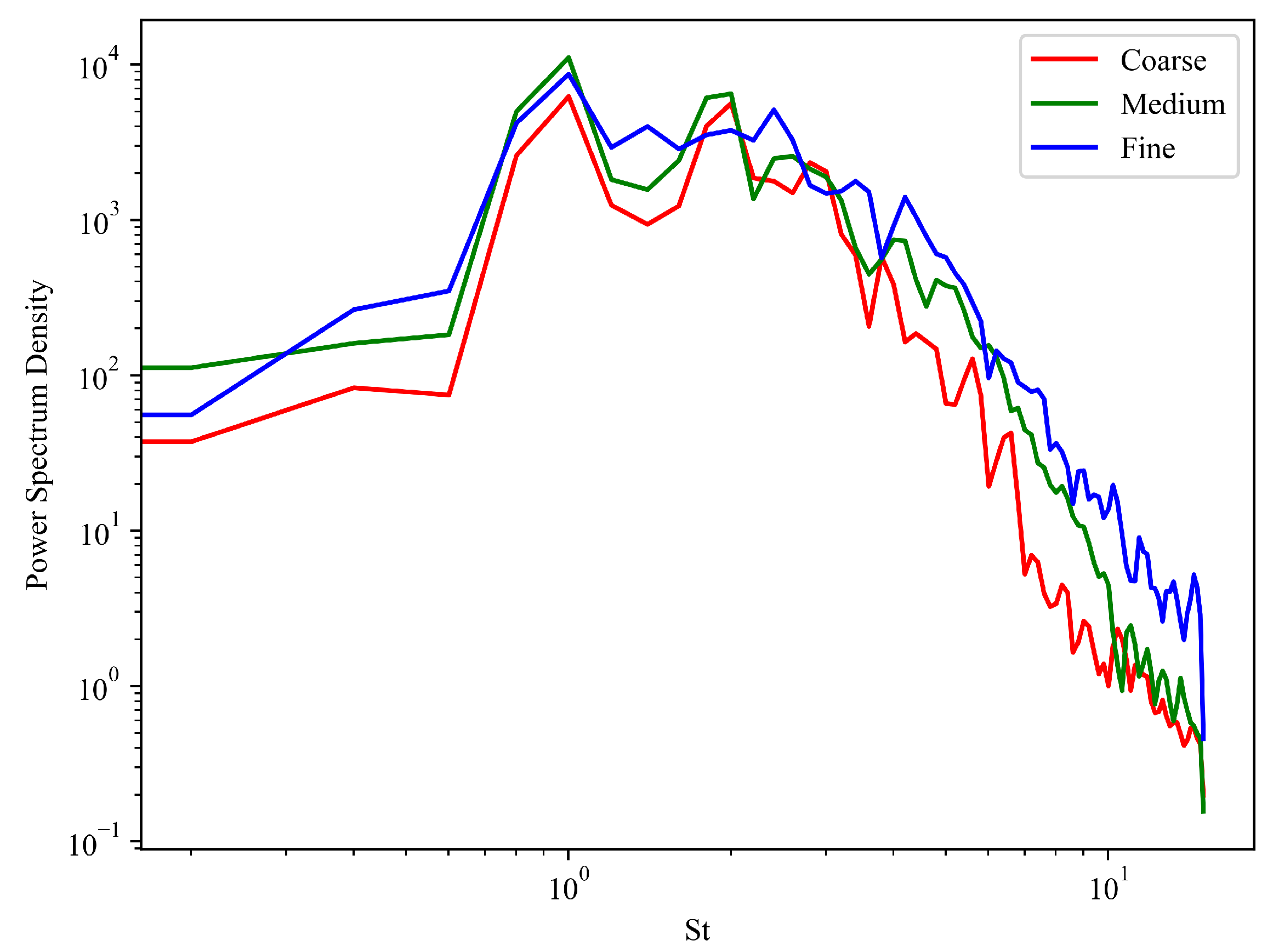
In this work, the initial flow and its quasi-steady structures and behaviors of an underexpanded supersonic jet impinging directly on a flat plate at a low separation distance of less than two nozzle diameters were simulated using rhoCentralFoam, a large-eddy simulation solver of the OpenFOAM framework. Three different levels of mesh resolution were evaluated to confirm grid convergence, and the results were verified with experimental schlieren results. Overall, all meshes were determined to be sufficient for bulk flow properties, such as time-averaged centerline Mach number profile and standoff shock location. However, differences in the resolved vortices, especially those along the jet shear layer, were observed among the three meshes and shown to have an effect on the transient flow structures. These discrepancies will in turn affect the shear-layer/tail shock interactions, which will have cascading effects on time-varying behaviors like standoff shock oscillations. To quantify the differences in the unsteady results of the three cases, a power spectrum density analysis was conducted by probing the pressure of a point within the shear layer. Predictably, the energy dissipation was found to be higher for the coarse mesh and to decrease with increasing mesh resolution.

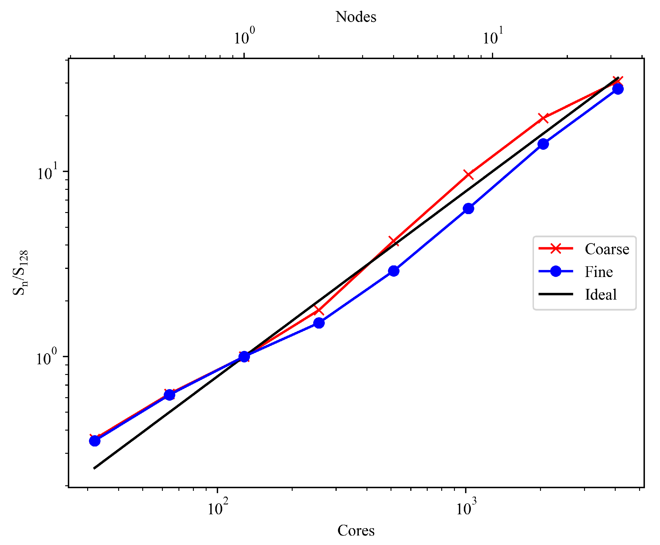
The contrasting observations of the same three meshes being all able to represent the mean SIJ profiles but differing in the unsteady features highlight the fact that the adequacy of a mesh resolution depends on the simulation objectives, whether only net effects are of interest or temporal phenomena have to be properly accounted for. To guide this consideration in the context of rhoCentralFoam, computational scaling analyses were conducted on the three cases, showing that, on current HPC architecture, the solver has good performance in terms of weak scaling. Hence, good estimations on balancing computational resources and compute time for a given mesh resolution can be made. Outstanding strong scaling was also demonstrated, with an approximately linear trend up to 2048 cores (16 nodes) and 4096 cores (32 nodes) for the ∼8.5M and ∼41M cell count cases, respectively.

So far, like previous studies that have considered optimal computational scaling for OpenFOAM simulations [32,45], the discussion has been centered around a “cells-per-core” guideline. However, given the internode communication bottlenecks of OpenFOAM architecture [46,47] and recent significant jumps in cores per node in HPC CPUs, in this work we suggest starting to revise to a “cells-per-node” basis, with particular attention to the interconnect speed and architecture used. This switch implies that an HPC system looking to support a high number of OpenFOAM workloads should not only seek to maximize the core count per compute node, but also ensure the interconnect backbone is sufficient and not a limiting factor. On this note, future studies on the physics of highly transient supersonic impinging jets with low separation distance, which will presumably require large datasets from high-fidelity simulations, can be more effectively conducted.

References

1. Li, S.; Muddle, B.; Jahedi, M.; Soria, J. A numerical investigation of the cold spray process using underexpanded and overexpanded jets. J. Therm. Spray Technol. 2012, 21, 108–120. [Google Scholar] [CrossRef]
2. Alvi, F.S.; Shih, C.; Elavarasan, R.; Garg, G.; Krothapalli, A. Control of supersonic impinging jet flows using supersonic microjets. AIAA J. 2003, 41, 1347–1355. [Google Scholar] [CrossRef]
3. Henderson, B.; Powell, A. Experiments concerning tones produced by an axisymmetric choked jet impinging on flat plates. J. Sound Vib. 1993, 168, 307–326. [Google Scholar] [CrossRef]
4. Krothapalli, A.; Rajkuperan, E.; Alvi, F.; Lourenco, L. Flow field and noise characteristics of a supersonic impinging jet. J. Fluid Mech. 1999, 392, 155–181. [Google Scholar] [CrossRef]
5. Alvi, F.S.; Ladd, J.A.; Bower, W.W. Experimental and computational investigation of supersonic impinging jets. AIAA J. 2002, 40, 599–609. [Google Scholar] [CrossRef]
6. Henderson, B.; Bridges, J.; Wernet, M. An experimental study of the oscillatory flow structure of tone-producing supersonic impinging jets. J. Fluid Mech. 2005, 542, 115–137. [Google Scholar] [CrossRef]
7. Mason-Smith, N.; Edgington-Mitchell, D.; Buchmann, N.A.; Honnery, D.R.; Soria, J. Shock structures and instabilities formed in an underexpanded jet impinging on to cylindrical sections. Shock Waves 2015, 25, 611–622. [Google Scholar] [CrossRef]
8. Sikroria, T.; Sandberg, R.; Ooi, A.; Karami, S.; Soria, J. Investigating shear-layer instabilities in supersonic impinging jets using dual-time particle image velocimetry. AIAA J. 2022, 60, 3749–3759. [Google Scholar] [CrossRef]
9. Munday, D.; Gutmark, E.; Liu, J.; Kailasanath, K. Flow structure and acoustics of supersonic jets from conical convergent-divergent nozzles. Phys. Fluids 2011, 23, 116102. [Google Scholar] [CrossRef]
10. Karami, S.; Edgington-Mitchell, D.; Theofilis, V.; Soria, J. Characteristics of acoustic and hydrodynamic waves in under-expanded supersonic impinging jets. J. Fluid Mech. 2020, 905, A34. [Google Scholar] [CrossRef]
11. Zang, B.; Vevek, U.S.; New, T.H. Some insights into the screech tone of under-expanded supersonic jets using dynamic mode decomposition. J. Aerosp. Eng. 2021, 34, 04021034. [Google Scholar] [CrossRef]
12. Li, X.; Wu, X.; Liu, L.; Zhang, X.; Hao, P.; He, F. Acoustic resonance mechanism for axisymmetric screech modes of underexpanded jets impinging on an inclined plate. J. Fluid Mech. 2023, 956, A2. [Google Scholar] [CrossRef]
13. Ladd, J.A.; Korakianitis, T. On the assessment of one- and two-equation turbulence models for the computation of impinging jet flowfields. In Proceedings of the 32nd Joint Propulsion Conference and Exhibit, Lake Buena Vista, FL, USA, 1–3 July 1996. AIAA 96-2545. [Google Scholar]
14. Dauptain, A.; Cuenot, B.; Gicquel, L.Y.M. Large eddy simulation of stable supersonic jet impinging on flat plate. AIAA J. 2010, 48, 2325–2338. [Google Scholar] [CrossRef]
15. Chan, L.; Chin, C.; Soria, J.; Ooi, A. Large eddy simulation and Reynolds-averaged Navier–Stokes calculations of supersonic impinging jets at varying nozzle-to-wall distances and impinging angles. Int. J. Heat Fluid Flow 2014, 47, 31–41. [Google Scholar] [CrossRef]
16. Cui, W.; Xu, J.; Wang, B.C.; Zhang, P.; Qin, Q. The initial flow structures and oscillations of an underexpanded impinging jet. Aerosp. Sci. Technol. 2021, 115, 106740. [Google Scholar] [CrossRef]
17. Li, M.; Karami, S.; Sandberg, R.; Soria, J.; Ooi, A. Heat transfer investigation on under-expanded supersonic impinging jets. Int. J. Heat Fluid Flow 2023, 101, 109132. [Google Scholar] [CrossRef]
18. Kumar, B.; Verma, S.K.; Srivastava, S. Mixing characteristics of supersonic jet from bevelled nozzles. Int. J. Heat Technol. 2021, 39, 559–572. [Google Scholar] [CrossRef]
19. Lee, J.-A.; Ha, C.S.; Han, J.W. Effect of supersonic oxygen lance on post-combustion in converter steelmaking process–experiment and analysis with converter simulator. Korean J. Met. Mater. 2023, 61, 514–523. [Google Scholar] [CrossRef]
20. Conahan, J.M. High Reynolds Number Millimeter-Scale Jet Impingement Phenomena. Ph.D. Thesis, Northeastern University, Boston, MA, USA, 2021. [Google Scholar]
21. Srivastava, S.; Sheridan, A.M.; Henneke, M.; Raza, M.S.; Sallam, K.A. The structure of inclined choked gas jet. J. Fluids Eng. 2022, 144, 101301. [Google Scholar] [CrossRef]
22. Uzun, A.; Kumar, R.; Hussaini, M.Y.; Alvi, F.S. Simulation of tonal noise generation by supersonic impinging jets. AIAA J. 2013, 51, 1593–1611. [Google Scholar] [CrossRef]
23. Zang, B.; Vevek, U.S.; New, T.H. OpenFOAM based numerical simulation study of an underexpanded supersonic jet. In Proceedings of the 55th AIAA Aerospace Sciences Meeting, AIAA, Grapevine, TX, USA, 9–13 January 2017. AIAA 2017-0747. [Google Scholar]
24. Jasak, H.; Jemcov, A.; Tuković, Z. OpenFOAM: A C++ library for complex physics simulations. In Proceedings of the International Workshop on Coupled Methods in Numerical Dynamics, Dubrovnik, Croatia, 19–21 September 2007; pp. 1–20. [Google Scholar]
25. Vuorinen, V.; Yu, J.; Tirunagari, S.; Kaario, O.; Larmi, M.; Duwig, C.; Boersma, B.J. Large-eddy simulation of highly underexpanded transient gas jets. Phys. Fluids 2013, 25, 016101. [Google Scholar] [CrossRef]
26. Li, T.; Pan, J.; Kong, F.; Xu, B.; Wang, X. A quasi-direct numerical simulation solver for compressible reacting flows. Comput. Fluids 2020, 213, 104718. [Google Scholar] [CrossRef]
27. Modesti, D.; Pirozzoli, S. A low-dissipative solver for turbulent compressible flows on unstructured meshes, with OpenFOAM implementation. Comput. Fluids 2017, 152, 14–23. [Google Scholar] [CrossRef]
28. OpenCFD Release OpenFOAM®v2112. Available online: https://www.openfoam.com/news/main-news/openfoam-v2112 (accessed on 14 March 2023).
29. Expósito, D.; Rana, Z.A. Computational investigations into heat transfer over a double wedge in hypersonic flows. Aerosp. Sci. Technol. 2019, 92, 839–846. [Google Scholar] [CrossRef]
30. Escarti-Guillem, M.S.; Hoyas, S.; García-Raffi, L.M. Rocket plume URANS simulation using OpenFOAM. Results Eng. 2019, 4, 100056. [Google Scholar] [CrossRef]
31. Prokein, D.; Dittert, C.; Böhrk, H.; von Wolfersdorf, J. Numerical simulation of transpiration cooling experiments in supersonic flow using OpenFOAM. CEAS Space J. 2020, 12, 247–265. [Google Scholar] [CrossRef]
32. Zang, B.; Vevek, U.S.; Lim, H.D.; Wei, X.; New, T.H. An assessment of OpenFOAM solver on RANS simulations of round supersonic free jets. J. Comput. Sci. 2018, 28, 18–31. [Google Scholar] [CrossRef]
33. Wu, J.; Lim, H.D.; Wei, X.; New, T.H.; Cui, Y.D. Flow characterization of supersonic jets issuing from double-beveled nozzles. J. Fluids Eng. 2019, 141, 011202. [Google Scholar] [CrossRef]
34. Lim, H.D.; New, T.H.; Mariani, R.; Cui, Y.D. Effects of bevelled nozzles on standoff shocks in supersonic impinging jets. Aerosp. Sci. Technol. 2019, 94, 105371. [Google Scholar] [CrossRef]
35. Kurganov, A.; Tadmor, E. New high-resolution central schemes for nonlinear conservation laws and convection–diffusion equations. J. Comput. Phys. 2000, 160, 241–282. [Google Scholar] [CrossRef]
36. Marcantoni, L.F.G.; Tamagno, J.P.; Elaskar, S.A. High speed flow simulation using OpenFOAM. Mecá. Comput. 2012, 31, 2939–2959. [Google Scholar]
37. Monaldi, L.; Marcantoni, L.G.; Elaskar, S. OpenFOAM™ simulation of the shock wave reflection in unsteady flow. Symmetry 2022, 14, 2048. [Google Scholar] [CrossRef]
38. Sutherland, W. The viscosity of gases and molecular force. Lond. Edinb. Philos. Mag. J. Sci. 1893, 36, 507–531. [Google Scholar] [CrossRef]
39. Richardson, L.F. Weather Prediction by Numerical Process; Cambridge University Press: Cambridge, UK, 1922. [Google Scholar]
40. Garnier, E.; Adams, N.; Sagaut, P. Large Eddy Simulation for Compressible Flows; Springer: Berlin/Heidelberg, Germany, 2009. [Google Scholar]
41. Kim, J.; Dally, W.J.; Scott, S.; Abts, D. Technology-drive, highly-scalable dragonfly topology. In Proceedings of the 2008 International Symposium on Computer Architecture, Beijing, China, 21–25 June 2008; pp. 77–88. [Google Scholar]
42. Roache, P.J. Perspective: A method for uniform reporting of grid refinement studies. J. Fluids Eng. 1994, 116, 405–413. [Google Scholar] [CrossRef]
43. Procedure for estimation and reporting of uncertainty due to discretization in CFD applications. J. Fluids Eng. 2008, 130, 078001. [CrossRef]
44. Welch, P. The use of fast Fourier transform for the estimation of power spectra: A method based on time averaging over short, modified periodograms. IEEE Trans. Audio Electroacoust. 1967, 15, 70–73. [Google Scholar] [CrossRef]
45. Axtmann, G.; Rist, U. Scalability of OpenFOAM with large eddy simulations and DNS on high-performance systems. In High Performance Computing in Science and Engineering ’16: Transactions of the High Performance Computing Center; Springer: Berlin/Heidelberg, Germany, 2016; pp. 413–424. [Google Scholar]
46. Culpo, M. Current Bottlenecks in the Scalability of OpenFOAM on Massively Parallel Clusters. In Proceedings of the Partnership for Advanced Computing in Europe. 2011. Available online: https://prace-ri.eu/wp-content/uploads/Current_Bottlenecks_in_the_Scalability_of_OpenFOAM_on_Massively_Parallel_Clusters.pdf (accessed on 14 March 2023).
47. Bná, S.; Spisso, I.; Olesen, M.H.; Rossi, G. PETSc4FOAM: A Library to Plug-in PETSc into the OpenFOAM Framework. In Proceedings of the Partnership for Advanced Computing in Europe. 2020. Available online: https://prace-ri.eu/wp-content/uploads/WP294-PETSc4FOAM-A-Library-to-plug-in-PETSc-into-the-OpenFOAM-Framework.pdf (accessed on 14 March 2023).
Figure 3. Illustration of the OH-grid implemented to represent the circular nozzle with a fully structured hexahedral mesh.
Computation 12 00124 g003
Figure 4. Mean centerline Mach number profile of three levels of mesh resolution, where four distinct segments labeled by (i) to (iv) can be identified.
Computation 12 00124 g004
Figure 5. Comparison of instantaneous (top) experimental and (bottom) numerical schlieren images for a similar SIJ configuration, reproduced from experiments carried out in Reference [34], while the simulation result is generated by the medium resolution mesh. D is the nozzle diameter of 12.7 mm .
Computation 12 00124 g005
Figure 6. Comparison at six different timesteps focusing on the difference in the presence of shear-layer vortices between three levels of mesh resolution. The mean quasi-steady standoff shock location, which is equal for all three mesh resolutions, is denoted by the red vertical line. The thick arrows in the leftmost column indicate the direction of shock motions. The solid and dashed boxes denote large-scale resolved vortices and small-scale mesh dependent instabilities, respectively.
Computation 12 00124 g006
Figure 7. Power spectrum density analysis of pressure data from the coarse, medium, and fine meshes probed from [ x , r ] = [ 0.5 D , 0.5 D ] over a duration of 1 ms within the quasi-steady state. Sampling frequency of 1 MHz and Welch fast Fourier transform [44] using a 150-frame Hanning window with 50% overlap were used.
Computation 12 00124 g007
Figure 8. Speedup ratio (relative to 128-core run) with respect to core/node counts for strong scaling analysis of coarse and fine SIJ cases. The ideal performance line indicates a proportional scaling with the amount of computational resources allocated.
Computation 12 00124 g008