Abstract
This paper presents the state-of-the-art techniques employed in aerothermal modeling to respond to the current observatory design challenges, particularly those of the next generation of extremely large telescopes (ELTs), such as the European ELT, the Thirty Meter Telescope International Observatory (TIO), and the Giant Magellan Telescope (GMT). It reviews the various aerothermal simulation techniques, the synergy between modeling outputs and observatory integrating modeling, and recent applications. The suite of aerothermal modeling presented includes thermal network models, Computational Fluid Dynamics (CFD) models, solid thermal and deformation models, and conjugate heat transfer models (concurrent fluid/solid simulations). The aerothermal suite is part of the overall observatory integrated modeling (IM) framework, which also includes optics, dynamics, and controls. The outputs of the IM framework, nominally image quality (IQ) metrics for a specific telescope state, are fed into a stochastic framework in the form of a multidimensional array that covers the range of influencing operational parameters, thus providing a statistical representation of observatory performance. The applications of the framework range from site selection, ground layer characterization, and site development to observatory performance current best estimate and optimization, active thermal control design, structural analysis, and an assortment of cost–performance trade studies. Finally, this paper addresses planned improvements, the development of new ideas, attacking new challenges, and how it all ties to the “Computational Fluid Dynamics Vision 2030” initiative.
1. Introduction
A significant fraction (approximately one-third) of the total image aberration of ground-based optical observatories has aerothermal causes, most of it attributed to thermal seeing (~80%), wind jitter, and thermal deformations of the telescope structure and optics. These aberrations also carry the largest uncertainty due to their random nature. Through the years, various empirical aerodynamic and thermal management design and operating strategies have been developed and implemented. In the last two decades, however, the optimization of the configuration and operation of these tools is performed by modeling the mountain–observatory interaction and the enclosure interior–structure–optics interaction.
In this paper, we present the state-of-the-art techniques employed in aerothermal modeling to address the current observatory design challenges, particularly those of the next generation of ELTs (extremely large telescopes). This also happens to be the acronym of the first one, currently under construction in Chile by the European Southern Observatory (ESO), with a primary mirror diameter of ~39 m [1]. To avoid confusion, it is often called E-ELT (European ELT or ESO ELT). Across the Atlantic, two such projects exist, the Giant Magellan Telescope (GMT) [2] and the Thirty Meter Telescope International Observatory (TIO) [3]. The two telescopes of ~25 m and ~30 m primary mirror diameter and currently planned for the southern and northern hemispheres, respectively, can provide diverse research opportunities and enable pivotal breakthroughs in nearly all areas of astrophysics from our Solar System to the most distant stars and galaxies, from fundamental physics and cosmology to the search for evidence of life on planets around other stars.
Recent aerothermal modeling applications range from site selection, ground layer characterization, and site development to observatory aerothermal design optimization, thermal control design, structural analysis, and an assortment of cost–performance trade studies. A review of the aerothermal model types employed by the TIO and GMT will be presented. These models are extendable to all optical observatories, including solar, and aspects of them even to radio telescopes. The synergy between modeling outputs (such as surface pressures, integrated forces, moments, temperature fields, and heat transfer coefficients) and observatory integrating modeling (IM) will follow. Finally, planned improvements, the development of new ideas, attacking new challenges, and how it all ties to the “Computational Fluid Dynamics Vision 2030” will be visited.
2. Integrated Modeling Synergy
2.1. Performance Metrics and Requirement Validation
The ELT projects established Key Performance Parameters (KPPs) for measuring, tracking, and managing the evolution of expected observatory performance through construction and commissioning.
The general foundation documents start at the Operations Requirements Document (for TIO) or Concept of Operations (for GMT) and the Science Requirements Document (SRD) (all Level 1) which are derived from predetermined science cases. The SRD requirements are then flowed down to the Observatory Requirements Document (ORD; Level 2) which is the project’s response to the SRD and contains technical requirements that establish the baseline for the construction project. Requirements in the ORD are given in engineering units that can be measured and verified during the Assembly, Integration, Verification, and Commissioning (AIVC) phase of the project.
The KPPs are defined in the ORD and are the engineering requirements that would have the most significant impact to science if they were not met. Many of the Level 2 KPPs link to several of the science requirements. Every Level 2 requirement also has an associated performance budget in the Level 3 Observatory Architecture Document (OAD). Figure 1 indicates the current best estimate (CBE) analysis: allocations from the error budgets, including the KPP budgets, are flowed down in engineering units to the Level 4 subsystem requirements documents.
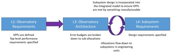
Figure 1.
Cycle of compliance and CBE analysis.
2.2. Integrated Modeling Framework
The integrated model is a single computing framework that combines subsets of specialized models, which are detailed numerical representations of specific properties and functionalities of an ELT [4,5]. It is a composition of several physical models, part of which are also the aerothermal models, and a distributed control system that binds together the sensors and actuators emulated by the different models. An IM instance is a time domain simulation configured with a set of parameters representing a telescope design specification. In addition, models of environmental disturbances provide external boundary conditions to the physical models. Examples of external disturbances are atmosphere and local seeing, wind forces, heat sources, etc. Environmental disturbances are stochastic by nature, and one random occurrence of the disturbances is drawn for each model instance. It follows that optical performance is stochastic too, and the performance of a telescope design is established based on the statistical moments of the optical performance metric (in this case, KPP). Thus, the goal of the IM is to estimate the Level 3 error budget terms and the Level 2 KPPs.
Each simulation of the IM generates an output (KPP value) that is valid for a particular set of disturbance values, called the System State. Each disturbance (or influencing parameter) is discretized with several values that cover its expected range. To span the entire operating envelope, the simulation must be repeated for a different combination of disturbance values. Thus, a multidimensional array of KPP values or look-up tables (LUTs) is generated.
2.3. Stochastic Framework
The observatory system can be considered a stochastic process; its behavior is non-deterministic, in that the system’s subsequent state is determined both by predictable actions and by random elements. Consequently, any metric describing the system performance is a statistical variable. While some performance aspects can be predicted deterministically given a set of inputs, these inputs themselves are usually statistical in nature [6,7].
A wide range of imperfections and external disturbances are truly random in time or through realizations. As an example, the optical effects of thermal deformations of optical elements and their support structure can be deterministically calculated. The inputs to thermal deformation calculations are random environmental and operational parameters. The usual response to this complexity is to intuitively define “representative” and “worst case” scenarios and then to calculate the “mean” and “limiting” performance.
To gain a better insight, we developed a stochastic framework for defining and assessing performance. It is based on site testing data collected by the projects at the sites of the observatories, Maunakea and Las Campanas, as well as on the history of operation sequences of the Gemini North and Magellan observatories [8,9]. The performance of an ELT is expressed for and evaluated against a real observing program carried out in the same environment where it is to be built.
It is not practical for a single, unified model to run through all time frames relevant to an ELT’s performance, from milliseconds to years. Therefore, our approach is to separate physical processes into distinct mathematical models that can be explored somewhat independently. Using the Point Source Sensitivity-Normalized (PSSn) metric [10,11,12] as an example KPP, individual results can be combined to system-level estimates. There are noted exceptions to this approach. In some cases, the time frames of coupled processes overlap sufficiently to justify the development of integrated models. A particular case involves wind, telescope structural dynamics, and control dynamics. For ELTs, this is thoroughly investigated, including the wind buffeting of the primary mirror and the close interaction between the control and structure. Similarly, image jitter due to telescope vibrations is directly addressed in adaptive optics simulations. Over longer time frames, solid (glass and steel) and aerothermal processes are closely coupled. Addressing this coupling requires iterations between the CFD and FEA models or the development of high-resolution conjugate heat transfer models.
The essence of the performance framework is depicted in Figure 2. Group A (red) denotes the available inputs. Group B (blue) is what can be controlled by design and operation. Group C (brown) shows the developed integrated modeling framework output with the pre-calculated aberrations in LUT form (the optics/controls/dynamics/CFD/FEA box is actually the integrated modeling framework). Finally, functions in Group D (green) correspond to mathematical/statistical processing and are in fact the core of the time domain simulation.
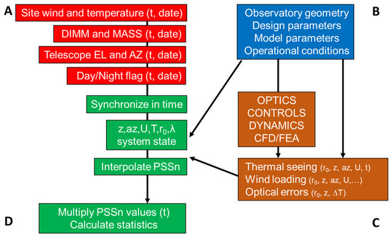
Figure 2.
Stochastic framework flow-chart. (A) environmental inputs, (B) controlled parameters, (C) integrated modeling outputs, (D) data fusion and statistics.
The advantages of this framework are summarized below:
- Allows the statistical representation of errors that are randomized by environmental and operating conditions;
- Allows the statistical representation of errors that depend on previous temporal states of the system;
- Allows the combined representation of errors that are correlated and cannot be assessed independently;
- Allows the combined representation of errors that exhibit disparate time and spatial scales;
- Provides probability distributions of errors to denote the range of expected performance under various seeing conditions, knowledge particularly useful to queue observing;
- Allows the investigation of observatory behavior on different candidate sites;
- Allows the optimization of certain operating strategies, such as venting, daytime thermal treatment, and calibration measurement frequency;
- Unveils the true impact of a particular design decision on the expected observatory performance and subsequent science productivity, enabling cost-effective trade-offs.
3. Aerothermal Modeling Synergy
Thermal management is key to controlling observatory image quality. As tools to minimize thermal effects, ELTs use air conditioning during the day and passive ventilation and heat release control in various forms (subsystem cooling, proper location of heat sources, coatings of desired emissivity) at night. Enclosure surface emissivity and reflectivity are optimized to reduce overheating during the day and overcooling at night.
It is prudent to minimize the difference between the temperature of the telescope (structure and optics) and the average temperature expected at night. Especially for the optics, given their time constant, this is important both for mitigating thermal deformation and mirror seeing. In addition, spatial temperature gradients will be minimized since they are a major contributor to telescope misalignment.
At sunrise, the enclosure will close, and the air trapped inside will start warming up due to the daytime heat release of equipment operating inside the enclosure, solar radiation, and the infiltration of external air. Air Handling Units (AHUs) are connected to chillers/dry coolers in the facilities area. The AHU nozzles supply air to the enclosure interior at several locations, while the returns are located near the observing floor. The goal is to minimize vertical temperature gradients at least up to the height of the telescope and maintain the environment at the expected nighttime temperature by removing all internally generated and externally imposed heat.
At night, radiation loss to the sky through the enclosure opening is balanced by convective heat transfer through the enclosure opening and vents, as well as the heat released into the interior air. The non-uniform spatial distribution of released heat can be particularly detrimental to dome and mirror seeing. Its effect is mitigated by flushing the enclosure with ambient air through the vents. However, at higher wind speeds, enclosure flushing needs to be restricted to limit wind buffeting of the telescope structure and the mirrors. The venting strategy is optimized to balance the thermal seeing and wind buffeting effects. As a baseline, the enclosure vents are expected to be fully open at low external wind speeds, fully closed at high external wind speeds, and partially open at median external wind speeds.
The waste heat removed from the observatory is concentrated into exhaust plumes vented from the farthest point of the facility building which is in the predominantly downwind direction from telescope. During nighttime, the plume’s maximum temperature deviation from ambient is restricted to ensure that any effects on seeing in this direction are negligible.
The models used to simulate the above physical processes are grouped into three main categories based on scope, geometric fidelity, and turnaround time:
- Thermal network models;
- CFD models;
- Conjugate heat transfer models.
Well-known commercial off-the-shelf general-purpose software suites are employed to develop the modeling tools. STAR-CCM+ (2210 or later) [13] is employed to develop three-dimensional representative observatory and subsystem models, while one-dimensional thermal network models, performance frameworks, and post-processors are developed primarily in MATLAB (2020a or later) [14] and Python (3.7 or later).
3.1. Thermal Network Models
These are lumped-mass or one-dimensional transient thermal models. They are computationally inexpensive with short turnaround times. Their main purpose is to estimate surface temperatures, such as for the enclosure skin, as well as other components. These temperatures are used to support the design, to validate requirements, and as boundary conditions to high-fidelity models. Since they are thermal network models, they can accept air as another node so they can also report the mean temperature behavior of a confined volume of air. The true usefulness of these models lies in the fact that the environmental and operational input conditions along with the virtual simulation time span years, thus allowing for the statistical analysis of temperature differentials.
3.2. Computational Fluid Dynamics Models
These are high-fidelity, three-dimensional steady or transient models. They are computationally expensive with long turnaround times. As the name suggests, their purpose is to estimate fluid (air) velocity, temperature, and pressure behavior in space and time, at the ELT sites, around and inside the enclosures, and inside components.
Steady simulations above topography provide ground layer (GL) estimates for site characterization studies. Unsteady daytime-long simulations inside the enclosure provide HVAC performance. Finally, unsteady nighttime simulations provide aerothermal observatory performance, through dome seeing and telescope wind loading. The simulation times for the latter are in the order of minutes.
3.3. Solid and Conjugate Heat Transfer Models
These are three-dimensional transient models. In general, they are computationally inexpensive with short turnaround times, with a few exceptions. Their purpose is not only to estimate component thermal inertia behavior in time but also temperature spatial variability and the resulting deformation. In cases where the effect of a component on a confined volume of air is needed or convective heat transfer variability is important, solid/fluid interaction (conjugate) models are developed. The simulation time for these models is normally a few diurnal cycles.
3.4. Post-Processing Tools
A series of post-processing tools also exist to handle the various intermediate outputs and provide results in the final variable format. Some are incorporated in the software simulation files, and some are standalone.
Figure 3 depicts the current typical ELT aerothermal modeling synergy. The suite consists of a set of thermal network, CFD, and conjugate heat transfer models. It also incorporates a special structural model that has been developed just for thermal deformations. The purpose of these models is not only to provide specific outputs for IQ estimates but also to complement and support each other. Blue corresponds to the high-fidelity CFD models, gold to the conjugate heat transfer, thermal network, and thermal deformation models, green are IQ tools that belong to the IM framework, and yellow are the input/output variables. The CFD models provide heat transfer coefficients to the mirror and telescope structure Finite Element Analysis (FEA) solid thermal models, which in turn provide temperature and heat fluxes to the CFD models as boundary conditions for the telescope and optical surfaces. The network thermal models provide heat fluxes to the CFD models for the enclosure surfaces and other components. They can also provide the FEA models with correct radiation properties. Finally, they can provide fast qualitative information about optimum daytime thermal control strategies to minimize the computationally intensive daytime CFD simulations. The convective heat transfer coefficients needed by the thermal network and FEA models are provided by CFD simulations.

Figure 3.
Aerothermal modeling information flow-chart.
The aerothermal modeling suite can provide a wide range of outputs to validate and/or verify subsystem design requirements. The thermal CFD simulations yield force/moment and temperature fields used, respectively, by the dynamic and thermal seeing blocks, while the thermal FEA simulations yield displacements used directly by the optical block. Thus, it can produce estimates of subsystem aerothermal-related error budget terms and system-level performance budgets.
The available inputs, parameters that can be controlled by design and operation, and pre-calculated aberrations from the IM blocks in multidimensional matrix form (look-up table, LUT) are combined inside the stochastic framework to define the System State in time. Finally, functions corresponding to mathematical/statistical processing produce system-level performance parameters, such as the PSSn.
3.5. Subsystem-Level Inquiry Processing
ELT IM teams have an internal plan for aerothermal model development. The scheduling is tied to system-level reviews, while the specific models are prioritized according to the corresponding error budget term significance. The need for initial estimates of local seeing and telescope wind loading dictated that the first model to be developed and the first subsystem design to be supported and optimized should be the enclosure. A conceptual design-level telescope would be placed inside. Thermal boundary conditions would come from an initial thermal network model that considered large surface areas that directly affect the optical path. The rest of the heat sources would come from the corresponding thermal requirements. This constituted the observatory CFD model. Note here that there exists a nighttime and a daytime version of this model. The model would be updated annually with increasing geometric fidelity. Subsystem models would be developed either to increase thermal boundary condition fidelity for the observatory model, thus increasing performance estimate accuracy, or to support subsystem reviews, as their design matured. This latter process generates what is referred to herein as a subsystem aerothermal inquiry.
The subsystem team contacts the IM team with an inquiry (Figure 4). Typical inquiries can be design trade-off studies (geometric considerations, equipment selection, flow rate and heat dissipation options), input data for survival analysis, and the performance impact of irreversible design choices. These can often be review action items. A meeting or a series of meetings between the teams are held to trace the subsystem requirements directly involved (Level 4) and the corresponding performance requirements (typically Level 3). This is important to define the scope of the action expected by the IM team: what models are required, with what output, and by when. Once the scope is defined, all prerequisites can be identified and required resources estimated.
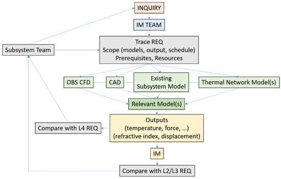
Figure 4.
Representative ELT aerothermal requirement validation process.
Prerequisites include generic inputs (wind speed, telescope orientation, component power/flow rates, etc.), an existing subsystem model, which must be used with different inputs, a CAD model for a new geometry or to update an existing model representation, thermal network models for additional temperature calculations, and system- or subsystem-level heat dissipation budgets. Note that the overwhelming majority of requests to date require information provided by the observatory CFD model.
Often, either the urgency or time scale associated with the inquiry is not compatible with the estimated resources, leading to a de-scoping exercise (minimum amount of effort to produce acceptable answers).
Once all the relevant models and inputs have been identified, the simulations are performed, and outputs are collected. Integrated modeling may or may not be required based on the level of requirements to be validated (or verified). It is common for the first round of results to generate additional inquiries and modifications, along with possibly new model development.
Over the next several sections, the various types and major applications of the aerothermal models will be visited in more detail. To close this section, a summary of the impact aerothermal modeling had on ELT design is presented in Table 1, mostly in timeline order (depending also on the maturity of subsystem design). The summary is not exhaustive. Most models are periodically updated, and their fidelity increases as a result of design maturity and modeling lessons learned. Also, there have been several instantiations of overall performance CBE prior to the development of many of these models. Note, however, that not all observatories followed strictly that order, especially in the site and enclosure selection and design stages.

Table 1.
Aerothermal modeling impact on ELTs.
4. Thermal Network Modeling
The stochastic framework is the basis for any thermal network model to statistically cover a wide range of environmental conditions. Even though the main variable of interest is the ambient temperature, wind and telescope pointing variability provide the required diversity in convective heat transfer coefficients and radiative view factors for both external and internal enclosure surfaces, as well as telescope components. Diurnal environmental records are vital inputs for any thermal network model, since due to thermal inertia, component behavior exhibits “memory”; its current thermal state depends on previous thermal states.
The legacy version of this framework incorporated a lumped-mass thermal model for the TIO primary mirror, since mirror seeing could be calculated using a semi-empirical relation [15]. This relation has been since found not to be valid for giant mirrors and all flow patterns inside ELT enclosures and is not used anymore.
The framework has since been coupled with several thermal network models, which will be presented below. The output parameters of this framework that are used as inputs for other models or for design purposes (operating ranges) include the following:
- Ambient temperature drift since last telescope alignment, used by the telescope/mirror thermal deformation models;
- Temperature differential between sunrise and a particular time of night or mean of night, used for enclosure AHU sizing and to determine supply temperature;
- Temperature differential between daytime external ambient and interior temperatures, using the air conditioning model results, used in combination with external wind speed to determine the enclosure infiltration load.
4.1. Enclosure
Proper thermal boundary conditions on the enclosure surfaces are important for correctly capturing the temperature field inside the optical path. In places where the wind speed is low, diffusion and buoyancy dominate, and the temperature gradients on the surfaces transform into plumes that affect the optical path. Also, as the wind moves over the area around the enclosure aperture, the exterior surface temperature introduces a gradient which then passes through the optical path. In order to estimate the correct heat flux on the enclosure surfaces, a model that can take into account the constant movement of the enclosure components, conduction, convection, and, most importantly, radiation was implemented. It incorporates nodes for the enclosure skin, insulation, enclosure structure, and interior air. It can also provide information on temperature temporal gradients for the interstitial space air, observing floor, and even bulk telescope structure. It can estimate the limits on heat dissipation for specific components. Finally, it can estimate the daytime air conditioning power requirement due to solar radiation, infiltration, and interior heat sources.
A full 3D version of this model for the TIO was first presented in 2011, and the current version is included in [16]. The GMT equivalent can be found in [17].
The impact is as follows:
- Provides Cumulative Distribution Functions of component temperatures and fluxes: exterior skin, enclosure structure, interior insulation, observing floor, enclosure interior air, and interstitial space air;
- Requirements validation: exterior paint and insulation emissivity;
- Provides maximum expected temperature in interstitial space;
- Provides heat dissipation statistics through insulation and observatory floor;
- Provides input boundary conditions to observatory performance CFD simulations.
4.2. Optics
Even though 3D solid thermal models also exist for certain optical components, it is often useful to develop fast lumped-mass counterparts (ex. [18]). The main goal of these models is the requirement verification of allowed residual dissipation after cooling (if required) coupled with the statistical representation of compliance to a surface temperature requirement (typically for thermal seeing purposes).
The impact is as follows:
- Provides glass temperature differential from ambient under various environmental conditions;
- Validation/modification of thermal specifications for primary and secondary mirror systems.
5. Astronomical Site CFD Modeling
5.1. Site Selection
Very early, in 2002, a campaign to identify possible sites for the next generation of a U.S. observatory began. An integral part of this campaign was the use of CFD simulations for validation, site characterization, and short-listing, since equipment could not be deployed on all candidate sites.
Digital Elevation Maps (DEMs) of sites of interest had to be obtained and processed to generate computational domains and meshes. The DEMs covered existing observatory sites, such as Maunakea (Hawaii, USA), Las Campanas (Chile), Paranal/Armazones (Chile), Tololo/Pachon (Chile), San Pedro Martir (Baja peninsula, Mexico), and La Palma (Canary Islands, Spain), and some new ones in the Atacama Desert in Chile (Negro, Honar, Chajnantor, Tolonchar, Quimal) and even in Antarctica (Dome C).
Even though the simulations were initially steady-state and isothermal, focusing on topographically induced mechanical turbulence [19,20], the eventual scope included the resolution and characterization of the GL (optical turbulence), which is more cumbersome to measure experimentally. By 2007, significant progress, including initial model validation efforts, had been achieved on this front as well [21,22,23,24]. A functional dependence on thermal εT and mechanical εM turbulent dissipation was used to estimate the refractive index structure function parameter, Cn2~A εΤ εM−1/3, from steady-state simulations, while the weak scattering theory was used during processing unsteady fields. The CFD simulations produced turbulent kinetic energy and dissipation rates that were subsequently used to calculate the turbulent length scales.
The required inputs include the following:
- Upwind wind and temperature conditions, which, along with topography temperature, result in a realistic GL profile between 7 m and 400 m from the ground. The only variables are wind speed and direction. The ground temperature was chosen to be a calculated quantity rather than input, either by imposing the expected net heat flux or by invoking a gray thermal radiation model with an emissivity of 0.8 and appropriate effective sky temperature. The reference location was that of the corresponding site monitoring system.
- Single reference pressure, reflecting the average site altitude. A user-defined function was used for the corresponding density vertical profile, which resulted in the expected reference density at the average site altitude.
The impact is as follows:
- Primary candidate ELT site selection;
- Risk reduction: validation of GL modeling (comparison with measurements where available);
- Given the appropriate inputs, modeled GL profiles are realistic, while measurement and modeling uncertainties for optical turbulence proved comparable, making the use of thermal modeling an economic and flexible alternative to experiments and in some cases the only option.
5.2. Ground Layer
5.2.1. Maunakea, 13N
The 13N site on Maunakea (HI, USA) is the selected site for the TIO. To that end, a 20 × 13 km2 DEM of Maunakea at 10 m resolution was obtained. The topographic boundary of the computational domain is centered at UTM-5Q [X, Y] coordinates of [241000, 2192500]. Due to the smooth slopes, the height of the computational domain was chosen to be 8000 m for full-scale simulations and 5000 m for simulations confined to 3.5 × 3.0 km2.
During the TIO site selection campaign, temporal records of wind speed, direction, and temperature were collected above the site, along with optical turbulence data. Based on these and the fact that 13N is on the north side, below the summit, steady-state simulations were performed for three wind directions (E, SE, W) under median wind speeds [25].
5.2.2. Las Campanas
Las Campanas Peak (Chile) is the selected site for the GMT. To that end, a 22 × 24 km2 DEM at 20m resolution was fused with a 2 × 2 km2 high-resolution DEM (5 m) of the summit. The topographic boundary of the computational domain is centered at Las Campanas, with UTM-19J [X, Y] coordinates of [336216, 6785453]. The height of the computational domain was chosen to be 5000 m.
Temporal records of wind speed, direction, and temperature, along with turbulent inner-scale and Cn2 values, were collected from the dual-tower environmental monitoring station. Both steady and unsteady CFD simulations were performed for the predominant site conditions, NNE median winds. A procedure was developed to minimize the uncertainty of topographic boundary conditions [26].
5.2.3. La Palma, ORM
The Observatorio del Roque de Los Muchachos (ORM) on the Canary Island of La Palma (Spain) has been selected as the alternate site for the TIO. Several potential locations on the summit needed to be investigated in terms of GL strength. Moreover, the presence of existing observatories necessitated a study of the interaction between these observatories and the TIO. The lack of localized site testing and the nature of the terrain led to the use of CFD simulations combined with a seeing model for GL optical turbulence estimates in 2016 [27].
The location of the ORM on the island of La Palma in combination with rugged terrain and the unavailability of realistic input profiles close to the summit dictated a large computational domain that can encompass almost the entire island with an additional buffer zone at sea level for realistic GL development. At the boundaries of such a domain, velocity and temperature profiles are known with higher certainty. To that effect, a 40 × 40 km2 DEM of the island at 50 m resolution was fused with a 4 × 3 km2 high-resolution DEM (10 m) of the ORM summit. The topographic boundary of the computational domain is centered at the ORM, with UTM-28R [X, Y] coordinates of [217900, 3185029]. The height of the computational domain was chosen to be 7500 m.
Steady-state simulations were performed for four different wind directions (NE, N, W, SW). Two separate studies were conducted. The first one focused on GL comparison between the four candidate sites. Then, for the preferred site based on the results and for two of these wind directions, the presence of nearby observatories such as the GTC and TNG was also considered, to determine mutual interference that could affect the local GL [27]. A more detailed report on the ORM GL variability is given in [28].
The additional impact is as follows:
- Alternate candidate TIO site location selection;
- Evaluation of interaction between the TIO and existing observatories, required by Instituto de Astrofisica de Canarias.
6. Observatory CFD Modeling
Appropriate fidelity CFD models for the observatories have been developed from 3D CAD models of the telescope mount and enclosure. They are used to simulate and analyze the aerothermal environment around the observatories. The developed multimillion-element models account for the major observatory components such as the primary (M1) and secondary (M2) assemblies, the secondary supporting truss-work, other subcomponents of the telescope mount, and the enclosure along with the auxiliary building(s) on the summits.
Upon the conception of the idea of an ELT, the immediate objection that arose was that excessive wind buffeting would render the project unfeasible. The telescope would be too exposed and not stiff enough to perform within the desired specifications. Years of extensive studies had to be performed to resolve the issue [29,30,31,32]. Wind pressure and velocity measurements inside the dome of the still-under-construction Gemini South, wind tunnel studies of generic ELT shapes at Caltech, at the NRC Institute for Aerospace Research in Canada, and in Europe, and CFD simulations and integrated modeling of the structure, controls, and optics finally suggested that an ELT, incorporating the right wind loading mitigation strategies, would not be a futile cause [33]. Armed with additional confidence, legacy studies were performed to converge to acceptable enclosure configurations by simulating conventional dome-shutter, carousel, and Calotte designs and multiple vent and wind mitigation configurations, as well as fixed-base and facility building options. The same techniques developed for the TIO and GMT were also employed for the design optimization of the Vera Rubin Observatory (Large Synoptic Survey Telescope at the time). CFD simulations literally shaped the facilities building architecture, enclosure, light baffles, and camera requirements [34,35,36,37,38].
Across the Atlantic, E-ELT has also performed some nighttime observatory-scale simulations, but they are not tied directly to optical performance, they are focused on velocity levels around the telescope and survival conditions [39].
Detailed reports of the simulation setup can be found in [40,41]. Frequent updates/modifications are necessary due to design evolution and lessons learned from studies, such as the ones reported in [28,42,43,44,45]. The most important ones are summarized in the following:
- The geometries are updated to reflect the latest designs and increased fidelity.
- The heat dissipation budgets are similarly updated, and additional boundaries are created to accommodate the resolved heat sources.
- Advances in meshing methodologies, solver development, and computational power are considered both for simulation setup and output post-processing.
- Upwind domain inputs have been revised to reflect more realistic GL conditions.
- The models retain the relative motion between tessellated parts and the corresponding local coordinates systems to support it. This way, the boundary conditions can be only applied once, and the model templates can be used for multiple orientations and wind speeds. However, for volume meshing, the parts are combined to minimize numerical errors generated at the volume interfaces, to which thermal seeing PSSn calculation is very sensitive. The procedure can still be automated through scripting, if desired.
6.1. Daytime (Air Conditioning)
Daytime CFD simulations were reported in [16,46] between 2010 and 2024 for the TIO and in [47] for the GMT. The simulations performed were selected to demonstrate that the enclosure Heating, Ventilation and Cooling (HVAC) system can perform as expected at least 90% of the time. This is based on the expected daytime heat budget and temperature swing between sunrise temperature and target temperature. The geometry corresponds to a stationary telescope and enclosure at their nominal parking positions.
The impact is as follows:
- Time records of enclosure air temperatures at various heights from the observatory floor and temperature vertical profiles at specified times during the day;
- Validation/verification of HVAC design (max flow rate capacity, split between primary supply and recirculation rates, nozzle location, operating strategy);
- Optimum HVAC nozzle temperature as a function of target temperature to meet performance requirements;
- Provides heat transfer coefficients for convection calculations to component thermal models.
6.2. Nighttime
The current aerothermal performance LUTs consist of results for 3 different telescope zenith angles (0°, 30°, 60°–65°), 5 telescope relative-to-wind azimuth angles (0°, 45°, 90°, 135°, 180°), 5–6 wind speeds (2–3 for open vents, 2–3 for closed), and up to 3 different sets of thermal boundary conditions, corresponding to different parts of the night (nominally ~1 h after sunset, middle of night, and bear sunrise). An effective use of the model involves positioning the mesh at a particular orientation and then running one simulation varying the inlet wind speed between zero and some threshold with open vents. The transition from open to closed vents occurs for an inlet wind speed of ~5–7 m/s. Then, a separate simulation corresponding to wind speeds up to 17–18 m/s with closed vents is performed for that orientation. This way, most of the entire performance wind speed range is covered. The inlet wind speed function is defined so that enough time is spent at the LUT reference wind speeds to eliminate transient effects and accumulate enough time for statistics. This is particularly important for dome seeing due to the longer time scales associated with the diffusion of thermal boundary conditions to the enclosure interior air. Even though this approach has been used to estimate TIO aerothermal performance in the past [45], an alternative will be discussed in a subsequent section.
The additional required inputs are as follows:
- Current thermal boundary conditions on observatory surfaces. The values are grouped into three categories: standard (such as adiabatic, symmetry, etc.), estimated, and assumed. Estimated values are a result of modeling. Assumed values are for components that are either temperature-controlled and have a requirement specification or have insufficient information for accurate thermal modeling. Very few boundaries fall in this category since at least a thermal network model can provide some estimate for most components. For many subsystems, there already exist conjugate heat transfer models that provide surface temperatures. These include optical assemblies, adaptive optics facilities, and some “first light” instruments, with mature enough design. Most boundary conditions are applied as temperature differentials from the ambient reference temperature. In some cases, equilibrium is assumed between convection and radiation, ignoring conduction. These correspond mainly to low-thermal-inertia components, such as the secondary mirror assembly support structure and top end, enclosure and facilities building exterior, and interior surface cladding. Higher thermal inertia component temperatures, such as the enclosure concrete components and telescope lower structure, are given by the corresponding models. Note that proper boundary condition implementation ultimately requires knowledge of the heat balance of the observatory [48].
The outputs include the following:
- Three-dimensional temperature fields inside the optical volume from the M1 vertex until the end of the enclosure boundary layer at a specified temporal sampling rate. These are used as inputs in the thermal seeing post-processor [49,50]. Hence, a byproduct of these simulations is also a time record of Optical Path Difference (OPD) maps. For a historical overview of early thermal seeing modeling, the reader may consult [51,52].
- Time records of pressure maps on optical surfaces. These are used as inputs for wind-induced image blur calculation [53,54]. Pressure maps are also available upon request for any other resolved component.
- Time records of moment components around the telescope coordinate system origin from wind forces on the entire telescope. Forces and moments on isolated resolved telescope components are available upon request. These are used as inputs for image jitter calculation [9,42].
- Convective heat transfer coefficients on selected surfaces for use as inputs in solid and conjugate heat transfer models of components.
Figure 5 presents representative contour snapshots of the refractive index spatial gradient, a measure of optical turbulence, along the normal to the telescope elevation axis plane for the TIO and GMT. Similarly, representative instantaneous OPD maps are shown in Figure 6.
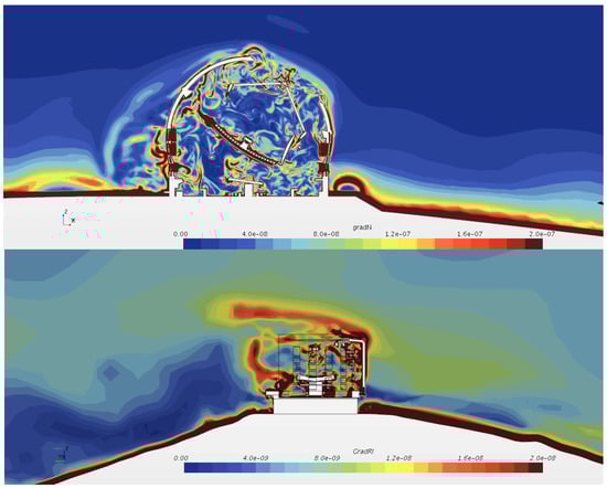
Figure 5.
Representative contour snapshots of the refractive index spatial gradient along the normal to the telescope elevation axis plane: (top) TIO, 30° zenith and 45° azimuth relative to wind, and (bottom) GMT, 0° zenith and 180° azimuth relative to wind. Wind speeds are median (6–7 m/s), and venting configuration is “open”.
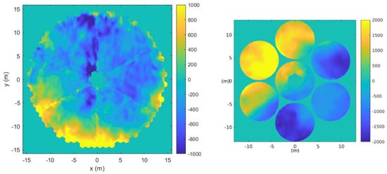
Figure 6.
Representative OPD maps (in nm) for TIO (left) and GMT (right).
The impact is as follows:
- Observatory-wide aerodynamic optimization and enclosure operating strategy development through a trade-off between wind jitter and thermal seeing;
- Observatory performance and error budget terms estimate: thermal seeing, image jitter, and wind-induced image blur;
- Provides thermal seeing sensitivity to heat sources: heat dissipation budget update and design choices;
- Provides metrology system sensitivity to enclosure environment: expected measurement error;
- Provides heat transfer coefficients for convection and component view factors for radiation calculations to component thermal models.
6.3. Daytime (Solar)
It would be remiss not to mention the special category of observatories where the observations occur during the day: solar observatories. These performance estimate techniques have been recently extended to include enclosure and telescope platform optimization and the validation of requirements on heat shields and active thermal control for the European Solar Observatory (EST) [55].
6.4. Validation
By 2010, significant progress, including initial model validation efforts, had been achieved towards resolving and characterizing the GL [21,25]. In 2018, an additional validation effort was presented, using unsteady simulations this time [26]. With the proper knowledge of environmental conditions, current modeling methodologies can produce realistic and useful results. An illustrative example is depicted in Figure 7 for Las Campanas [28]. The GL is compared to that measured at Paranal, ESO’s Very Large Telescope (VLT) site. Paranal is also very close to E-ELT’s site. These profiles are used by both the GMT and E-ELT to train their Ground Layer Adaptive Optics (GLAO) modes of operation. Similar studies have been being performed for Maunakea and the ORM, as mentioned above.
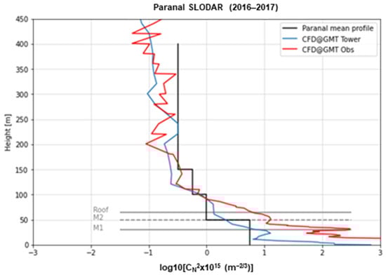
Figure 7.
Cn2 profile at Las Campanas at the monitoring tower and inside the GMT enclosure. The coarse SLODAR-measured profile from the nearby Paranal site is superimposed.
The procedure for nighttime observatory performance simulations with focus on thermal seeing has been validated by studies performed in 2011 and reported in [56,57]. They involved measurements and simulations at two observatories, Keck II and the CFHT (Canada–France–Hawaii Telescope), which share the TIO baseline site and thus computational domain and upwind conditions.
The goal of the studies from the TIO perspective was to validate the modeling procedure necessary to capture local seeing: the numerical method (solver settings and models), required domain size, required observatory geometric fidelity, spatial and temporal resolution, boundary conditions, and representation of heat sources on observatory surfaces.
The Keck observatories were interested in optimizing the use of their active ventilation system to improve performance and minimize operating costs.
The CFHT was interested in the differential performance of a passive ventilation system before deciding to move forward with its approval.
A laser scintillometer was installed at Keck II that provided integrated Cn2 and average optical turbulence inner-scale values on a 63 m path between M1 and M2, along with sonic anemometers at the top-end support ring to capture mechanical turbulence. The active ventilation system was operated at different speeds. An infrared camera provided temperature differentials from ambient for all observatory surfaces. Similar temperatures were collected at the CFHT. A combination of data from CFHT MegaCam delivered IQ; a DIMM installed at the base of the aperture and one installed at the CFHT monitoring tower provided estimates of the apparent dome seeing.
For all measured subsets, the telescope orientations, external wind speed, direction, and temperature were extracted from the CFHT tower data and the Maunakea Weather Center. Four distinct orientations were simulated for a long period of time for Keck II and three for the CFHT, with and without passive ventilation. In the case of Keck II, 240 combinations of orientation, external wind speed, and fan speed were sampled.
The Keck II outputs are as follows:
- Refractive index variance along the scintillometer path, integrated Cn2: reasonable agreement with measurements;
- Turbulent energy dissipation rate and inner scale: reasonable agreement with measurements;
- Integral length scale: matched aperture width as expected;
- Matched behavior of Cn2 vs. external wind speed;
- Matched behavior of Cn2 vs. fan speed;
- Identified optimal fan speed; half of what Keck was previously using.
The CFHT outputs are as follows:
- Point Spread Function (PSF) of dome seeing along optical path, PSF Full Width Half Maximum (FWHM): reasonable agreement with measurements;
- Significant reduction in dome seeing FWHM with passive ventilation: at least 25% without including surface temperature differential improvement (it proved to be closer to 50%).
The impact is as follows:
- Risk reduction: validation of dome seeing modeling;
- Optimal Keck fan speed selection: operational cost reduction;
- Support of recommendation to ventilate the CFHT dome: differential IQ improvement;
- Overall comment as in the case of site CFD: modeling and measured uncertainties were comparable.
As a first approximation, one could envision the thermal seeing optical volume exhibiting OPD behavior similar to atmospheric with a von Karman spectrum of prescribed outer scale and spectral slope. Simulations have shown that the spectral slope quickly converges to Kolmogorov as resolution increases. The optical path length of current and under design/construction large and extremely large telescopes is several tens of meters, long enough to be considered a “good case” of the GL. Under these conditions, the PSSn could be approximated as follows:
In general, this is a quick and dirty way (with some associated error margin) to convert the FWHM to PSSn for most aberrations for purposes of error budgeting. Note that the PSSn is the integral of the square of the PSF, normalized with that of the reference atmosphere, incorporating information from the PSF wings as well, while the FWHM only refers to the width of the PSF where its strength is half its maximum. Thus, the approximation may not be valid for all types of optical errors. More on this can be found in [11,12,13]. Normally, p = 2 is used (equivalent to a root sum square operation between the error and the reference atmosphere). For the specific thermal seeing term, however, since the thermal seeing optical volume is part of the total seeing column, the value of 5/3 should be used:
With the Keck and CFHT validation campaign and the fact that the authors were involved in systems engineering for three large and extremely large observatories under design, PSF maps for five observatories have become available. Figure 8 summarizes the thermal seeing results (multiple data sets, wind speeds, and orientations per point). The results have been rescaled to correspond to the same reference site atmosphere with Fried parameter r0 = 18cm and a wavelength of 0.5 μm. The simulated PSFs confirm that the above expression for the conversion between the FWHM and PSSn is valid. Moreover, the values for Keck and the CFHT have been independently estimated to be realistic, which renders the predicted performance of the observatories under design also realistic, while the Vera Rubin observatory (LSST) is at its final stages of construction with first light expected in 2025. Note that the nominal total error budget for an ELT in the PSSn is ~0.85.
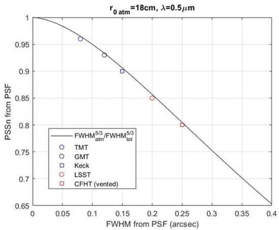
Figure 8.
Observatory simulations: PSSn vs. FWHM.
7. Conjugate Heat Transfer and Solid Thermal Modeling
As explained, the purpose of these types of models is not only to estimate component thermal inertia behavior in time but also temperature spatial variability and the resulting deformation. Thus, the typical required inputs include the following:
- Material and thermal properties of components, including emissivity;
- Ambient temperature profile (either user-defined typical diurnal or subsets of the stochastic framework);
- Active heat loads (component-generated, temporal records if possible);
- Convective heat transfer coefficients (from CFD) for surfaces in contact with air volumes not modeled;
- Thermal resistance between conducting components.
The outputs include the following:
- Time (and space if desired) records of bulk and/or surface temperature differential from ambient for each assembly component;
- Time and space records of node displacements from a reference geometry.
7.1. Mirror Assemblies
The first and most characteristic example of this model category was the TIO Segment Support Assembly (SSA) model. It is a transient model that incorporates conductive, convective, and radiative heat transfer between the segment, the assembly frame, the twelve edge sensors, the three actuators, the corresponding electronics boxes, and the environment.
An earlier version of this model did not incorporate a fluid component. The drawback was that since there was no actual flow pattern away from the segment, convective heat transfer was only treated as a parameter. Since then, the model evolved into its intermediate version, presented in [58]. Here, the fundamental difference is that both the solid and the air temperatures are being solved behind the segment, which eliminates the need for heat transfer coefficient information or “feedback loop simulations” between CFD and FEA. Therefore, the plumes from heat sources, such as actuators and electronics boxes, are accurately represented. For the top segment, surface heat transfer coefficients from the observatory CFD model simulations are used. The correct material properties are used for the segment itself, but for some assembly components that are not 100% solid, density is adjusted so that, given the volume they occupy, the resulting mass is correct. Figure 9 depicts the resolved geometry along with end-of-night surface temperature deviation from ambient, for the final version of the model with increased geometric fidelity.
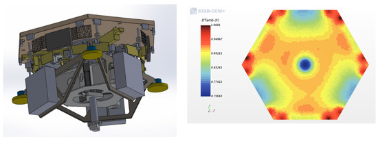
Figure 9.
TIO Segment Support Assembly resolved components (left) and representative front sheet temperature distribution (right).
The GMT M1 mirror segment is made of borosilicate glass with a flat back surface, a parabolic top surface, and mostly hexagonal cores (air pockets) connecting the two sides. The M1 thermal control system (M1TCS) is required to flush the cores with (slightly below) ambient air temperature to track the ambient nighttime air as close as possible. Single-core conjugate heat transfer models were developed for various core heights and nozzle lengths and were simulated for various nozzle flow rates. The goal was to produce a convective heat transfer coefficient (HTC) on the core surfaces that is uniform and comparable to that of the mirror front surface, dictated by the external wind speed, telescope orientation, and venting strategy and obtained from the nighttime observatory CFD simulations.
This way, the deformation of the segment’s front sheet should also be minimal. The air is conditioned by Air Handling Units (AHUs) in the lower plenum of the M1 cell and is guided to the cores by a forest of nozzles. The core flow exits to an upper plenum (UP) volume, separated from the lower plenum (LP) by an insulated steel plate. The upper plenum air can be directed back to the AHUs through intakes on the plate (closed cycle) or exit radially, in which case enclosure air is used by the AHUs (open cycle). The upper plenum can also be sealed from or allowed to communicate with the enclosure air through a gap at the edge of the segment.
Single-core conjugate heat transfer models were developed for various core heights and nozzle lengths and were simulated for various nozzle flow rates, to generate a look-up table of front-sheet HTCs and core flushing efficiency. The HTC on the back sheet, however, depends on the upper plenum flow pattern. So, next, the UP CFD model was developed, resolving all air path inlets and exits, along with the forest of mirror load spreaders (LSs) and core nozzles.
At the same time, it became apparent that, to obtain deformations corresponding to the various design options, a 3D solid model of an entire segment, which takes the expected environment air temperature and surface HTC maps and reports the resulting glass temperature and consequent deformation fields, was required. Note that the on-axis segment varies from the off-axis segments, which means that even though the strategy is identical, all the manual and computational effort is duplicated.
Finally, to confirm that the pressure level and flow pattern created by the AHUs in the lower plenum ensures the desired velocity and temperature uniformity through the nozzles, the LP model was developed, which incorporated all structural components of influence, the AHUs and their ductwork, electrical cabinets and cooling pipework, the actuators and their heat sources, and, of course, the nozzles.
Details of the GMT framework can be found in [18]. Figure 10 shows the M1TCS modeling flow chart with representative model depictions and resulting maps.

Figure 10.
The GMT M1TCS modeling flow chart.
The GMT Adaptive Secondary Mirror System (ASMS) comprises seven deformable 1 m class mirror segments that are designed to function as a single mirror and seven hexapod positioners. Each mirror is deformed by 675 actuators whose dissipated heat is thermally controlled by a cooling plate. The seven crates of the required electronic boards are also actively cooled, while the forty-two hexapod actuators are not. There are also power switch hubs and batteries occupying the top-end space between the support trusses.
A high-resolution solid thermal model of a segment was built, which included the hexapod, frame, electronics crate, cooling plate, reference body, wind skirt, and mirror [59]. The model was attached as the on-axis segment to a reduced version of the mount model (top-end structure, M1 segments, “sky”) in order to properly account for conduction and radiation effects. The remaining six segments and thirty-six actuators were represented as the coarser resolution shapes to be included in the observatory model, and their densities were adjusted in order for their surface temperature to behave similar to the on-axis model over the course of a night.
The need for additional information, such as the refractive index variability at the segment edge sensor locations and the expected differential pressure on the deformable mirror, resulted in modifying the already fine model in order to properly resolve the 100 nm gap between the mirror and the reference body, the actuators themselves as cylinders, and the gaps between them and the reference body as well.
After inspecting the 60 observatory CFD cases in stock, simulations were performed for several wind speeds at the expected impinging angle between the wind and segment, and the differential pressure maps were obtained. Then, the simulations were performed with the coarser resolution segments included in the observatory model, which only provide front pressure maps. A conversion function was formulated so that differential pressure maps from all 60 cases could be generated, which cover the entire range of wind speeds and orientations of interest.
As for the edge sensor environment, 120 s long records of pressure and temperature at 20 Hz were extracted at the sensor locations from the 60 cases, and refractive index spatiotemporal statistics were calculated. These outputs are valuable inputs to the segment co-phasing model.
Figure 11 shows a representative pressure coefficient distribution under median winds on the surfaces of an ASMS segment (half section view).
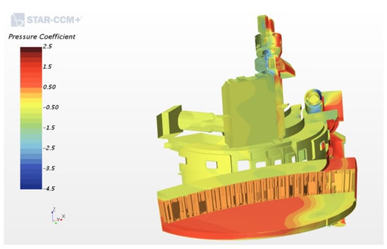
Figure 11.
GMT ASMS model and representative pressure coefficient distribution.
The impact is as follows:
- Validation of thermal requirements on optical assemblies;
- Error budget terms estimate: mirror seeing, segment thermal deformation, and dome seeing;
- Provides realistic expected mirror shapes (thermal, pressure-induced deformation) for actuator correction and phasing.
7.2. Enclosure Systems
The TIO enclosure design consists of a dual-shell geometry, which creates an interstitial space between the external cladding and the interior insulation. Most of the enclosure’s structural thermal mass and heat sources associated with its operation reside in this volume. The required level of insulation might not be achievable everywhere (e.g., vent doors), and seals and gaps might result in undesired infiltration. The telescope azimuth drives reside above the observing floor. In contrast, the GMT enclosure design employs a single-shell geometry, with all the structural thermal mass residing inside the enclosure volume. Most of the enclosure heat sources are behind insulation, and the telescope azimuth drives are below the observing floor.
Transient models have been developed to assess the thermal environment in these interstitial spaces and investigate potential mitigation strategies. The models include all major components and expected heat sources involved, such as the thermal inertia of steel and concrete structures, thermal loads from electrical panels, and interactions with the exterior environment and ground. Particular emphasis is given to the enclosure azimuth corridors, due to the large drive power output and bogie thermal mass in a confined environment with limited and/or expensive ventilation options. The scope is to maintain the temperature below a specified limit given the insulation specifications and the pressure at a level that will deny leaks to the observing chamber either through the seals or through the enclosure vents, when open.
More specifically, the TIO model [16] consists of the following: exterior enclosure cladding, interstitial air in isolated volumes (cap, azimuth corridor, fixed base, vent space), and insulation. Approximately 100 major electrical panels are resolved as blocks. The important heat sources are resolved as solid with internal heat dissipation and the rest as boundaries with prescribed surface heat flux. Even though in the assembly model the enclosure drive heat dissipation is treated as a volumetric source, the magnitude of that source as convective heat transfer is obtained from individual azimuth and cap bogie models, such as the one depicted in Figure 12.

Figure 12.
TIO enclosure azimuth bogie with drive motor: typical nighttime surface temperature distribution.
The GMT model consists of two parts, the Pier Ventilation System (PVS) model (outer and inner fixed base rings, pier, cable wrap, telescope azimuth track, telescope azimuth disk, insulation, interstitial air) and the Mechanical Corridor model (insulation, azimuth track, bogies, break masses, four drive assemblies, and electrical panels). In Figure 13, the PVS model and a steady-state representative air temperature distribution are presented.
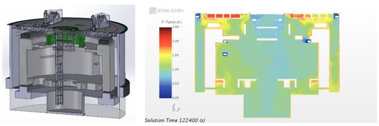
Figure 13.
GMT PVS model (left) and steady-state mid-plane air temperature contours (right).
The impact is as follows:
- Validation of enclosure heat dissipation requirements and insulation performance;
- Design choice: enclosure drives’ and electrical cabinets’ active/passive cooling option and flow rate.
7.3. Telescope Structure
The thermal behavior of an ELT telescope structure (STR) and the STR mounted subsystems depends on the heat load of the system and the thermal properties of component materials and the environment as well as their interactions through convection, conduction, and radiation.
A legacy TIO model from 2010 [60] was based on one-dimensional FEA elements. The resulting displacements were fed into the TIO Merit Function Routine (MFR), which converted them into translations and rotations of the optical surfaces. They, in turn, were multiplied by the TIO optical sensitivity matrix that delivers the corresponding pointing error. Thus, the thermal performance of the structure could be assessed for requirement compliance, and design guidance could be provided. In addition, thermal drift correction strategies and LUTs could be developed.
The latest developed model from 2014 tracks the diurnal temperature variation in the STR and the corresponding deformations [61]. This model is three-dimensional, resolving the thickness of the structural members. It accommodates diurnal simulations and variable elevation angles. It also incorporates all subsystems and components that are thermally coupled to the structure and calculates their temperature as well. Finally, it introduces a “sky” body the size of the aperture, which enables the correct calculation of radiation coupling to the STR. The model consists of the M1 cell, the M3 tower and the lower tube as a single body, the elevation journals, and the upper tube and the spider as a single body. As a later addition, it also incorporates the azimuth structure below the Nasmyth platform, elevation drives and magnets, and hydrostatic pads. Contact interfaces between the distinct bodies are equivalent to welded surfaces. The segment handling and cleaning systems have been omitted, as well as several thin, grated platforms. Additional components, which are only coupled to the structure through radiation, are also included: the M1 control system node boxes, the SSA as a single block of equivalent volume, the M1 as a single body (no segment gaps), the M3 and M2 assemblies, the LGSF, M3, and top-end electronics cabinets, the beam transfer optics duct section above the spider, and the laser launch telescope. The appropriate/desired level of contact thermal resistance between these components and the structure is a parameter. Figure 14 illustrates the end-of-night telescope structure thermal deformation under median expected conditions.
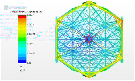
Figure 14.
TIO telescope structure thermal deformation magnitude (m) 12h after sunset.
This model will be revisited in the future, and the study will be updated to reflect the latest design.
A modeling framework of similar fidelity and functionality was recently developed for the GMT mount [62]. The telescope model consists of the M1 segment cells, the elevation journals (C-rings) and hydrostatic pads, the Gregorian Instrument Rotator (GIR), the three secondary support trusses, and the telescope top end with the adaptive secondary mirror. It also incorporates electronics cabinets, actuators, optical baffles, and other equipment that may be thermally coupled with the structure through radiation or conduction. The framework, however, consists of two separate models: one thermal for unsteady temperature calculation and one FEA for steady-state deformation calculation. Three-dimensional snapshot temperature fields from the thermal model, corresponding to various parts of the night, are mapped onto the FEA model to estimate the resulting deformation relative to an initial zero-strain condition, nominally at the time of telescope alignment around sunset. Deformation of the entire structure is available, but the displacements at the hardpoints, the interface between the structure and the optics, are further processed by the GMT optical model to provide the resulting optical misalignment. The goal is to eventually correlate the structure temperature sensor information through a spatial gradient to the optical misalignment and develop an LUT of corrective adjustments as a function of external environmental conditions. Figure 15 depicts the thermal and FEA models.
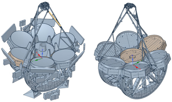
Figure 15.
GMT telescope structure thermal (right) and deformation (left) models.
The impact is as follows:
- Requirement verification: minimum segment gap distance, residual on-sky tracking error, telescope pointing error, maximum actuator stroke, and maximum back focal distance shift;
- Provides realistic expected thermal misalignments for correction strategy testing;
- Provides input boundary conditions to observatory performance CFD simulations.
7.4. Subsystems/Components
7.4.1. Elevation Drives
The modeling of elevation drives started in 2014 with a standalone model to estimate the required cooling flow rate so that the drive surfaces do not exceed a temperature detrimental to dome seeing and the drive coils do not exceed the maximum allowable temperature.
It consists of four major components: the support structure, coils, forcers, and magnets. It is a transient model that incorporates conductive, convective, and radiative heat transfer between the components and the environment. The model was later incorporated into the TIO Telescope Structure Model, as shown in Figure 16.
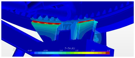
Figure 16.
TIO elevation drive model detail and surface temperature deviation from ambient.
The impact is as follows:
- Validation of EL drives’ cooling flow rate and max coil temperature requirements;
- Provides input boundary conditions to observatory performance CFD simulations.
7.4.2. TIO Laser Guide Star Facility (LGSF)
A model of the LGSF beam transfer optics duct (BTD) was developed in 2013 [63]. It resolved the duct thickness and laser beam transfer mirrors and their support framework for most of the laser beam path that is subject to significant temperature gradients and/or large vertical change. It also resolved the air inside the duct and its thermal interaction with the above components through conjugate heat transfer. The thermal interaction of the laser beam with the optics was also captured. It did not include the path from the eight lasers to the truss pointing array (TPA) or the path inside the laser launch telescope (LLT). The model provided guidance to the LGSF design team and a first estimate of the laser beam stability performance and requirement compliance.
As the telescope structure design evolved through the years, a new optical path was proposed for the LGSF. Both the original and the new optical paths were compared against optical, mechanical, and other telescope performance-related criteria. The optical performance criteria included a first-order analysis of the optical turbulence generated within the ducts. The new proposed path exhibited similar thermal behavior but significantly reduced optical turbulence and was adopted. Design modifications as a result of the study included increasing distances between certain optics and aerodynamic reshaping of the envelopes around the transfer optics. The initial beam jitter estimate was well within the budgeted values.
Between 2021 and 2023, the model was updated to include the laser bench (LB) array, the top-end (TE) assembly, and the LLT [64]. Higher geometric fidelity was also achieved with additional equipment and a support framework. The model was split into five sub-models (LB array, TPA, BTD, TE, LLT), each one feeding the next in terms of flow rate and air temperature. The optical path was split into multiple segments to identify the major contributors to beam jitter and focus error from optics, especially lens, thermal deformation. Beam jitter was calculated as a function of time over the course of the night at both low and high temporal frequency. Additional standalone models of the laser head (LH), standard laser electronics (LE), and top-end electronics (TE.EL) cabinets were developed to verify the expected cooling efficiency and exterior surface temperature. Figure 17 illustrates the modeling flow of information with representative model depictions and resulting optical turbulence contours.

Figure 17.
TIO LGSF modeling flow chart.
The impact is as follows:
- Design modifications to minimize path turbulence and enhance lens cooling;
- Estimates of beam jitter and focus error budget terms.
7.4.3. Electronic/Electrical Cabinets
These are transient models that focus on the shape and volume of a particular component, which typically encompasses an internal heat source. The volume may include multiple parts of different materials, as well as air. Therefore, only the total mass and an average heat capacitance are required to capture their thermal inertia. Their main goal is to provide the distribution of resulting surface temperature and the time it takes the internally dissipated heat to reach the surface given a variable heat source and external environment.
Initially, they were developed as standalone models for a few given components, but recently, they have been routinely included in all assembly models; it is the typical way to treat the average heat source component.
8. Support CFD Modeling
Support CFD models are models of limited scope developed to answer specific design and/or modeling questions. They can be steady or unsteady, and they typically correspond to isolated components.
8.1. TIO Enclosure Aperture Deflectors
The TIO aperture deflectors are a unique feature developed to shield the top end of the telescope from wind as a result of reducing the enclosure diameter to the minimum necessary, but they also act as a seal between the enclosure and the aperture shutter. Figure 18 illustrates the effect of the deflectors on the velocity levels around the top end of the telescope through this early steady-state simulation during the conceptual design phase in 2006. This was equivalent to a ~2.5 m increase in the enclosure diameter. The deflectors have a radius of ~5 m, a chord of ~5 m (tip to hinge), and a projected length normal to the aperture plane of ~3.5 m. When deployed, the angle between the chord and the aperture plane is 45°. During the detailed design phase, the lowest structural mode was estimated approximately at 5 Hz. For both fatigue and survival considerations, the natural vortex shedding frequency and its proximity to the lowest structural modes were evaluated in 2011.

Figure 18.
Impact of the TIO deflector design on velocity levels around the telescope top end (velocity scale normalized with upwind value).
A detailed CFD model of an isolated, single deflector at a 30° angle of attack (the angle expected to determine the maximum shedding frequency) was developed, and unsteady simulations were performed for both median and survival wind conditions [58]. The Strouhal number was calculated, along with the mean and dynamic force components. Under survival conditions, the shedding frequency approaches the first structural mode. The results could be used as inputs to the deflector FEA model to determine the effects of wind loading and investigate design modifications if necessary.
8.2. Spider Beams
The term “spider” refers to the thin multimember truss structure that supports the secondary mirror assembly of a telescope and is present in many existing observatories.
In 2012, an isolated, single spider beam model, at the time 0.25 m × 0.6 m × 20 m, was developed to investigate several modeling assumptions.
The original parametric model used to estimate wind jitter based on steady CFD inputs had assumptions on the beam drag coefficient, the slope of the force spectrum, and the force decorrelation length scale along the beam. The simulations would provide accurate estimates for these assumed values as well as the spatial and temporal resolution required to properly resolve the physics.
Unsteady simulations were performed using various surface resolutions, wind speeds, upwind turbulent intensity, and integral length scale and sampling rate, for flows perpendicular to both the wide and narrow beam sides, as well as angled flow at 30° (combination). The results collected included pressure records on selected locations and integrated force records, as well as mean and RMS drag and lift coefficients.
The results indicated that the parametric model was not valid for local wind speeds above 1 m/s. It also confirmed the assumption that the integrated force spectrum around a solid object has a slope steeper than that of point pressure due to the aerodynamic attenuation effect. The appropriate surface resolution that captures vortex shedding at the expected frequencies was determined and was adopted for the entire TIO telescope structure above the hex ring, the M2 assembly, and the laser launch telescope (LLT). Lower tube resolution was also scaled accordingly. Unsteady simulations would directly provide force records for image jitter estimates going forward. The GMT upper telescope structure is similarly modeled.
8.3. Flow-Induced Pipe Vibration
The phenomenon of flow-induced vibration is well known and potentially problematic for ELTs, especially in AO mode, as the cooling system comprises numerous pipes and bends.
In support of vibration error budgeting, several simple pipe and valve flow models were developed between 2013 and 2021 in a joint TIO-GMT effort to investigate the magnitude of the dynamic force the turbulent flow imposes on the pipe due to friction or separation, as well as its spectrum. A turbulent fully developed straight pipe flow case was first considered and provided the inlet conditions for the remainder of the simulations. These included a 90° bend and an S-shaped pipe, two consecutive 90° bends. Different pipe diameters, ball valve angles, bend radii, and flow rates were also considered.
The results indicated that a single valve could cause larger vibrations than many feet of piping. The piping network should be designed to ensure that valve angles are kept within a threshold limit (<30°). Even though separation frequencies of turbulent flow past a 90° bend can be as high as 200 Hz, the absolute magnitude of the resulting dynamic force is much smaller than the expected pump pressure fluctuations.
8.4. Summit Facilities’ Exhaust
Observatories employ several refrigeration systems used for enclosure daytime air conditioning and the cooling of instrumentation, optics, telescope hydrostatic bearings, etc. The management of the refrigeration cycle heat rejection can be important for IQ. Often, heat rejection occurs at a facility building adjacent to the telescope enclosure. The location and orientation of exhaust vents is selected considering the prevailing wind direction. This approach is based on statistics and might not be very effective for bimodal or multimodal wind environments. A more expensive solution involves building a tunnel to direct the warm air away from the observatory and the optical path. Both the TIO and GMT sites are bimodal, with roughly NE/SW wind orientations.
The chiller of the TIO summit facilities building is therefore located at the NW corner but is expected to discharge warm air in close proximity to the observatory. Under low wind speeds and for certain wind orientations, it is expected that this plume might rise high enough and interfere with the optical path before it has time to diffuse into the air. However, it is expected that the plume can only be a problem under westerly winds and for low elevation angles. Under east winds, the plume dissipates before it crosses the TIO optical path, even under low wind speeds (although the complete absence of wind has never been simulated).
In 2010, a study was performed to assess the plume’s impact on the reference atmospheric seeing. Three CFD steady cases for low (2.5 m/s), median (6.5 m/s), and high wind speeds (10 m/s) from the west (270°) were processed. It is assumed that the results are also valid for west winds between 225° (more common) and 315° (less common). The telescope zenith angle was fixed at 33°. The nominal flow rate of 150,000 CFM resulted in an exhaust velocity of 2.5 m/s and a temperature of ~10.5 K above ambient. The values correspond to an air-cooled unit.
Various optical paths were processed to estimate the equivalent r0 of the first 50 m past the enclosure. Three azimuth (315°, 0°, 45°) and three zenith (65°, 55°, 45°) telescope angles were considered. For each specific telescope orientation, three paths were considered, at X = 0 m and Y = −15 m, Y = 0, and Y = +15 m in the telescope coordinate system. The initial results indicated that considerable impact is detected only for the 65° zenith angle and only for the Y = −15 m path.
As the design evolved, the total power required to be exhausted increased dramatically, and a trade-off between temperature and flow rate was necessary. A new study was performed in 2020 [16] considering various combinations of exhaust temperature differentials and flow rates. Two major changes were implemented for this study. The simulations were unsteady, since advances in GL modeling, as explained in previous sections, allowed for more accurate estimates of the expected FWHM along a path. The exhaust is expected to have louvers that can be optimally arranged to minimize the plume’s effect. Therefore, a 45° down angle was selected. Based on previous experience, the study focused on west 2 m/s winds and the processing of the 315°–45° azimuth sector.
The new study verified that only the lowest part of the optical path is significantly affected at a zenith angle of 65°. It also verified that the plume is not expected to enter the observatory through the vents. An acceptable temperature differential of 15 K above ambient was selected. However, for that temperature, seeing degrades as flow rate increases, which suggests possible exhaust angle and other geometric adjustments. On average, under west low winds and for low elevations, the worst seeing will occur when pointing NE.
Overall, it appears that the plume crosses in some way the telescope optical path when (a) the wind direction is between 225° and 315°, (b) the wind speed is less than a nominal 4.5 m/s, and (c) the telescope azimuth angle is between 300° and 60° and the telescope zenith angle is higher than a nominal 50°. From the stochastic framework, we conclude that this occurs in ~0.4% of the observing time.
The GMT dry coolers are located E-SE of the enclosure, further away and downhill. Their exhaust flow has also been incorporated in the observatory CFD model. Even though they reject heat vertically and at a higher velocity (5 m/s), it is even less likely to affect the optical path. None of the 60 baseline simulations used in the performance assessment suggest any optical path–plume interaction.
The impact is as follows:
- Requirements validation: chiller exhaust temperature differential from ambient, flow rate, orientation, and potential geometric modifications near the facilities’ exhaust area.
8.5. TIO Mechanical Room and Utility Tunnel
In 2015, an extension of the observatory CFD model was developed that included the cable wrap opening on the observing floor and the utility tunnel, as well as the utility and mechanical rooms.
The scope of this study was to investigate the direction of the flow at the cable wrap opening and inside the utility tunnel, the expected temperatures inside the tunnel and utility and mechanical rooms, and the adequacy of the design flow rate inside the tunnel for hazardous gas removal.
Simulations were performed for a configuration that would produce pressure levels inside the enclosure low enough to cause potential flow reversal in the tunnel or locally at the cable wrap opening (median to high wind speed, closed vent, zenith pointing).
Under normal observing conditions, there is only thermal diffusion through the cable wrap that does not really affect the optical path. Under high wind speeds, however, there is flow from the cable wrap opening to the enclosure interior. The tunnel gas removal pipe should not discharge in the utility room but should be connected to the utility room exhaust duct. In order to prevent thermal leakage through the rooms and into the tunnel, the mechanical room exhaust flow rate should be 15% higher than the utility room intake flow rate.
In 2021, the model was revisited and significantly extended to reflect design changes and incorporate higher fidelity [16]. Additions included a bulkhead door that divides the tunnel volume during a fire emergency, the pintle and cable wrap obstructions, and pier and foundation concrete. Additional goals were to assess the impact of closing the bulkhead door on the tunnel flow pattern and the impact of directing the exhausted tunnel air into the mechanical room (as opposed to diverting it directly into the fluid cooling system; we had already determined not to discharge in the utility room).
The study verified that closing the bulkhead door will not have an impact (tunnel flow does not reach the utility room). It also showed that directing the tunnel air into the mechanical room can reduce the exhaust temperature by 2–4 K. Finally, it verified the expected nighttime exhaust temperature level, even though in the first two hours after sunset this level will be significantly higher due to thermal inertia and volume flushing turnaround time (daytime load is much larger).
The impact is as follows:
- Requirements validation: flow sign at cable wrap opening, tunnel fan and utility exhaust flow rates, tunnel gas discharge location, mechanical room exhaust temperature, and temperature environment around equipment.
8.6. Segment Ion Beam Figuring
Several segmented mirror telescopes (e.g., E-ELT, TIO) use Ion Beam Figuring (IBF) to bring the M1 segments to their final figure specifications. During this process, which can last many hours, the segment temperature rises considerably. The bonded joints in the back of the segment can weaken if their temperature exceeds a certain value.
A transient thermal model of the IBF process was developed for the TIO in 2020 with the goal of being able to cheaply test various scanning patterns in order to optimize the process and minimize the temperature rise [65]. Temperature measurements during the IBF experiments for the TIO were used to validate the model. The measurements consisted of a calibration test on a small sample disk (simulated) and three segment runs (two of which were simulated) corresponding to different scan patterns and speeds.
One of the key aspects of the model is the implementation of the Ion Beam flux arriving at the segment surface. This is accomplished by a Gaussian distribution function either on the surface or in a volume of specified thickness. Other important physical phenomena to be considered are diffuse irradiation from the Ion Beam gun as an infrared source, transmissivity through the glass, and potential radiation reflection on surrounding support surfaces. Despite several uncertainties, an initial set of inputs has been identified that could satisfactorily predict the maximum expected temperature at the back of the segment.
8.7. Hexagonal Segment Profilometer
Several existing and future observatories employ segmented primary mirrors consisting of hexagonal segments. In order to verify the final figure specifications of these segments, optical metrology measurements must be conducted. For a particular type of measurement, a laser profilometer, a specific chamber had been proposed by a TIO vendor. In 2012, a model was developed to investigate the relative magnitude of thermal effects such as segment deformation due to non-uniform temperature distribution in the test chamber and variable refractive index along the laser path.
It consists of the following components: laser probe, outer test chamber, glass barriers, segment, support structure, and air inside the test chamber. It is a transient model that incorporates conductive, convective, and radiative heat transfer between the components and the environment. Two configurations of active test chamber ventilation were considered (parallel and counter-flow), results were obtained, and possible error mitigation strategies were suggested.
8.8. Factory Acceptance Tests
More often than not the environment inside a factory or laboratory, where final acceptance tests will be carried out for an observatory component, deviates from that at the actual observatory site. Sometimes a separate set of requirements must be established: if performance during a factory test is X then performance on the mountain should be Y. In such cases a model is used to connect the two. Let us take as an example the “air knife” assembly of the Daniel K. Inouye Solara Telescope (DKIST). It is a key thermal systems component that serves the dual purpose of ventilating the ceiling of the Coude laboratory and as the interface between laboratory and ambient environments using an air curtain. During factory acceptance testing, flow visualization of the air curtain revealed that flow was deflected upwards, suggesting an unexpected pressure gradient, which was confirmed by pressure sensors between the bottom of the assembly and the factory floor. It was hypothesized that large-scale eddies, generated by air knife outflow reversing due to floor proximity, may have induced the increased pressure at the measured locations. The actual CFD model of the assembly in observatory installation configuration suggested that the air knife would meet or exceed all performance requirements [66].
9. CFD Vision 2030
It is evident from the previous sections that the ability to simulate aerothermal flows using CFD has progressed rapidly during the last two decades and has fundamentally changed the aerospace design process. Advanced simulation capabilities not only enable reductions in ground-based (and flight) testing requirements but also provide added physical insight and enable superior designs at a reduced cost and risk. Despite considerable success, the reliable use of CFD has remained confined to a small region of the operating envelope due, partly, to the inability of current methods to accurately and/or efficiently predict turbulent, separated flows. As a relevant example, let us mention the effort that began in 2015 to predict the high-resolution asymptotic value of the PSSn in the context of thermal seeing [43]. Even though an uncertainty quantification study was finally performed with satisfactory results [28] and recent E-ELT efforts for localized effects, without resolving the full observatory, also yield realistic results [67], the status can still be summarized in the following lines: “The estimate of the local thermal seeing as expressed in the PSSn metric does not appear to converge with spatial resolution at the limit of feasible, or rather, reasonable computing power. The extent to which this phenomenon is numerical and to which fine-scale contributions can be parameterized and accounted for is still under investigation. Methodologies have been developed to predict the asymptotic value past the simulation’s target resolution cutoff. However, the error margin within which this might be achieved is probably larger than the desired precision for conducting individual moderate heat source sensitivity analysis. Moreover, the time variability of the metric is also larger than the desired precision”.
Computational scientists are summoned to answer whether CFD has reached its limits or should further research investments make CFD accurate, efficient, and reliable enough to enable future revolutionary gains in aerospace system (in our case observatory) performance and ensure verification by analysis. Under NASA sponsorship, Boeing, Pratt & Whitney, Stanford University, Massachusetts Institute of Technology, University of Wyoming, and the National Center for Supercomputing Applications recently conducted the CFD Vision 2030 Study [68].
The study constitutes a roadmap for the development of enabling technologies such as High-Performance Computing (HPC), physical modeling, algorithms and numerical methods, geometry and mesh generation, knowledge extraction, Multidisciplinary Analysis and Optimization (MDAO) with quantified uncertainties, and experimental testing for computational validation campaigns. A CFD Vision 2030 Integration Committee was established within the American Institute of Aeronautics and Astronautics (AIAA) [69], but its scope of promoting revolutionary advances in computational simulation technologies for the analysis, design, certification, and qualification of aerospace systems is very relevant to ELTs as well. The roadmap consists of various milestones to address and overcome certain challenges with the ultimate goal of simulating a complete operating system within a time window long enough to assess mission success. The simulation realization and post-processing, along with estimating performance parameters and their uncertainties, should be one of many, and the turnaround timescale should be weeks, if not days. In the aerospace community, this means, for example, a maneuvering aircraft with a fully resolved and operating engine(s), as well as critical subsystems such as fuel supply. A database of 1000 simulations will create a real-time multi-fidelity feedback tool during system operation. In the next subsections, we will review how this may translate to the case of a ground-based observatory.
9.1. Geometry and Mesh Generation
The first step in a modeling process is establishing the desired geometric fidelity of the simulation. This of course depends on the physical phenomena involved and the simulation scope (outputs). In the case of trade studies between multiple design options, the geometric differences must be well resolved. Unfortunately, the geometric definition of a component, the digital representation of it (CAD model), and the actual manufactured product are not all the same due to tolerance and translation errors between software formats. This may sometimes have implications for performance predictions. The main current challenge, however, is the incompatibility of CAD models with simulation requirements. There are several reasons for this, the first being the aforementioned tolerance errors. Subsystem components put together to create a complete system model do not always combine to create a closed surface that can be meshed either for air (externally) or solid (internally). Aerothermal simulation requirements might also exclude small features that are not expected to affect the aerothermal environment, but their removal is cumbersome, while leaving gaps and holes that again disrupt surface continuity. Modern software developers, both CAD and simulation, are actively working on implementing automated repair techniques, but dividing the effort between them is an active source of contention… On the simulation side, few software suites are able to “shroud” the geometry, within some tolerance, and eliminate unwanted gaps and features. This technique, however, can significantly alter other important details that affect the flow, and manual user intervention is tedious and time consuming. As a result, both the TIO and GMT currently maintain separate simulation CAD models for subsystems. Generating and updating these models to match design progress has been a labor-intensive task. To accommodate an increasing number of models and configurations, best practices from both systems engineering teams and vendors should be implemented. CAD modelers should understand simulation requirements and create assemblies that can be converted to simulation models with minimal effort, maximizing model interoperability. Simulation modelers should continue to follow repair methodology advances, especially on the surface meshing field.
With a geometry representation in place, the next step is the generation of the computational mesh. There are two main mesh categories, surface/normal-to-surface and volume. The former dictates the accuracy of calculated forces on structures and heat dissipation. The latter is responsible for properly resolving vortices in shear layers and wakes. The aerospace community is actively working towards automatic mesh adaptation in high-velocity-gradient regions, either through re-alignment, morphing, or refinement. Complex geometries or moving parts are resolved with multiple, overlapping meshes (overset) that exchange information through interpolation. Minimizing the interpolation error is another active field of research. At this point, let us define the goal for our operating observatory simulation: the telescope is tracking, then slews to another target at a different orientation and continues tracking, while operating the vents and windscreen (where applicable) under variable wind conditions.
In 2014 [70], an attempt was made to develop an observatory CFD model that would accommodate all configurations, orientations, and modes of operation with a single mesh, based on sliding regions. It had the ability to slew, open, and close the vents and convert to daytime configuration for air conditioning simulations. This, however, was achieved with certain geometric and physical compromises. Vent operation relied on porosity, while parts of the telescope azimuth and elevation structure were removed to accommodate their relative motion. Moreover, it has been proven [71] that uniform hexahedral meshes aligned with the optical volume minimize errors in estimating thermal seeing. Therefore, overset is the only way to go for a multi-target, variable-configuration, transient simulation. Vent operation can be achieved with morphing, since motion is one-dimensional. Mesh adaptation around the enclosure aperture and to the wake might also be needed, especially when the telescope points away from the wind at low elevation angles.
9.2. Physical Modeling, Algorithms, and Numerical Methods
The focus of the decade is the accurate representation of unsteady, turbulent separated flows, a common condition inside an enclosure as well. It has been shown [45] that Reynolds-Averaged Navier–Stokes (RANS) models are not able to resolve optical turbulence and that Detached Eddy Simulations (DES) or Large Eddy Simulations (LES) are needed. Currently, great effort is made toward Wall-Modeled and Wall-Resolved LES. Vortices, such as the ones we observe in Figure 5, are best resolved in conjunction with high-order spatial and temporal discretization schemes. Second-order schemes are being replaced by third-, fourth-, or fifth-order ones. Computational scientists should monitor developments in the implementation of these models in the available software and employ them. ELTs currently employ third-order models.
Efforts are continuing toward the prediction of the high-resolution asymptotic value of the PSSn for thermal seeing. In the case of the TIO, with a nominal OPD resolution of ~16 mm, resolving the optical volume alone requires 10 billion elements. As a result, novel approaches are now considered to characterize local seeing PSF behavior from coarser OPD map spectral analysis [31,47,69]. To this end, the help of validation studies and artificial intelligence (see following sections) will be employed.
9.3. HPC
Significant financial resources are invested annually by industry and government organizations in the purchase of petascale HPC systems and the development of exascale HPC systems, capable of performing 1015 and 1018 Floating Point Operations per Second (FLOPS), respectively. These efforts are also transitioning to quantum and bio-computing. Similarly, significant funds and efforts are spent to allow CFD codes to efficiently utilize the new architectures. There are several reasons that dictate the use of HPC systems for observatory CFD simulations:
- Large volume of simulations. The LUT resolution required to characterize the aerothermal performance of the observatory (zenith and azimuth angles, wind speeds and directions, heat release scenarios) can result in hundreds of simulations and dozens of meshes. These performance LUTs need to be updated every time a major design change occurs and subsets of them on a regular basis to accommodate trade studies; thus, the required turnaround timescale is in months.
- Large computational meshes. Accurate wind jitter and thermal seeing require high enough resolution, resulting in a minimum of several tens of millions of elements. Also, to accurately estimate the net heat transfer on enclosure and telescope surfaces, conjugate heat transfer analysis should be enabled, with the enclosure structure, telescope structure, and other important components to be meshed as well in the same simulation. This will double the required mesh size. Finally, proper GL characterization and interaction with the enclosure requires relatively high-resolution mesh to extend in the first 100 m above the topography.
- Large number of timesteps. Thermal seeing PSSn calculation requires simulations in excess of 10 min of virtual time at a sampling rate of 20 Hz or more, especially if the response of an adaptive secondary mirror is to be properly assessed. Moreover, conjugate heat transfer simulations require much longer integration times, dramatically increasing the number of timesteps, where a high-fidelity solution of the air flow is also desired.
ELT integrated modeling teams are working to automate the mesh generation and simulation setup through scripting, a practice also employed by major aerospace manufacturers. Production CFD runs are deployed on an Amazon Web Services (AWSs) cloud system, a cluster of nodes. The configuration of the AWS cluster is driven by the amount of memory and processors of each node, the processor performance, and the data bandwidth required for inter-node communications. After performing scalability analysis, we can settle on the number of nodes of the specific type of instance that provides the required memory, cores, and network bandwidth. The automated process will configure and create the cluster, upload the simulation file, and launch the CFD run. A sweep of the CFD parameter space that generally requires performing approximately 100 CFD runs could easily lead to the need for a 500-node HPC cluster, if we wished to launch all the runs at once.
Let us examine the example of a GMT AWS CFD simulation [59]. Following the launch of a simulation, a local process is started that synchronizes the data produced locally with a remote S3 repository. Some files, once uploaded on S3, trigger Lambda functions that transform the data in the files into new data products that are compatible with the IM input files. Each CFD simulation generates (currently) ~1 TB of data requiring the local hard drive to be configured with the highest read/write IO throughput available. At the end of each simulation, a post-processing script is executed that extracts and consumes data that are only available once a simulation is completed.
The steps involved in a CFD parameter space sweep are as follows:
- Configure and create the HPC cluster with ParallelCluster (the nodes are requested as Spot instances);
- Upload the CFD configuration files to the cluster;
- Launch the CFD simulations on the cluster;
- For each simulation, start the synchronization process;
- For each completed simulation, post-process the output data;
- For each completed and post-processed simulation, terminate the synchronization process;
- For each terminated simulation, delete the local data.
All these steps used to be performed manually by an operator that is responsible for monitoring and managing the entire simulation cycle. The GMT IM is in the process of replacing them with a streamlined, event-driven operation flow that relies on AWS services to monitor and manage the simulation cycle. As an example, a CFD configuration file is uploaded to an S3 repository that, in turn, will trigger an event that transfers the file to the HPC cluster where the CFD case runs, and associated processes are sequenced and launched automatically, providing significant savings in manual labor.
9.4. Knowledge Extraction
Each HPC simulation generates files of 3D temperature fields for thermal seeing, 2D pressure maps on the optical surfaces for wind blur, and integrated forces on various components at each timestep. In addition, various “screenshots” of variable contours are saved for animation purposes. With the volume of simulations, the mesh size, and the number of timesteps increasing, data manipulation and post-processing becomes a major challenge both for purposes of communications and simulation slow-down. This process also requires automation. Once the simulation is on the way, a synchronization process with a remote AWS repository with enough disk space to receive the output data files of the simulation is required. Additional scripts post-process the simulation data, the data are saved locally, the synchronization process is terminated, and the remote data are deleted.
9.5. Validation
The CFD Vision 2030 called for efforts to develop and execute integrated experimental testing to support a computational validation campaign that will benchmark the new models and methodologies. The astronomical community has the test beds already set: existing observatories. Given the limited body of data regarding dome seeing for ground-based observatories [56,57,72,73], its significant contribution to image degradation, and the modeling limitations already mentioned, it is important to continue validating the CFD methodology and results using data from operating telescopes. There exist current efforts to build dome seeing monitoring instruments [73,74].
Similarly, the estimation of the wind jitter of the telescope structure is based on CFD simulations that have not been fully validated experimentally. One of the largest uncertainties lies in the connection between surface pressure fluctuations and resulting telescope mount torques. Wind tunnel tests with physical models could be conducted to validate the analysis of the forces and torques imparted to the mount by wind buffeting. More specifically, validation is required for dynamic wind loading modeling results for both M1 piston and mount top-end forces, both in terms of predicting differential pressure fluctuations and the relationship between velocity fluctuations, unsteady forces, and the resulting mount torque.
9.6. MDAO
With a volume of CFD simulation results and observatory and wind tunnel measurements, a multi-fidelity database can be created. This extends the current stochastic frameworks to be able to perform uncertainty quantification for the various properties and data sources. It will also enable the observatory to utilize this database as a real-time performance estimator and operation optimizer. This will be particularly useful when quick engineering assessments will need to be made to resolve problems during observatory commissioning.
Several of the error mitigation strategies already defined, such as daytime air conditioning and nighttime ventilation, rely on environmental inputs. Current modeling depends on certain reference upwind conditions, which are moreover coarsely discretized in parameter space. However, the information used by observatory operators will be based on available data from engineering sensors and a site or environmental conditions monitoring system, describing temperature, wind speed, wind direction, atmospheric seeing, etc. These measurements are expected to deviate from the modeling reference conditions, and they could be influenced by summit facilities. As such, an operational plan should be formulated to re-reference the LUTs to these readings. Sensitivity analysis techniques and Artificial Neural Network (ANN) methodologies, using the simulation results at the monitoring locations as training data, can be employed to predict changes in system response to varying parameter inputs in near real time (order of minutes, even seconds). The applicability of this real-time tool will include thermal seeing and wind loading mitigation through vent operation and knowledge of dominant turbulent length scales, telescope pointing error, and thermal misalignment correction strategies based on temperature sensors. Thus, combined with the deterministic optical errors and the current measured atmospheric seeing, a snapshot of the system performance in the delivered IQ metric of choice will be available at any given time. Finally, performance forecasting might even be possible through the coupling of the results to computational boundary conditions which are outputs of an atmospheric mesoscale model or any other weather forecasting service. To the extent that the levels and even temporal behavior of atmospheric seeing, wind speed, and temperature can be predicted for the upcoming night a few hours in advance, delivered IQ scenarios can be generated that can enable queue observing, that is, selecting the order of targets, operating mode (seeing limited or adaptive optics), and instrument throughout the night, so as to optimize the IQ and science output.
The status of observatory aerothermal modeling, the existing challenges, and possible mitigations are summarized in Table 2. As expected, due to the non-profit and purely scientific nature of the observatories, the main challenge is funding. A future concern can also be climate/weather change, since ELTs are expected to operate until the end of the century. Note that smaller support studies are not an issue and are routinely performed.
Table 2.
Observatory modeling status.
10. Concluding Remarks
This paper attempted to provide a summary on the role aerothermal modeling has played in ground-based astronomy over the last two decades and to suggest a possible roadmap for the coming decade.
From GL characterization to enclosure aerodynamic optimization, observatory daytime air conditioning, nighttime heat release control, and subsystem design support, CFD and conjugate heat transfer modeling have become indispensable tools in ELT systems engineering. Extensive system modeling and simulations have been conducted to predict system performance and evaluate against technical budgets (e.g., image quality, heat dissipation) and requirements (e.g., pointing accuracy, environmental constraints). Such performance prediction models support four important systems engineering functions: requirement validation, verification, risk mitigation, and trade-off studies. Simulations have significantly influenced ELT design choices. In the trade space today, perhaps there exist fewer opportunities to modify design than to instead support integration, verification, commissioning, and troubleshooting, as well as optimize performance via operational strategies. Hidden challenges and new opportunities, however, lie abundant.
As the projects continue determined on their path of exploration and discovery, so will the efforts to overcome the new challenges. Using novel techniques and embracing modern technologies, aerothermal modeling will make new discoveries to ensure the success of this groundbreaking engineering endeavor.
Author Contributions
Conceptualization, K.V. and G.A.; methodology, K.V.; software, K.V. and R.C.; validation, K.V.; formal analysis, K.V. and R.C.; investigation, K.V.; resources, K.V. and R.C.; data curation, K.V. and R.C.; writing—original draft preparation, K.V.; writing—review and editing, K.V.; visualization, K.V. and R.C.; supervision, G.A., G.T. and R.C.; project administration, G.A., G.T. and R.C.; funding acquisition, G.A., G.T. and R.C. All authors have read and agreed to the published version of the manuscript.
Funding
This research was funded by TIO, contract number TIO.BUS.CON.24.063 and GMTO, contract number GMT-CON-01543.
Data Availability Statement
The data presented in this study are not readily available because they reside in access-controlled repositories. Some are no longer retrievable. Most of these studies are ongoing and the design not finalized. Requests to access the datasets should be directed to gtrancho@tmt.org and rconan@gmto.org.
Acknowledgments
The TMT International Observatory (TIO) gratefully acknowledges the support of the TIO Members and the Gordon and Betty Moore Foundation. The Members and their respective collaborating institutions are as follows: California Institute of Technology (Caltech); the National Research Council of Canada (NRC-CNRC); the Association of Canadian Universities for Research in Astronomy (ACURA); the Department of Science and Technology, Government of India (DST); the Department of Atomic Energy of India (DAE); the National Institute of Natural Sciences of Japan (NINS); the National Astronomical Observatory of Japan (NAOJ); and the Regents of the University of California (UC). This work was supported as well by the Association of Universities for Research in Astronomy (AURA) and U.S. National Science Foundation (NSF).
This work was supported by the GMTO Corporation, a non-profit organization operated on behalf of an international consortium of universities and institutions: Arizona State University, Astronomy Australia Ltd., the Australian National University, the Carnegie Institution for Science, Harvard University, the Korea Astronomy and Space Science Institute, the São Paulo Research Foundation, the Smithsonian Institution, the University of Texas at Austin, Texas A&M University, the University of Arizona, the University of Chicago, and the Weizmann Institute of Science.
Conflicts of Interest
The authors declare no conflict of interest.
References
- European Extremely Large Telescope. Available online: https://elt.eso.org (accessed on 10 June 2024).
- Giant Magellan Telescope. Available online: https://giantmagellan.org (accessed on 10 June 2024).
- Thirty Meter Telescope International Observatory. Available online: https://www.tmt.org (accessed on 10 June 2024).
- Angeli, G.Z.; Roberts, S.; MacMynowski, D.; Fitzsimmons, J.; Dunn, J.; Vogiatzis, K.; Sheinis, A. Modeling Tools to Estimate the Performance of the Thirty Meter Telescope: An Integrated Approach; SPIE 5497(24); SPIE: Bellingham, WA, USA, 2004. [Google Scholar]
- Conan, R.; Angeli, G.; Sitarski, B.; Dribusch, C.; Fitzpatrick, H.; Romano, H.; Vogiatzis, K.; Das, K. GMTO Approach to Integrated Modeling-Based Systems Engineering; SPIE 11450(26); SPIE: Bellingham, WA, USA, 2020. [Google Scholar]
- Angeli, G.Z.; Vogiatzis, K. Statistical Approach to Systems Engineering for the Thirty Meter Telescope; SPIE 7738(45); SPIE: Bellingham, WA, USA, 2010. [Google Scholar]
- Vogiatzis, K.; Das, K.; Sitarski, B.; Schwartz, D.; Conan, R.; Angeli, G.Z. Using a Stochastic Approach to Estimate the Aerothermal Performance of the Giant Magellan Telescope; AIAA 2019-2319; American Institute of Aeronautics and Astronautics: Reston, VA, USA, 2019. [Google Scholar]
- Vogiatzis, K.; Angeli, G.Z. Monte Carlo Simulation Framework for TMT; SPIE 7017(29); SPIE: Bellingham, WA, USA, 2008. [Google Scholar]
- Sitarski, B.; Vogiatzis, K.; Conan, R.; Angeli, G.Z.; Goodrich, R. Performance Estimates for the Giant Magellan Telescope via Statistical Analysis. In Proceedings of the AO4ELT6, Quebec City, QC, Canada, 9–14 June 2019. [Google Scholar]
- Seo, B.-J.; Angeli, G.Z.; Nelson, J. Analysis of normalized point source sensitivity as a performance metric for large telescopes. J. Appl. Opt. 2009, 48, 5997–6007. [Google Scholar] [CrossRef] [PubMed]
- Angeli, G.Z.; Seo, B.-J.; Nissly, C.; Troy, M. A Convenient Telescope Performance Metric for Imaging through Turbulence; SPIE 8127(4); SPIE: Bellingham, WA, USA, 2011. [Google Scholar]
- Conan, R. PSSn as a Function of Field Aberration and M1 Segment Polishing Residuals; GMT-DOC-01940; GMTO Corporation: Pasadena, CA, USA, 2017. [Google Scholar]
- Siemens Simcenter STAR-CCM+. Available online: https://plm.sw.siemens.com/en-US/simcenter/fluids-thermal-simulation/star-ccm/ (accessed on 10 June 2024).
- Mathworks MATLAB. Available online: https://www.mathworks.com/products/matlab.html (accessed on 10 June 2024).
- Zago, L. The Effect of the Local Atmospheric Environment on Astronomical Observations. Ph.D. Thesis, Ecole Polytechnique Fédérale de Lausanne, Vaud, Switzerland, 1995. Thèse No. 1394. [Google Scholar]
- Vogiatzis, K.; Thompson, H.; Trancho, G. Aerothermal Support for TMT International Observatory Enclosure and Summit Facilities Subsystems; SPIE 13094(27); SPIE: Bellingham, WA, USA, 2024. [Google Scholar]
- Sitarski, B.; Vogiatzis, K. HVAC Sizing Thermal Simulations; GMT-DOC-03957; GMTO Corporation: Pasadena, CA, USA, 2019. [Google Scholar]
- Vogiatzis, K.; Fitzpatrick, H.; Conan, R.; Ranka, T.; Muller, G.; Xin, B.; Ashby, D. GMT Primary Mirror Thermal Control System and Thermal Deformation Modeling Framework; SPIE 13099(102); SPIE: Bellingham, WA, USA, 2024. [Google Scholar]
- Vogiatzis, K.; De Young, D.S. Site Characterization through the Use of Computational Fluid Dynamics. In Proceedings of the 2nd Baeckaskog Workshop on Extremely Large Telescopes, Baeckaskog Castle, Sweden, 9–11 September 2003. SPIE 5382(74). [Google Scholar]
- Vogiatzis, K.; Hiriart, D. Numerical Wind Modeling for the San Pedro Martir Sierra in Baja California. Rev. Mex. Astron. Astrophys. 2004, 40, 81–98. [Google Scholar]
- Els, S.; Vogiatzis, K. TMT Studies on the Influence of Short-Term Changes of Local Thermodynamic Conditions on the Seeing: CFD vs. Observations; SPIE 6267(55); SPIE: Bellingham, WA, USA, 2006. [Google Scholar]
- Els, S.; Vogiatzis, K. Revealing the Onset of Convection in Terrestrial Planet Atmospheres. In Proceedings of the IAU S239 Convention of Astrophysics, Prague, Czech Republic, 21–25 August 2006. [Google Scholar]
- Els, S.; Schöck, M.; Skidmore, W.; Travouillon, T.; Riddle, R.; Vogiatzis, K.; Wang, L.; Bustos, E.; Seguel, J.; Vasquez, J.; et al. Observations of the Turbulent Atmospheric Ground Layer during the Site Testing for the Thirty Meter Telescope (TMT). In Proceedings of the EMS 2007-A-00109, Annual Meeting of the European Meteorological Society and 8th European Conference on Applications of Meteorology, San Lorenzo de El Escorial, Spain, 1–5 October 2007. [Google Scholar]
- Els, S.; Schöck, M.; Skidmore, W.; Travouillon, T.; Riddle, R.; Bustos, E.; Seguel, J.; Vasquez, J.; Vogiatzis, K.; Walker, D.; et al. The Site Testing for the Thirty Meter Telescope and its Potential Role in Developing the Short Term Forecasting of Observing Conditions. Astron. Nachrichten 2007, 328, 7. [Google Scholar]
- Els, S.G.; Vogiatzis, K.; Otarola, A.; Schöck, M.; Travouillon, T.; Riddle, R.L.; Skidmore, W.A. Optical Turbulence above Mountains Seen in 3D; SPIE 7733(58); SPIE: Bellingham, WA, USA, 2010. [Google Scholar]
- Das, K.; Vogiatzis, K.; Angeli, G.Z.; Rosenthal, W.; Bouchez, A.; Goodrich, W. GMT Aerothermal Modeling Validation through Site Measurement; SPIE 10705(2)s; SPIE: Bellingham, WA, USA, 2018. [Google Scholar]
- Vogiatzis, K.; Thompson, H.; Roberts, S.; Dumas, C. Ground Layer Studies for the Alternate TMT Site; SPIE 10705(61); SPIE: Bellingham, WA, USA, 2018. [Google Scholar]
- Vogiatzis, K.; Thompson, H.; Rogers, J.; Trancho, G. On the Relationship between Thermal Seeing and Observatory Design; SPIE 12187(74); SPIE: Bellingham, WA, USA, 2022. [Google Scholar]
- De Young, D.S.; Vogiatzis, K. Numerical Simulations of Flow in Extremely Large Telescope Enclosures. In Proceedings of the SPIE 5382-44, 2nd Baeckaskog Workshop on Extremely Large Telescopes, Baeckaskog Castle, Sweden, 9–11 September 2003. [Google Scholar]
- MacMynowski, D.G.; Angeli, G.Z.; Vogiatzis, K.; Fitzsimmons, J.; Padin, S. Parametric Modeling and Control of Telescope Wind-Induced Vibration; SPIE 5497(26); SPIE: Bellingham, WA, USA, 2004. [Google Scholar]
- Vogiatzis, K.; Segurson, A.; Angeli, G.Z. Estimating the Effect of Wind Loading on Extremely Large Telescope Performance Using Computational Fluid Dynamics; SPIE 5497(30); SPIE: Bellingham, WA, USA, 2004. [Google Scholar]
- MacMynowski, D.G.; Blaurock, C.A.; Angeli, G.Z.; Vogiatzis, K. Modeling Wind-Buffeting of the Thirty Meter Telescope; SPIE 6271(25); SPIE: Bellingham, WA, USA, 2006. [Google Scholar]
- MacMynowski, D.G.; Vogiatzis, K.; Angeli, G.Z.; Fitzsimmons, J.; Nelson, E.J. Wind Loads on Ground-Based Telescopes. Appl. Opt. 2006, 45, 7912–7923. [Google Scholar] [CrossRef]
- Sebag, J.; Vogiatzis, K. LSST Camera Heat Requirements Using CFD and Thermal Seeing Modeling; SPIE 7738(13); SPIE: Bellingham, WA, USA, 2010. [Google Scholar]
- Sebag, J.; Vogiatzis, K.; Barr, J.; Neill, D. LSST Summit Enclosure: Facility Design Optimization Using Aero-Thermal Modeling; SPIE 8449(3); SPIE: Bellingham, WA, USA, 2012. [Google Scholar]
- Cho, M.; Vogiatzis, K.; Sebag, J.; Neill, D. Wind Responses of the LSST Secondary Mirror; SPIE 8449(4); SPIE: Bellingham, WA, USA, 2012. [Google Scholar]
- Sebag, J.; Vogiatzis, K. Estimating Dome Seeing for LSST; SPIE 9150(26); SPIE: Bellingham, WA, USA, 2014. [Google Scholar]
- Vogiatzis, K.; Xin, B.; Claver, C.; Angeli, G.Z.; Selvy, B. Dome Seeing Sensitivity Analysis for LSST; SPIE 10705(3); SPIE: Bellingham, WA, USA, 2018. [Google Scholar]
- Marchiori, G.; Rampini, F.; Mian, S.; Ghedin, L.; Marcuzzi, E.; Bressan, R. ELT Dome and Telescope: Performance Analysis Overview; SPIE 10705(13); SPIE: Bellingham, WA, USA, 2018. [Google Scholar]
- Vogiatzis, K.; MacMartin, D.; Wang, L.; Trancho, G. The TMT International Observatory Aerothermal Performance Estimation Procedure; SPIE 13099(100); SPIE: Bellingham, WA, USA, 2024. [Google Scholar]
- Vogiatzis, K.; Das, K.; Angeli, G.Z.; Bigelow, B.; Burgett, W. Computational Fluid Dynamics Modeling of GMT; SPIE 10705(28); SPIE: Bellingham, WA, USA, 2018. [Google Scholar]
- MacMartin, D.G.; Vogiatzis, K. Unsteady Wind Loads for TMT: Replacing Parametric Models with CFD; SPIE 9150(25); SPIE: Bellingham, WA, USA, 2014. [Google Scholar]
- Vogiatzis, K.; Thompson, H. On the Precision of Aero-Thermal Modeling for TMT; SPIE 9911(40); SPIE: Bellingham, WA, USA, 2016. [Google Scholar]
- Vogiatzis, K. Effects of Meshing, Solver Parameters and Post-Processing on Aero-Optical Image Quality Metric Modeling; AIAA 2018-1502; American Institute of Aeronautics and Astronautics: Reston, VA, USA, 2018. [Google Scholar]
- Das, K.; Vogiatzis, K.; Angeli, G.Z. Assessment of Turbulence Models and Mesh Refinement for Aero-Optical Simulations of Large Ground Based Telescopes; AIAA 2018-4156; American Institute of Aeronautics and Astronautics: Reston, VA, USA, 2018. [Google Scholar]
- Vogiatzis, K. Thermal Modeling Environment for TMT; SPIE 7738(11); SPIE: Bellingham, WA, USA, 2010. [Google Scholar]
- Vogiatzis, K.; Conan, R. Preliminary Evaluation of the GMT HVAC System Using CFD; GMT-DOC-03938; GMTO Corporation: Pasadena, CA, USA, 2019. [Google Scholar]
- Thompson, H.A.; Vogiatzis, K. Heat Balance and Thermal Management of the TMT Observatory; SPIE 9150(83); SPIE: Bellingham, WA, USA, 2014. [Google Scholar]
- Pazder, J.; Vogiatzis, K. Dome and Mirror Seeing Estimates for the Thirty Meter Telescope; SPIE 7017(26); SPIE: Bellingham, WA, USA, 2008. [Google Scholar]
- Conan, R.; van Dam, M.; Vogiatzis, K.; Das, K.; Bouchez, A. Modeling the Giant Magellan Telescope dome seeing using fluid dynamics simulations. In Proceedings of the AO4ELT6, Quebec City, QC, Canada, 9–14 June 2019. [Google Scholar]
- Vogiatzis, K.; Angeli, G.Z. Strategies for Estimating Mirror and Dome Seeing for TMT; SPIE 6271(27); SPIE: Bellingham, WA, USA, 2006. [Google Scholar]
- Vogiatzis, K.; Upton, R. TMT Studies on Thermal Seeing Modeling: Mirror and Dome Seeing Model Validation; SPIE 6271(48); SPIE: Bellingham, WA, USA, 2006. [Google Scholar]
- McMynowski, D.G.; Colavita, M.M.; Skidmore, W.A.; Vogiatzis, K. Primary Mirror Dynamic Disturbance Models for TMT: Vibration and Wind; SPIE 7738(14); SPIE: Bellingham, WA, USA, 2010. [Google Scholar]
- Vogiatzis, K.; McMynowski, D.G. Unsteady Aerodynamic Simulations for TMT Primary Mirror Segment Wind Loading; SPIE 7738(61); SPIE: Bellingham, WA, USA, 2010. [Google Scholar]
- Soler, M.; Vogiatzis, K.; Cozar-Castellano, J.; Bonaque, S.; Bello-Asin, M.; Nunez Cagigal, M.; Baretto Cabrera, M. Local Seeing Analysis for the European Solar Telescope; SPIE 13094(153); SPIE: Bellingham, WA, USA, 2024. [Google Scholar]
- Vogiatzis, K.; Otarola, A.; Skidmore, W.; Travouillon, T.; Angeli, G.Z. Local Thermal Seeing Modeling Validation through Observatory Measurements; SPIE 8449(1); SPIE: Bellingham, WA, USA, 2012. [Google Scholar]
- Salmon, D.; Benedict, T.; Baril, M.; Wang, S.-Y.; Thanjavur, K.; Vogiatzis, K.; Racine, R. A Fluid Dynamic Study of the CFHT Dome Using CFD and Water Tunnel Tests; SPIE 8449(2); SPIE: Bellingham, WA, USA, 2012. [Google Scholar]
- Vogiatzis, K. Aerothermal modeling framework for TMT. In Proceedings of the Integrated Modeling of Complex Optomechanical Systems, Kiruna, Sweden, 15–17 August 2011. SPIE 8336(10). [Google Scholar]
- Vogiatzis, K.; Fitzpatrick, H.; Das, K.; Conan, R.; Angeli, G.; Sitarski, B.; Romano, R.; Dribusch, C.; Walls, B. Aerothermal Modeling for Design Support, Requirement Validation and Performance Assessment of GMT Subsystems; SPIE 12187(22); SPIE: Bellingham, WA, USA, 2022. [Google Scholar]
- Cho, M.; Corredor, A.; Vogiatzis, K.; Angeli, G.Z. Thermal Analysis of the TMT Telescope Structure; SPIE 7738(12); SPIE: Bellingham, WA, USA, 2010. [Google Scholar]
- Vogiatzis, K.; Sadjadpour, A.; Roberts, S. TMT Telescope Structure Thermal Model; SPIE 9150(72); SPIE: Bellingham, WA, USA, 2014. [Google Scholar]
- Fitzpatrick, H.; Conan, R.; Vogiatzis, K.; Das, K.; Dribusch, C. A Computational Framework for the Study of the Diurnal Thermomechanical Behavior of the Giant Magellan Telescope; SPIE 13099(98); SPIE: Bellingham, WA, USA, 2024. [Google Scholar]
- Vogiatzis, K.; Boyer, C.; Wei, K.; Tang, J.; Ellerbroek, B. Aero-Thermal Simulations of the TMT Laser Guide Star Facility; SPIE 9148(243); SPIE: Bellingham, WA, USA, 2014. [Google Scholar]
- Vogiatzis, K.; Wang, L.; Trubey, M.; Irarrazaval, B.; Boyer, C. Aerothermal Modeling of the TMT International Observatory Laser Guide Star Facility; SPIE 13099(101); SPIE: Bellingham, WA, USA, 2024. [Google Scholar]
- Vogiatzis, K. Ion Beam Figuring Modeling; Document TMT.SEN.TEC.20.070; TMT International Observatory: Pasadena, CA, USA, 2020. [Google Scholar]
- McQuillen, I.; Phelps, L. Factory Acceptance Testing and Model Refinement for the Daniel K. Inouye Solar Telescope air Knife Assembly; SPIE 10705(25); SPIE: Bellingham, WA, USA, 2018. [Google Scholar]
- Martins, D.; Holzlohner, R.; Verinaud, C.; Kleinclaus, C. Transient Wavefront Error from Cooled Air Downwind of Telescope Spiders; SPIE 12187(12); SPIE: Bellingham, WA, USA, 2022. [Google Scholar]
- CFD Vision 2030 Study. Available online: http://ntrs.nasa.gov/search.jsp?R=20140003093 (accessed on 10 June 2024).
- AIAA CFD Vision 2030 Integration Committee Website. Available online: https://cfd2030.com (accessed on 10 June 2024).
- Vogiatzis, K. Transient Aero-Thermal Simulations for TMT; SPIE 9150(24); SPIE: Bellingham, WA, USA, 2014. [Google Scholar]
- Vogiatzis, K.; Thompson, H.; Roberts, S. On the Precision of Aero-Thermal Simulations for TMT: Revisited; SPIE 10705(4); SPIE: Bellingham, WA, USA, 2018. [Google Scholar]
- Racine, R.; Salmon, D.; Cowley, D.; Sovka, J. Mirror, dome, and natural seeing at CFHT. Publ. Astron. Soc. Pac. 1991, 103, 1020–1032. [Google Scholar] [CrossRef]
- Bustos, E.; Tokovinin, A. Dome Seeing Monitor and Its Results for the 4m Blanco Telescope; SPIE 10700; SPIE: Bellingham, WA, USA, 2018. [Google Scholar]
- Lai, O.; Withington, K.; Chun, M.R.; Laugier, R. Investigating ground layer and dome turbulence in astronomical observatories using a localized optical turbulence sensor. In Proceedings of the Imaging and Applied Optics Congress, Washington, DC, USA, 22–26 June 2020. [Google Scholar]
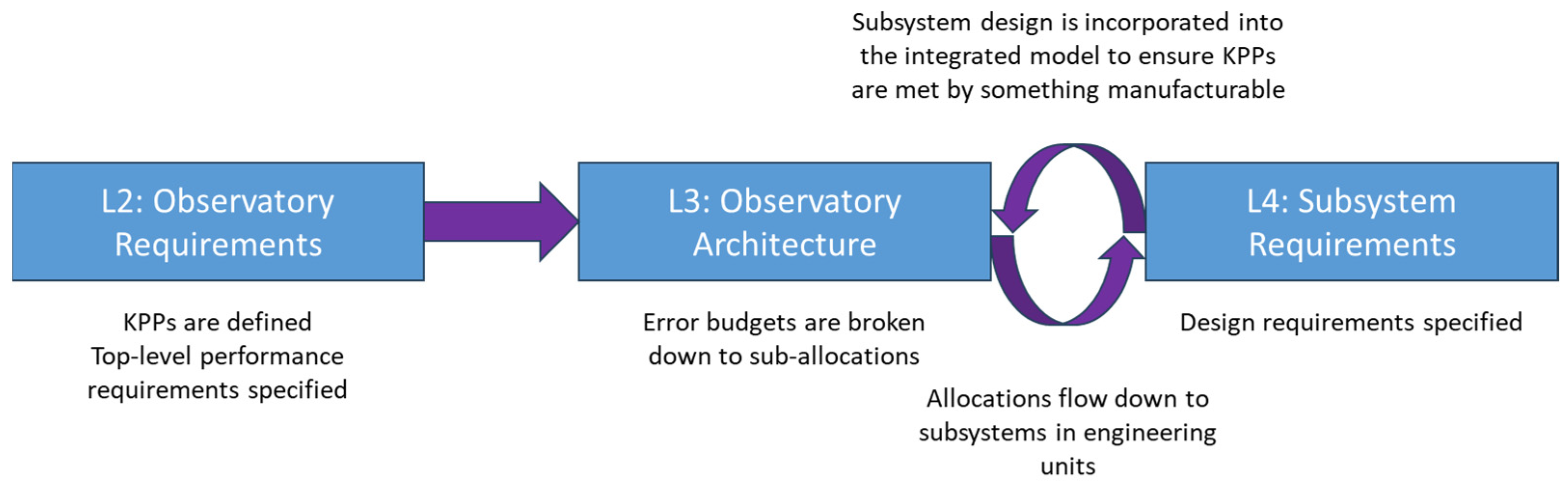
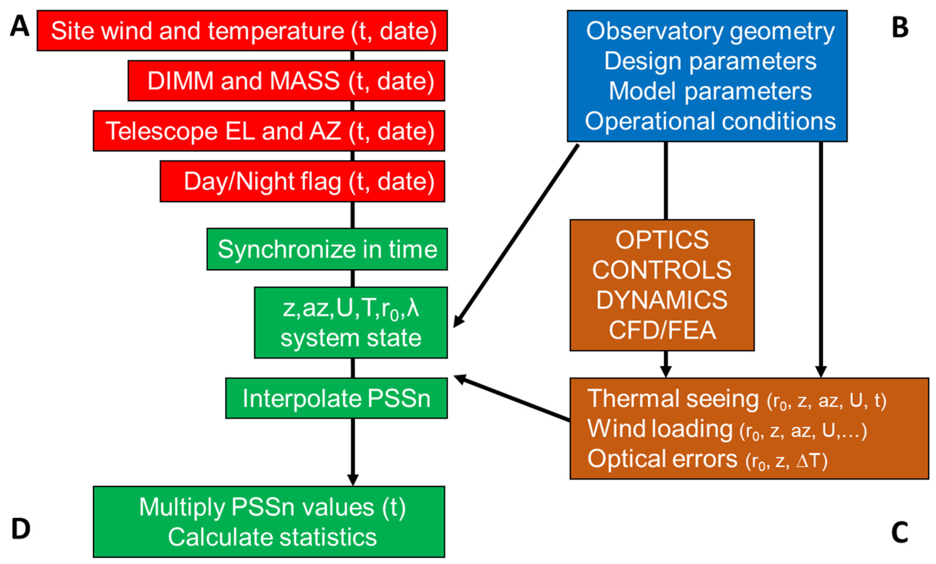
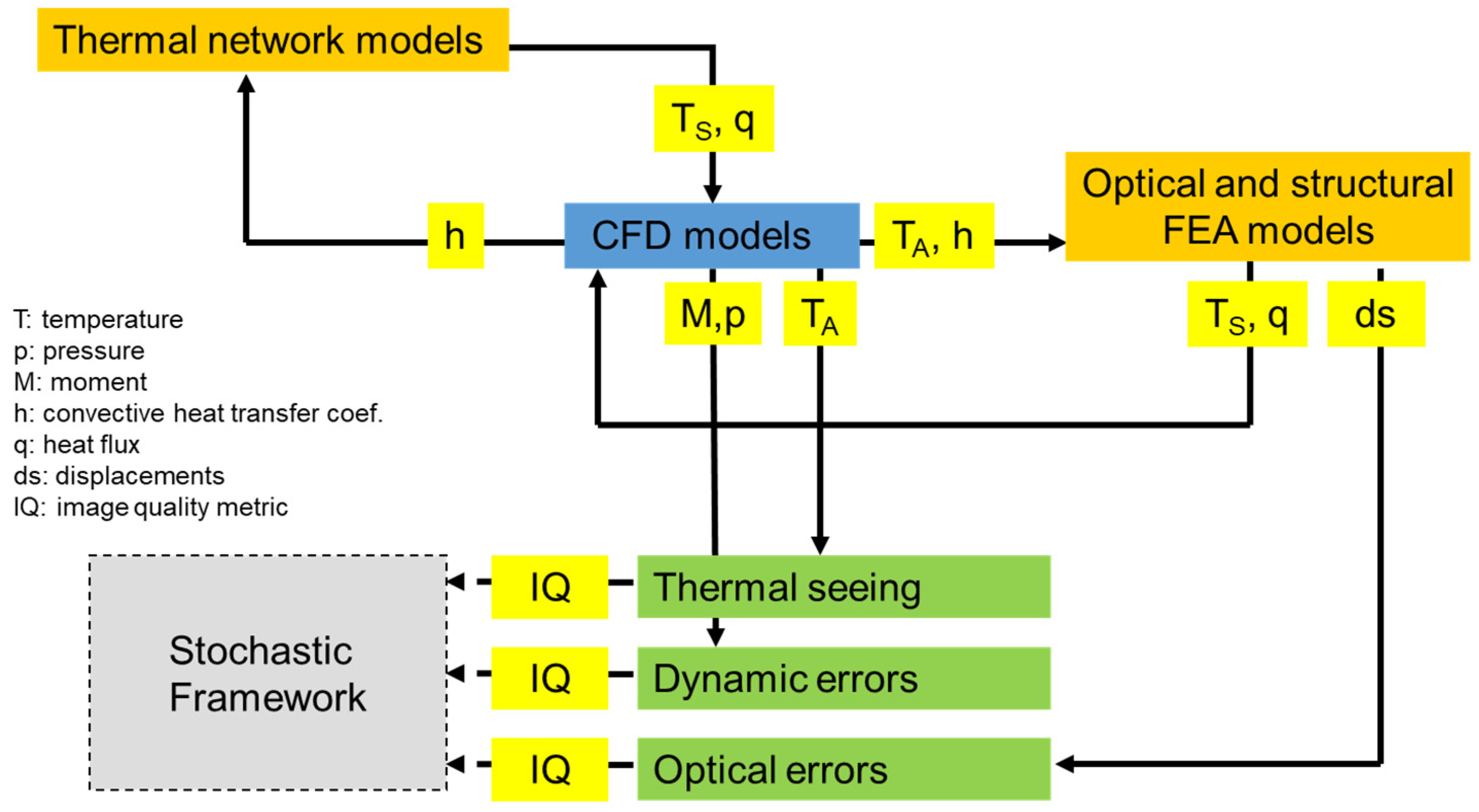


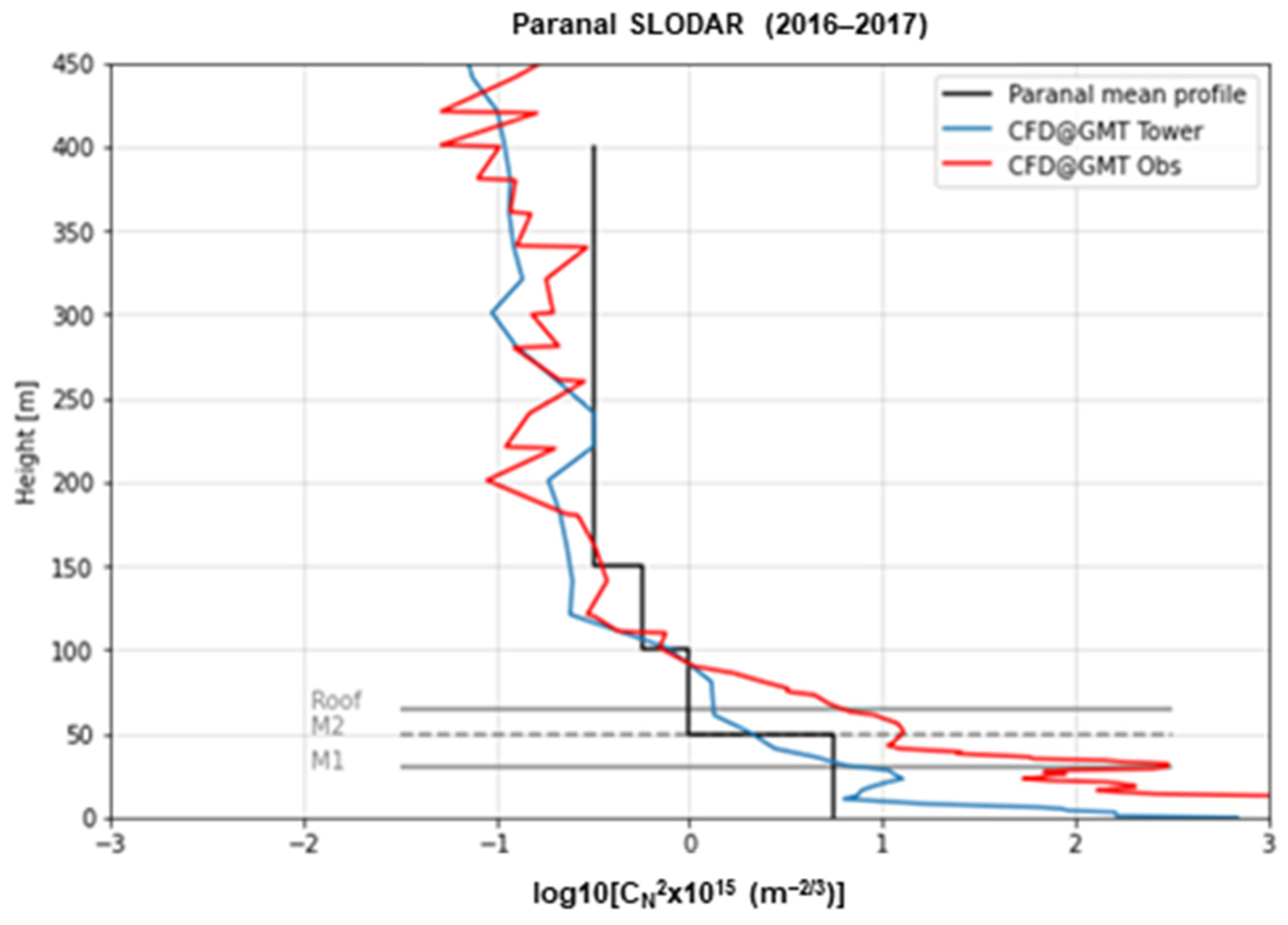
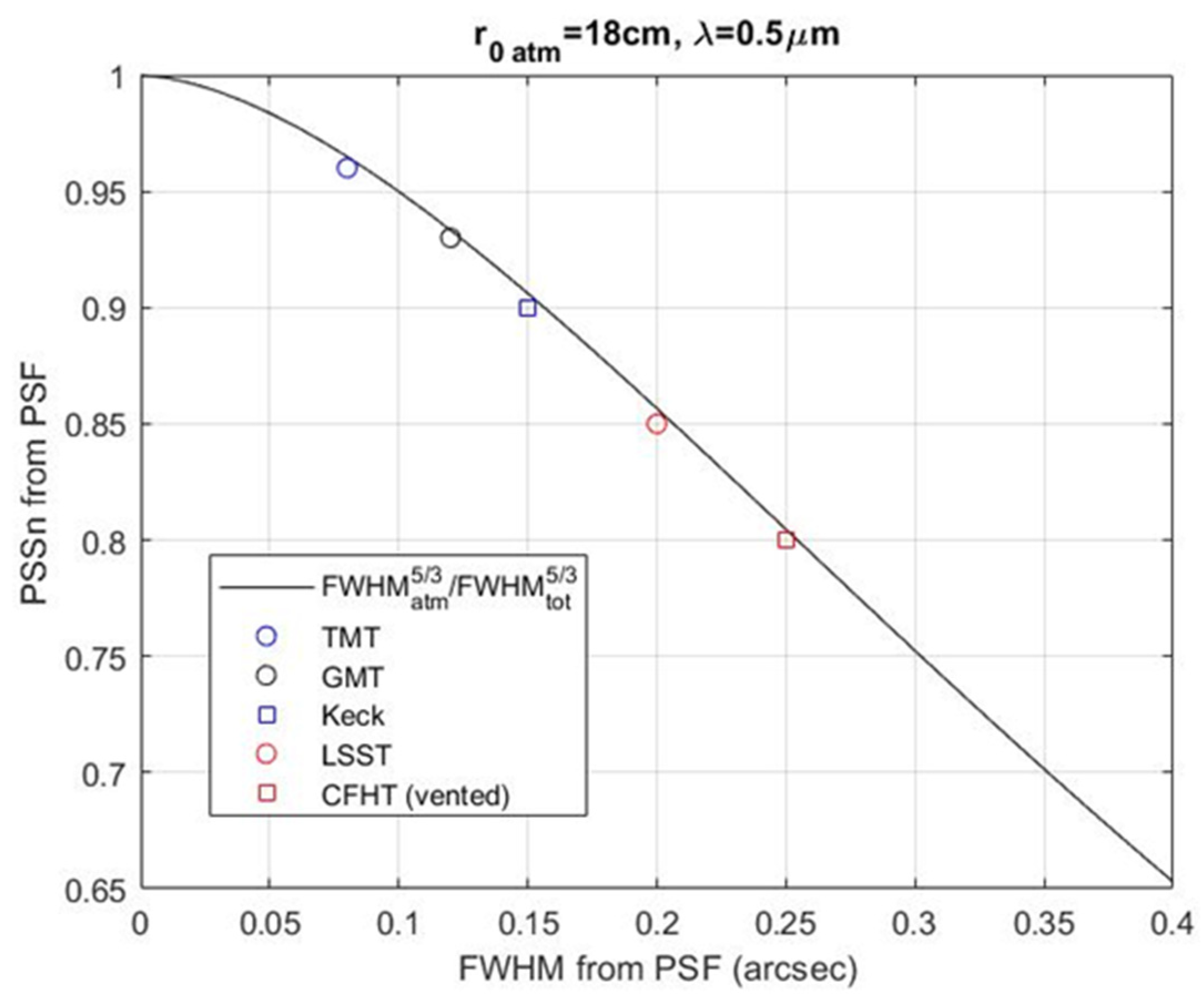

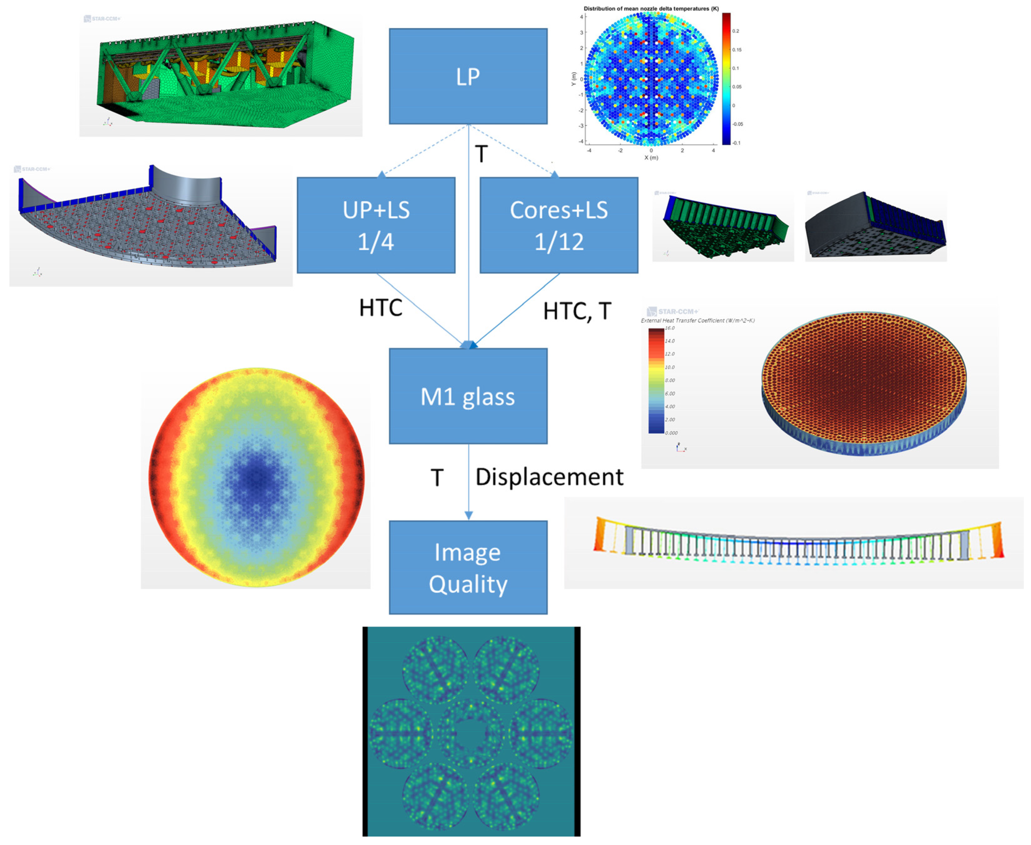

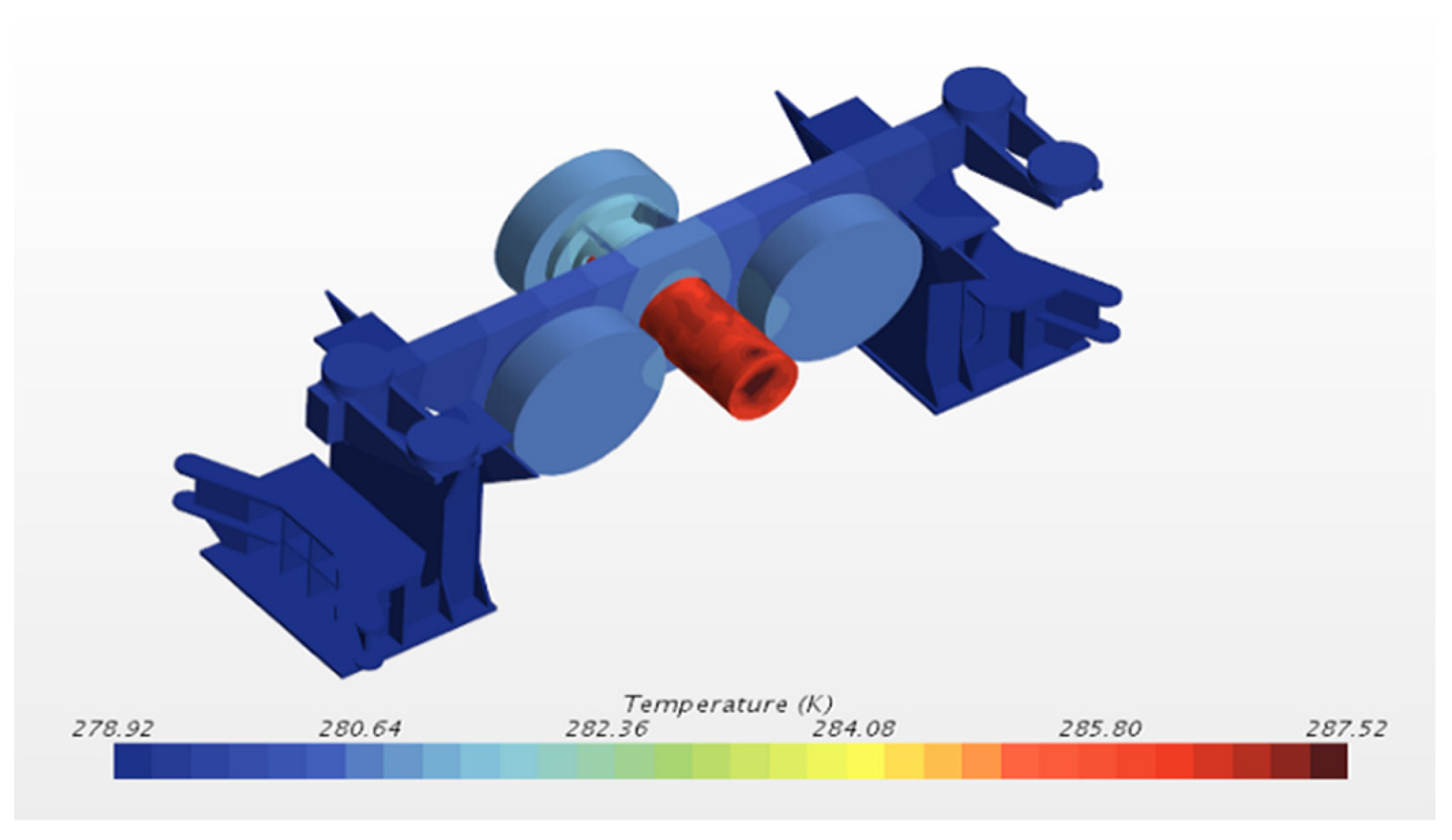
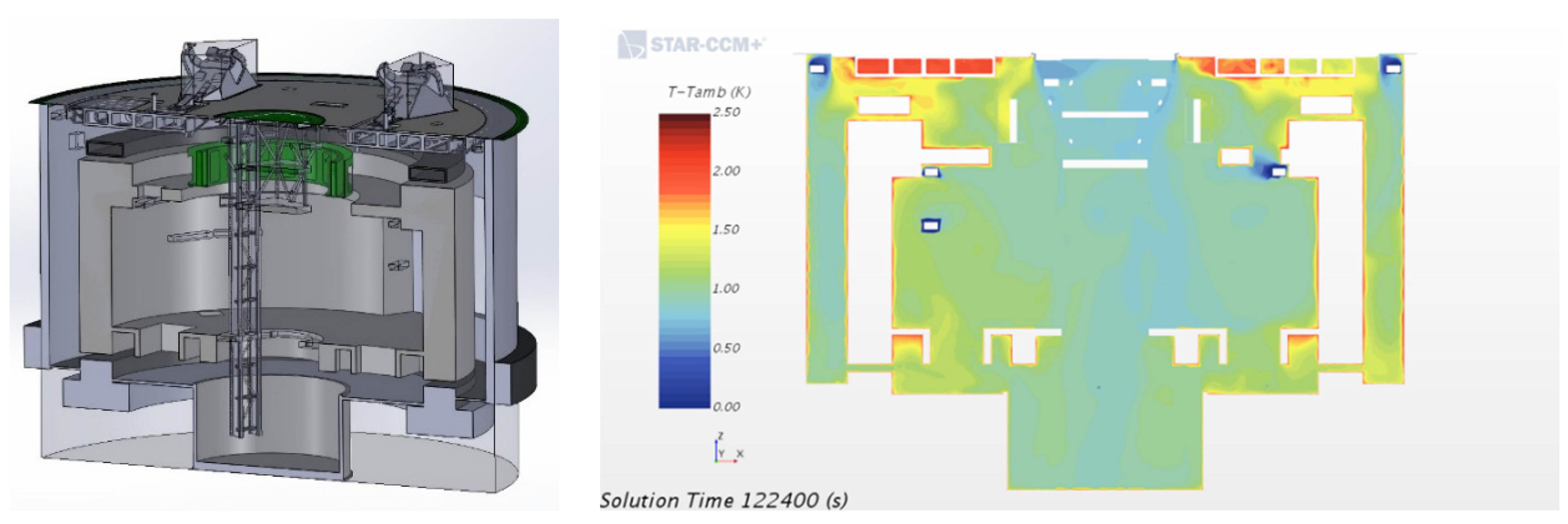

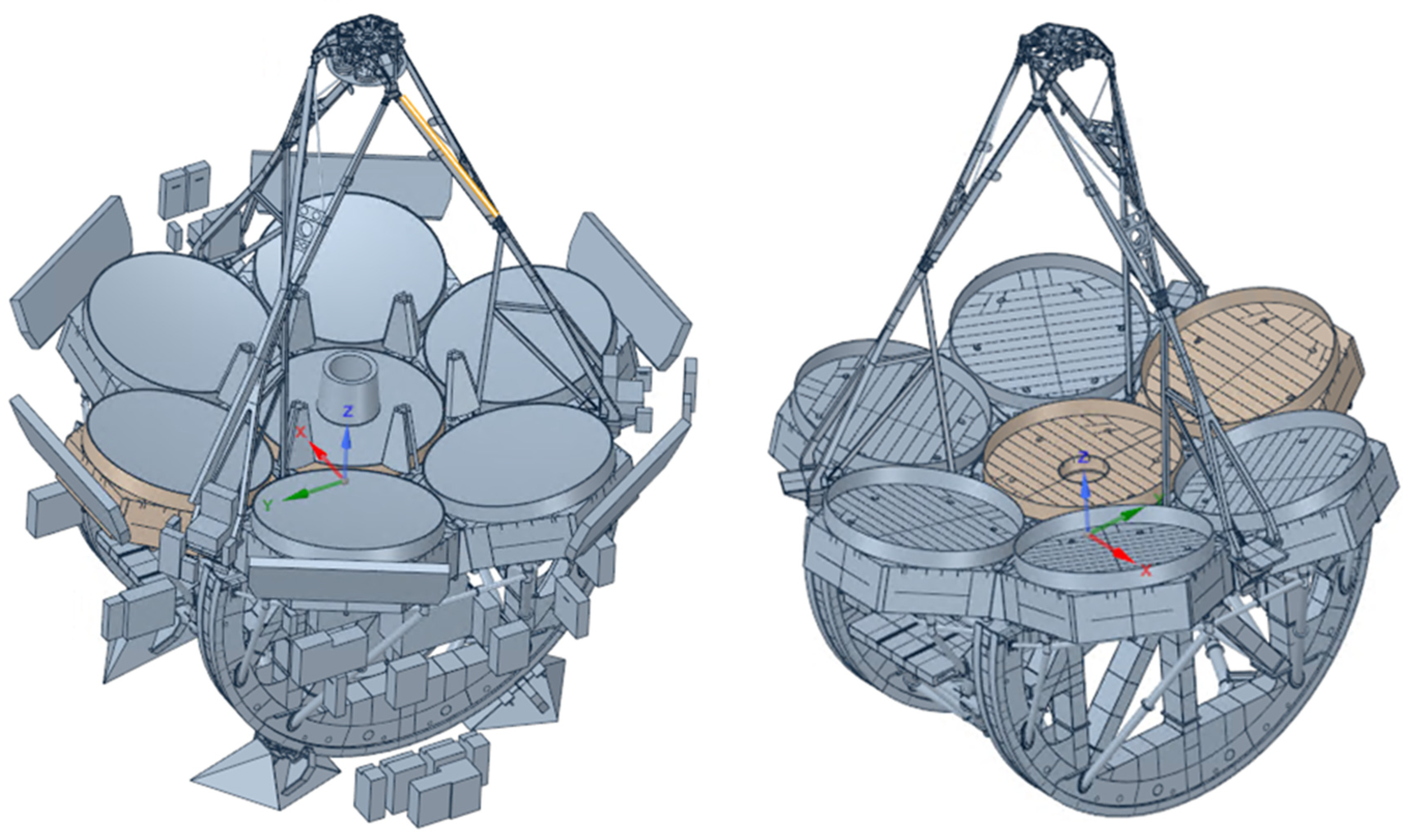

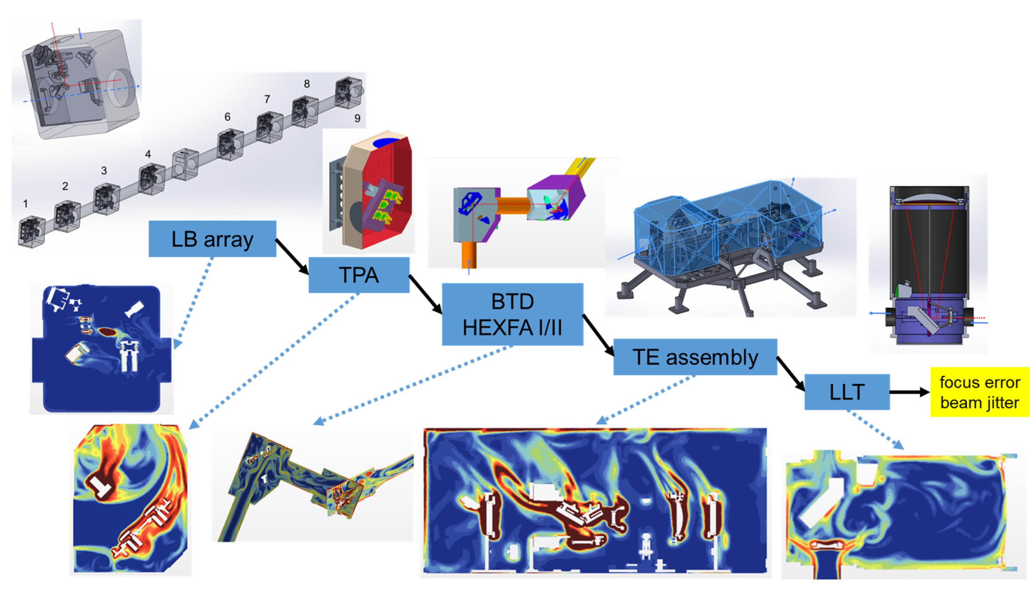
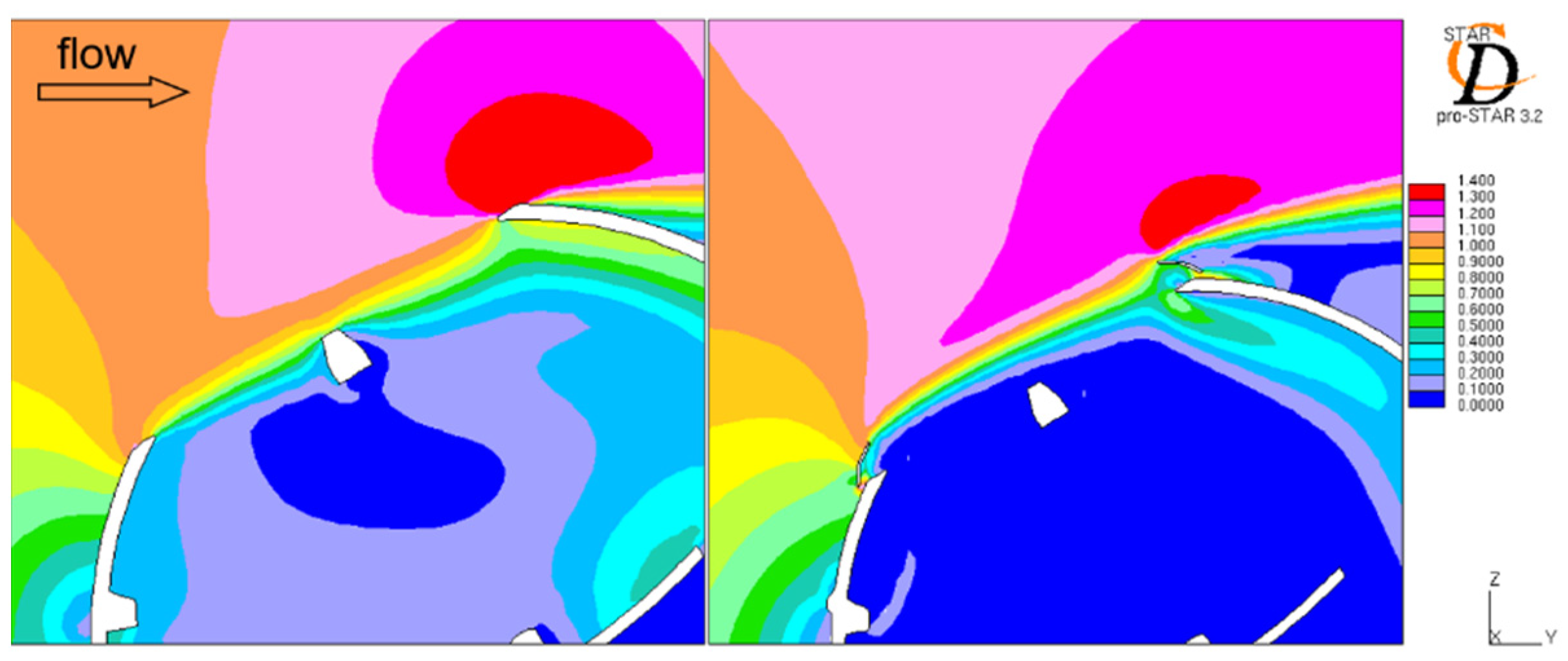
Disclaimer/Publisher’s Note: The statements, opinions and data contained in all publications are solely those of the individual author(s) and contributor(s) and not of MDPI and/or the editor(s). MDPI and/or the editor(s) disclaim responsibility for any injury to people or property resulting from any ideas, methods, instructions or products referred to in the content. |
© 2024 by the authors. Licensee MDPI, Basel, Switzerland. This article is an open access article distributed under the terms and conditions of the Creative Commons Attribution (CC BY) license (https://creativecommons.org/licenses/by/4.0/).