1. Introduction
Although curved beams have been in existence for centuries, minimal guidance has been available on the design of curved steel elements. The fabrication of curved steel beams began in the 19th century when steel members were cast in a curved profile or built up from components into a curved profile. Fabrication advanced, utilising three-roll pressing or induction bending in situations where residual stresses were particularly significant or smaller radii were required [
1]. However, the majority of steel used for construction is formed through the use of roller bending, which is a cold process. When curving open sections using cold processes, the flanges exert a significant force on the web, which could lead to local buckling. Therefore, additional rolls are provided inside the tension flange for sections that are susceptible to local buckling (
Figure 1).
Horizontally curved beams experience significant residual stresses due to the manner in which they are formed. A steel member rolled at room temperature experiences mechanical residual stresses (compressive and tensile) that reduce the ultimate strength of the member by increasing its flexibility, which subsequently causes a decrease in buckling strength [
2]. Tensile residual stresses are particularly detrimental as they are often the cause of fatigue failure and stress corrosion cracking, whereas compressive residual stresses can be somewhat beneficial as they can mitigate the origination and propagation of cracks [
3].
Figure 1.
Additional rolls to prevent web buckling on an I-section [
4].
Figure 1.
Additional rolls to prevent web buckling on an I-section [
4].
The main challenge encountered with horizontally curved beams is that due to the geometry of the beam when normal loads are applied, the beam experiences a complex combination of bending, shear, and torsion simultaneously. Torsional moments can be visualised from the deflected shape as the compression flange tends to deflect laterally away from the centre of curvature [
5]. When bending and torsional moments are applied simultaneously to a beam, the coupling of these forces tends to reduce the carrying capacity of the member. Research has found that the behaviour of horizontally curved beams is dependent on the
R/L ratio, which can also be represented as the span angle. It has been noted that when the span angle is less than 1°, the beam responds similarly to a straight beam and is dominated by flexure (bending). When the span angle is larger than 20°, the beam behaviour of the beam is primarily dominated by torsion. When the span angle is between 1° and 20°, both bending and torsion significantly impact the behaviour of the beam [
6].
In straight I-beams, lateral torsional buckling is easily observable through the lateral displacement and rotation of the member. In curved I-beams, however, this behaviour is always present due to the torsional moments experienced. This behaviour was termed lateral–torsional–vertical behaviour by Lee, et al. [
7]. Therefore, due to initial curvature, similar to initial out-of-straightness in columns, bifurcation-type lateral torsional buckling may not be observed in curved steel I-beams. However, it has been noted that, as seen with straight beams, the flexural strength of curved beams decreases for members that are susceptible to lateral torsional buckling [
6]. The effect of lateral torsional buckling is negligible when the angle between torsional restraints is less than 22.5°. Should this angle be larger than 22.5°, the American Institute of Steel Construction (AISC) recommends that the beam be handled as a straight beam with an adjusted lateral–torsional buckling modification factor that accounts for the curvature.
Over the years, numerous researchers have attempted to provide analytical formulae for horizontally curved members; however, very few have focused on equations regarding deflection and rotation. Wong [
8] modified Castigliano’s second theorem, which was originally developed for straight beams, and made it applicable to horizontally curved beams. Castigliano’s second theorem is a strain energy method that is used to calculate deflection. The equation generated can be seen in Equation (1). C
d can be calculated from
Figure 2. It is important to note here that Equation (1) is limited to beams that are fixed on both sides and a point load is applied at the centre point. Dahlberg [
9] created various equations that can be used for various boundary and load conditions. However, these equations are quite difficult to implement and are therefore rarely used in practice. Furthermore, Dahlberg [
9] did not compare the formula with experimental or finite element results.
Castigliano’s second theorem can also be applied to determine the rotation of curved beams; however, this is often even more tedious than the equations necessary for deflection. However, a simplified equation is provided by AISC (Equation (2)). The symbol h
0 represents the height of the member and Δ
max represents the maximum displacement of the member [
6].
This equation is derived using the M/R method, which is used extensively in the design of horizontally curved beams, where the curved beam is modelled as a straight beam with a length equal to the curved member length. The torsional moment is then accounted for by a separate equation:
Various assumptions have been during the derivation of this formula, including that the thickness of each plate element is small relative to the width, which is, in turn, small relative to the span. The stresses due to warping are assumed to be negligible.
Modelling curved beams in FEM causes further complexities. The majority of commercially available software applications model curved beams as a series of straight beams, which provides sufficient accuracy for most design purposes. If the model experiences significant nonlinear behaviour, a convergence study is required in order to optimise the number of elements required, while the development of torsion further complicates the analysis process. Conventional beam finite elements (FEs) cannot be used to model horizontally curved steel I-beams that experience torsion, due to the existence of warping torsion. Conventional beam FEs account only for St Venant stiffness, which causes numerical error regarding computing the torsional deformation. Current beam FEs that incorporate warping stiffness are available; however, these are rarely incorporated in commercially available software and also tend to be less accurate. Three-dimensional FEs such as shell or solid elements are commonly used by researchers attempting to model the behaviour of curved beams. These elements accurately represent torsional behaviour without the need for numerous torsional constants. Previous researchers found that using solid FEs paired with nonlinear analyses led to accurate estimates of experimental results for both ultimate load and midspan deflection ([
10,
11,
12,
13]).
The combination of bending and shear as well as displacements and twisting rotations causes second-order bending actions in the plane of a curved I-beam. With an increase in load, these interactions grow rapidly and may ultimately cause early nonlinear behaviour and yielding, leading to reductions in the ultimate load-carrying capacity of the beam. This therefore necessitates the usage of nonlinear analyses when analysing horizontally curved beams, as opposed to general static (linear) analysis. Given the complexity of the problem, the use of FEs that are integrated with 3D numerical material models is also recommended, as in this research work.
2. Machine Learning Algorithms
This section briefly presents the various ways machine learning (ML) has been used to develop formulae that allow the design or mechanical investigation of civil engineering structures. ML and artificial intelligence (AI) have been implemented over recent decades in different fields as efficient tools used to predict analysis outputs for engineering problems that are deemed computationally demanding and highly complicated to solve analytically. The use of ML has largely eliminated the need for large numerical analysis, as it contains the ability to provide adequate estimates of the desired outputs. The main issue at hand, however, is that to train an ML algorithm, a large enough dataset is required. Therefore, the primary task of the majority of research work at this stage is the generation of datasets for various reinforced concrete and steel-related problems using either physical or validated numerical experiments. A meta-analysis of various case studies was presented by Markou, et al. [
14]; however, the current paper focused on a single mechanical response problem in an attempt to provide a solution to a problem that has never been solved in the past. It is important to note that all ML algorithms that were used to perform the training, testing, and validation for the needs of this research work can be found on GitHub (
https://github.com/nbakas/nbml/, accessed on 21 June 2023), through downloading nbml freeware. Furthermore, the datasets that were developed for the needs of this research work can be found through the following link (
https://github.com/nbakas/nbml/tree/a0d27c94dd590688815180ebf6428963a24ca245/datasets, accessed on 1 July 2024), whereas the proposed models can be developed directly by the reader.
Various ML algorithms were used in this research, namely linear regression (LR), polynomial regression with hyperparameter tuning (POLYREG-HYT), hyperparameter tuning of extreme gradient boosting (XGBoost-HYT-CV), and parallel deep learning artificial neural networks with hyperparameter tuning (DANN-MPIH-HYT). The LR method was used as a point of comparison for the other ML algorithms (Markou, Bakas, Papadrakakis, and Chatzichristofis [
14]).
POLYREG-HYT is useful for generating relatively accurate closed-form formulae and is applied to develop predictive models in higher-order classes. This relatively simplistic method provides a formula based on the nonlinear combination of all independent variables [
14]. This model is based on the creation of nonlinear terms that are based on the independent variables up to the third degree. The algorithm then selects the nonlinear features that correspond to the minimum error. Originally, this methodology was utilised by Gravett, et al. [
15], who made use of a simplistic approach in determining the number of features to use during training. Thereafter, that algorithm was improved and the use of hyperparameter tuning was introduced, as shown in Markou, Bakas, Papadrakakis, and Chatzichristofis [
14], showcasing the proposed ML algorithm that has been used for the needs of this research work. The improved algorithm is outlined in Algorithm 1.
XGBoost-HYT-CV is a modification to the currently open-source extreme gradient boosting algorithm. The original XGBoost is a gradient-boosting library for ML problems such as classifying and regressing. The algorithm implements the gradient boosting framework, which is designed to be fast and scalable, making it suitable for large datasets [
14]. For improving the current XGBoost algorithm, hyperparameter tuning was used. This tuning was found to exhibit accurate results compared to those of deep learning and require less computing demand [
14]. One benefit of this algorithm is its ability to locate and replace missing values in the training and testing datasets.
| Algorithm 1: Feature selection algorithm for polynomial regression [14] |
![Computation 12 00151 i001]() |
The final algorithm to be engaged was DANN-MPIH-HYT, which has the ability to train on both small and large datasets through the use of parallel processing. The algorithm was programmed to train on both computer processing units (CPUs) and graphics processing units (GPUs) and the use of distributed computations was also provided. This led to faster training and testing times when using the algorithm, as deep learning is known to be particularly slow when dealing with training processes, especially in cases where large datasets are used [
14]. A combination of Horovod with MPI was used to optimise the numerical procedure. The Horovod library was implemented for multi-GPU training. Using Horovod, one is able to take a single GPU training script and run it across numerous GPUs in parallel. Through the use of message-passing interface (MPI) commands, each process is initialised and assigned its MPI rank in a straightforward manner, which is achieved in fewer code changes compared with other approaches. Various experimental algorithms were tested by Markou, Bakas, Papadrakakis and Chatzichristofis [
14] on the Cyclone Supercomputer, utilising PyTorch for computer vision as well as regression tasks, highlighting the efficiency of data parallelism.
ML combined with FEM modelling has been used to create accurate formulae for various engineering applications in recent years. Markou and Bakas [
16] created formulae to determine the shear capacity of concrete slender beams without stirrups. In their research work, a total of 35,849 beams were created and four ML algorithms were used, namely linear regression, polynomial regression, XGBoost, and deep learning neural networks. In that study, it was noted that the XGBoost algorithm was the most accurate, boasting an error of 5.82%. A similar methodology was followed by [
17,
18,
19,
20], where design formulae and predictive models were developed in relation to RC and steel structural problems. In this context, the current research work validates numerical models through the use of results from experiments conducted on curved steel I-beams at the laboratories of the University of Pretoria, and thereafter, the development of a relatively large dataset through nonlinear analyses is described. The next step will involve the development of the proposed predictive models that are validated and presented in the present paper.
3. Experimental Investigation
Experimental studies were performed in order to validate the finite element models that were used to develop the datasets for the needs of this research work. Experiments were also used to determine the appropriate finite element type that would yield the most accurate results regarding the deflection and rotation of the I-beam. The experiments involved the investigation of a horizontally curved steel I-beam (IPE 100) where the two ends were fully fixed and a vertically upward load was applied at the midspan. The results measured were vertical deflection at the midspan, rotation at the midspan and quarter points, and strains at the midspan and the support.
The beam that was analysed was a 3.5 m long IPE100 beam. This beam was selected to minimise the applied forces in order to maintain a safe working environment. A simplified schematic outlining how the beam was supported and loaded can be seen in
Figure 3.
To create a fully fixed support, the cross-section of the IPE 100 beam was welded onto two 12 mm thick plates. These 12 mm thick plates were then welded onto a stiff beam, which was then bolted onto the test floor using M24 Gr8.8 bolts. The entire system was assumed rigid and minimal deflections and rotations were expected at this point. Additional linear variable differential transformers (LVDTs) were placed at the supports. A schematic of the support conditions as well as a photograph can be seen in
Figure 4 and
Figure 5, respectively.
A simple load application mechanism was used, which allowed a quicker and easier test set-up. The beam was loaded with a 40 mm steel bar that had a flat edge. This flat edge was loaded onto the beam using an overhead crane. The load cell then calculated the load experienced by the beam every 100 milliseconds, which was seen to provide sufficient data for analysis purposes. The loading equipment had a capacity of 50 tonnes, which was sufficient for the expected failure load of the beam. The steel bar also allowed the beam to rotate freely at the point of load application, which was required given the large expected rotations of this horizontally curved beam.
LVDTs were used to measure beam deflection only in the vertical direction. Two different LVDT types were used, one with a 250 mm range, which was placed at the supports and the other with a 1000 mm range, which was placed at the midspan. The LVDT at the midspan was placed 160 mm away from the point of load application so measurements could be taken at the same position as the strain gauges. The strain gauges were offset in order to not be influenced by the applied point load. LVDTs were used due to their high accuracy and good long-term stability as opposed to potentiometers, which have lower accuracy and precision but are typically more versatile. A schematic of the placement of LVDTs can be seen in
Figure 6.
Inclinometers were used to measure the rotation along the beam as well as across the beam. Two dual-axis inclinometers were used. The inclinometers used made use of an electrolytic level which was capable of measuring inclination along two axes (pitch and roll). One inclinometer was placed 100 mm from the point of load application but on the opposite half of the beam from where the LVDT and strain gauges were placed, and the other was placed at the quarter point of the same half. A schematic outlining the position of the inclinometers can be seen in
Figure 7.
The majority of the setup of the instrumentation involved accurately placing the strain gauges. Strain gauges are very sensitive. Therefore, the surface where a strain gauge is applied is required to be extremely smooth and free of all impurities prior to the placement of the strain gauge. The placement of these strain gauges was critical so that comparison between the strain gauge and the FE analysis could be as accurate as possible. This was particularly true for the strain gauges placed at 45°, which were required to accurately measure torsional strain within the beam. A total of 16 strain gauges were used to measure the strain at various points on one half of the beam. At the midspan, only longitudinal strain gauges were provided at the top and the bottom flange. These longitudinal flanges were placed at the far edge of the beam to read the maximum longitudinal strain at the midspan. The same setup was followed at the support, which led to another four longitudinally placed strain gauges being placed at this point. Two strain gauges were also placed transversely at the top and bottom flanges to investigate the shear flow in the beam. A further two vertical strain gauges were placed on either side of the web to measure the shear flow of the beam across the web. Four diagonal strain gauges were placed to measure the torsional stresses experienced at these points. A schematic outlining the position of the strain gauges can be seen in
Figure 8.
All instrumentation was connected to an HBX Quantum logger. This logger allowed conversion from voltage to the appropriate units for the various instrumentation after calibration (e.g., millimetres for the LVDT, kilonewtons for the load cell, and micrometres/metres for the strain gauges). During the experiment, the load was applied to the beam in increments up to the final failure load past the point of yielding. During loading, a video was taken to record the experiment, which was used for verification when analysing the results. Photos were then also taken after the final load was applied and yielding had been experienced for further analysis (
Figure 9).
4. Analysis of Experimental Results
During testing, a total of five variables were measured. These variables were the load applied at the midspan, the displacement, the tilt/rotation, and the strain. The initial readings prior to the load application were taken as a reference point for all future readings. As previously mentioned, the load was applied incrementally in steps of 3 kN. This was carried out so it could be accurately determined at what load yielding occurred (through measuring permanent deformation). It was noted that after the 12 kN load was removed, permanent deformation occurred at the midpoint of the beam. The deflection for this load was approximately 55 mm.
The deflection measured at the supports was negligible, reaching up to 0.07 mm (upwards). This was seen as negligible and therefore was not factored into the calculations of the midspan deflection.
Figure 10 shows the load–deflection curve of the beam. Results showed that the beam deflected linearly up to 55.05 mm at a load of 12.42 kN. The experiment was stopped right at the point of yielding; therefore, a plateau is not indicated in this graph, which would be a further indication that yielding had occurred.
When investigating the tilt results, errors were noted. The results showed that tilt did not consistently increase as load increased. At some points, a decrease in tilt was measured with an increase in load. This can be seen in
Figure 11, where it can be seen that as the load increased from 2 kN to 4 kN, the tilt was measured to have decreased slightly. Practically, this is not possible. It is believed that this error was due to incorrect use of the measuring apparatus. The apparatus used to measure tilt made use of an electrolytic level. Electrolytic levels are typically poor when it comes to dynamic/cyclical loading, due to the conductive fluid found within the sealed glass. These results can therefore be used to obtain a rough estimate of how tilt increases as the load increases; however, these results cannot be used to determine the accuracy of FE models or analytical formulae. A line of best fit has been included in
Figure 11 for further interpretation, which shows that tilt increased as load increased.
The strain results were quite interesting and showed the implication of the support conditions utilised. The support was intended to be fully fixed; however, practically, the support behaved in a way between that of a fully fixed connection and a torsionally pinned connection, as was seen with the strain gauge results. The strain gauge pattern was symmetrical with the cross section (both vertically and horizontally); however, the results were not seen to be perfectly symmetrical. The major reason for the discrepancies was most likely to have been due to inaccuracies during the setting out of the strain gauges. Material and geometric imperfections also played a role. The strain gauge results can be seen from
Figure 12,
Figure 13 and
Figure 14.
5. Comparison of Experimental Data with Finite Element Analysis Results
Various FE models were used and compared to determine which model most accurately represented the behaviour of the experimental beam. The focus was to determine the optimum FE model to be used for the development of the datasets. The datasets were used to train various ML algorithms for the development of the proposed predictive models related to the calculation of the ultimate strength of curved steel I-beams that are fixed at their ends and the respective deflection.
CivilFEM 2021 was used to develop the numerous FE meshes that were used to construct the dataset. This software was selected due to its interface, which allowed the creation of curved steel I-beam meshes in an automated manner. Solid and shell FEs were considered in this research work, where the mesh size was determined based on a previous research study where a mesh sensitivity analysis was conducted by the authors [
21]. Linear and quadratic elements were also considered for each of the FEs used to reproduce the experimental results. It is important to note at this stage that [
21] used experimental results found in the literature to calibrate their model that involved steel I-beams with a different support system compared with the fixed-end beams that are investigated herein. That pilot project showed that hexahedral isoparametric FEs were able to accurately reproduce experimental results [
21].
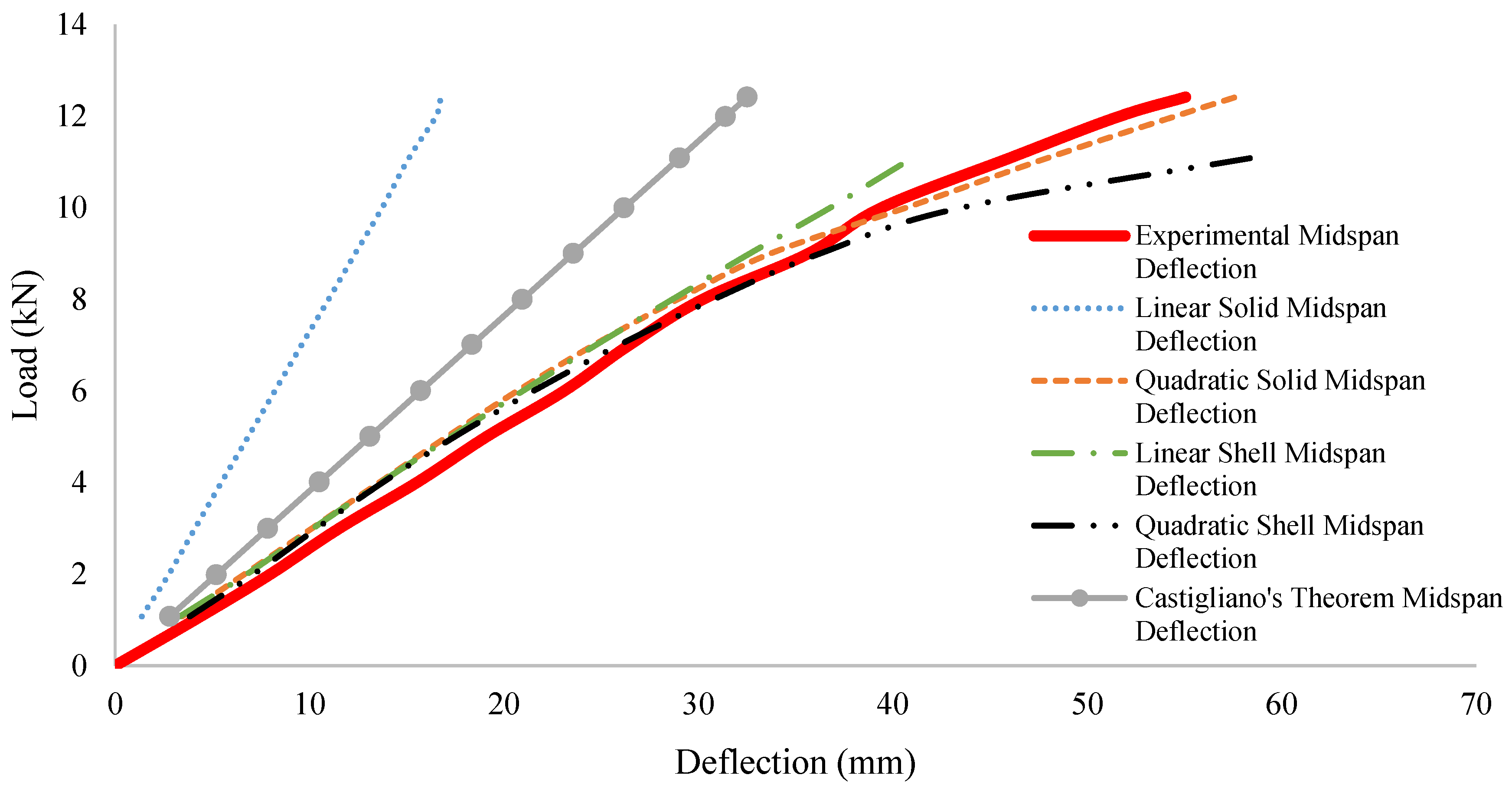
Therefore, a total of four models were created for the needs of this research work, namely, a linear solid element, a quadratic solid element, a linear shell element, and a quadratic shell element. All material-related parameters were kept constant between the four models to maintain consistency. A typical nonlinear material model with anticipated bilinear behaviour was assumed. The hardening type selected was isotropic, indicating that yielding occurred when the effective or equivalent stress was equal to the specified yield stress. This selected yielding criterion was set to be that of von Mises. Furthermore, the material properties were assumed to be that of an S355 steel material (355 MPa yield stress, 210 GPa elastic modulus, a Poisson ratio of 0.3, and a density of 7850 kg/m3). The experimental deflection and rotation at the midspan were then compared with the midspan deflection and rotation calculated using the various FE models. Analytical formulae were also included for comparative purposes.
Figure 15 shows that the linear solid FE derived the worst prediction when estimating midspan deflection. The analytical method, Castigliano’s second theorem, was also unable to accurately represent the behaviour of the beam and performed quite poorly compared with the more advanced FE models. The quadratic solid model most accurately calculated the midspan deflection, with an average error of only 1.83 mm. A summary of the computed mean absolute error (MAE) can be seen in
Table 1.
Furthermore, the resulting section rotations can be seen in
Figure 16. Similar to the deflection results, experimental data and the results derived from FE analyses were compared with those of a commonly used analytical method, as discussed previously (Equation (2)). The experimental deflection was used as an input to achieve the highest accuracy possible when implementing the analytical method. Due to the fact that solid FEs do not contain rotational degrees of freedom, the rotation was calculated from first principles through making use of the vertical deflection at opposite ends of the bottom flange and using trigonometry to calculate the rotation. This method only holds given that the cross-section does not warp significantly. From the graphic, it was noted that the linear solid FEs provided the least accuracy, underestimating the midspan tilt quite significantly.
The M/R performed slightly better compared with the linear solid Fes; however, these results were still exceedingly conservative compared with the more advanced FE models. The more advanced FE models correlated well with the line of best fit of the experimental data. However, it seems the quadratic shell model was more accurate up until approximately 10 kN. From 10 kN to failure, the linear shell and the quadratic solid models both displayed lower errors compared with the experimental data. A summary of error metrics (MAE) can be seen in
Table 2.
It is therefore concluded that FE models with the numerical modelling technique as outlined in this section are capable of accurately representing the behaviour of horizontally curved steel I-beams. These models have also been shown to outperform quite significantly the existing analytical formulae for estimating both deflection and rotation. It was noted that of all the FE models, the quadratic solid FE performed best in both estimating deflection and rotation. Therefore, the numerical modelling technique outlined in this section was utilised in developing a large dataset as described in the subsequent sections.
6. Numerical Campaign
A relatively large dataset consisting of 864 models was created through the use of CivilFEM. A total of six sections were considered, namely, IPE100, IPE200, IPE300, IPE400, IPE500, and IPE600. This was done to encompass the entire IPE section list according to European standards. The variables considered were the moment of inertia around the x axis (Ixx), the moment of inertia around the y axis (Iyy), polar moment of inertia (J), section height (h), section width (b), section area (A), beam curved length (L), beam radius of curvature (R), material yield strength (fy), material Young’s modulus (E), material Poisson ratio (v), and material shear modulus (G). For each section considered, three yield strengths were assumed (235 MPa, 275 MPa, and 355 MPa), to account for the various structural steel strengths commercially available in South Africa. Three Young’s moduli were considered, namely, 190 GPa, 200 GPa, and 210 GPa, to account for variances in material stiffness. The Poisson ratio was fixed at 0.28 and the equation of G was calculated based on E and v. Four lengths and four radii were considered per section in order to cover the broad range of geometries that the proposed predictive models will be applicable for. Given that R/L ratios have been found to control the behaviour of curved beams, four specific R/L ratios were considered on all beams, namely, R/L = 1, 2, 4, and 8. All the beams were fully fixed on both ends and a load was applied normally downwards at the midspan.
To maintain consistency, the models were automatically generated using a Python script within CivilFEM. This ensured all material and geometrical properties were maintained and only a single variable was modified, allowing automatic mesh generation. A Python script was developed and optimised to ensure consistency and minimise running time through decreasing the number of variables and the overall performance of the code. The models all made use of quadratic solid elements with a mesh size of up to 50 mm. A typical nonlinear material model with predicted bilinear behaviour was assumed. The hardening type selected was isotropic, which indicates that yielding occurred when the effective or equivalent stress was equal to the specified yield stress. This selected yielding criterion was set to be that of von Mises.
Table 3 indicates different statistical parameters, including skewness. A value of 0 indicates that the dataset contained no skewness and had a perfectly normal distribution. According to Aminu and Shariff [
22], a range from −3 to 3 can be considered as a cutoff, and based on this, the results show that the data were not significantly skewed. Kurtosis is another parameter that assists further in determining whether a dataset is normally distributed or not. This is performed by determining whether a dataset is “heavy-tailed” or “light-tailed”. “Heavy-tailed” implies that a dataset contains numerous data points in outlier positions, whereas a “light-tailed” dataset contains minimal to no outliers. Once again, there is no accepted convention on what is deemed “heavy-tailed”; however, Aminu and Shariff [
22] state that a range from +10 to −10 is deemed light-tailed and contains minimal outliers. In this context, it was observed that the dataset created for the needs of this research work contained minimal outliers with a good distribution.
The correlation matrix for the displacement dataset can be found in
Figure 17a and for the failure load dataset in
Figure 17b. It was clear from the correlation matrix results that all cross-sectional properties had a strong positive correlation with the midspan deflection and the failure load. It was also clear that, of all the properties, the curved length had the largest correlation with the midspan vertical deflection. This implies the potential to translate to positive results in the sensitivity analysis; this is discussed in
Section 7.
7. Machine Learning Training and Testing
This section outlines how numerous ML algorithms were applied in order to create formulae that can outperform current analytical methods used to estimate the deflection of horizontally curved steel I-beams. The ML algorithms considered were linear regression (LR), polynomial regression with hyperparameter tuning (POLYREG-HYT), deep artificial neural networks with MPI, Horovod, and hyperparameter tuning (DANN-MPIH-HYT), and extreme gradient boosting with hyperparameter tuning and cross-validation (XGBoost-HYT-CV) [
14]. It must be noted here that for the ML analyses performed, 85% of the dataset was used to train the ML algorithm and 15% was used for testing. The performance of ML algorithms varies; therefore, to quantify accuracy, numerous error metrics were considered. The error metrics considered in this research work were the mean absolute percentage error (MAPE), the mean absolute mean percentage error (MAMPE), the mean absolute error (MAE), and the root-mean-square error (RMSE). The Pearson correlation coefficient was also considered (R) for determining the similarity between the PV (predicted value) and the DV (dependent variable). An in-depth discussion of the error metrics can be found in [
23].
7.1. Proposed Predictive Models for the Case of Deflection
This section outlines the midspan deflection predictions provided by the various ML algorithms. The numerically obtained error metrics were analysed to determine the performance of the various proposed predictive models. The correlation for the train and test datasets can be seen in
Figure 18,
Figure 19,
Figure 20 and
Figure 21.
LR and POLYREG-HYT are the only ML algorithms considered in this study that are capable of providing closed-form formulae. Equation (3) shows the formula generated with the LR algorithm, which can be used to estimate the vertical midspan deflection, whereas Equation (4) provides the proposed predictive model derived using POLYREG-HYT. When implementing the formulae, all cross-sectional properties are in mm/mm
2/mm
3/mm
4, and the span is given in m. The yield strength is provided in MPa and the Young’s modulus in GPa.
Visually, it was difficult to discern which ML algorithm performed the best. Therefore, as previously mentioned, numerous error metrics were used to measure the performance of the various algorithms.
Table 4 summarises the results. As can be seen, XGBoost-HYT-CV was the most accurate proposed model when looking at the training dataset, whereas when comparing the error metrics obtained from the testing dataset, that was not the case. The DANN-MPIH-HYT proposed predictive model was found to be slightly more accurate. It should also be noted that, even though DANN-MPIH-HYT was the most accurate in the testing phase, this algorithm did require the longest computation time (27 times slower).
Ultimately, it was apparent that accurate formulae can be created using ML algorithms. A later section of this paper compares these results with out-of-sample data, further validating the proposed predictive models’ ability to capture unknown results.
Sensitivity analyses were conducted on each of the independent variables to determine which variable affected the dependent variable the most. This will assist future studies in determining which variables to exclude in order to increase efficiency in the proposed predictive models. This analysis also provides engineers with a deeper understanding of the behaviour of horizontally curved steel I-beams.
Figure 22 summarises the findings of the sensitivity analysis. As can be seen, the three most influential variables on midspan vertical deflection were the curved length (
L), the moment of inertia around the minor axis (
Iyy), and the radius of curvature (
R).
L was by far the most influential variable, according to the obtained results. The cross-section area, cross-section width, and cross-section height had practically no impact on the midspan deflection, according to the sensitivity analysis performed for the needs of this research work related to the beam deflection.
It is important to show here that the predictive models did not overfit and that the solution obtained through the ML analysis led to an objective predictive model that did not overfit. In addition to the validation presented in
Section 8,
Figure 23 shows the tuned cross-validation histories for the DANN-MPIH-HYT and the XGBoost-HYT-CV ML algorithms. It was evident that the algorithms were able to derive models that were optimised through the training and testing procedure.
7.2. Proposed Predictive Models for the Case of Failure Load
This section outlines the failure load predictions provided by the various ML algorithms. An analysis was conducted to determine the performance of the various proposed predictive models. The correlation for the train and test datasets can be seen in
Figure 24,
Figure 25,
Figure 26 and
Figure 27.
As stated previously, it was necessary to use error metrics to determine which ML algorithm performed the best. Therefore, a summary of error metrics can be seen in
Table 5. As can be seen, the proposed XGBoost-HYT-CV model was the most accurate when looking at the training and testing datasets. This indicates the fact that no ML algorithm was capable of providing accurate results for all datasets, and different algorithms were used in allocating the best fit to a specific dataset.
For the cases of the closed-form solutions, Equation (5) shows the formula generated with LR, and Equation (6) provides the proposed predictive formula generated through the POLYREG-HYT ML algorithm:
Sensitivity analyses were also conducted on the failure load dataset. A graphical summary of the findings can be seen in
Figure 28. As can be seen, the three most influential variables on the midspan failure load were the moment of inertia around the major axis (
Ixx), the curved length (
L), and the radius of curvature (
R).
Ixx was by far the most influential variable, due to the fact that as the stiffness of the beam in bending increased, a larger load was required to reach failure. The cross-sectional area (
A), flange width (
b), cross-sectional height (
h), polar moment of inertia (
J), and moment of inertia around the minor axis (
Iyy) had practically no impact on the failure load according to the XGBoost-HYT-CV ML algorithm. These findings can be used to create an improved, simpler dataset in the future.
Before moving to the validation section presented next,
Figure 29 shows the tuned cross-validation history for the case of the DANN-MPIH-HYT and XGBoost-HYT-CV algorithms resulting from the analysis. Once more, it is easy to observe the numerical response of the two histories that converge to R
2 = 1.0, which represents maximum data correlation.
8. Validation
This section outlines the process of validation that was performed through the use of out-of-sample FE models. The validation aimed to evaluate the proposed predictive models’ abilities to capture data that were not used during training or testing. It must be noted here that the ML algorithms were trained on IPE sections (IPE 100, IPE 200, IPE 300, IPE 400, IPE 500, and IPE 600) of various geometries. For validation purposes, it was decided to use sections as per the
South African Steel Construction Handbook (SASCH). The sections considered were 203 × 133 × 25, 305 × 165 × 40, and 457 × 191 × 67. Therefore, the proposed predictive models had never been exposed to this type of sectional geometry. Additionally, out-of-sample R/L ratios of 2.5 and 5 were considered and the overall span of the section varied depending on the section depth. Out-of-sample yield strengths of 285 MPa and 325 MPa were considered and the Young’s modulus values considered were 195 GPa and 205 GPa. This led to a total of 48 out-of-sample beams being created for validation purposes. The descriptive statistics relating to the new validation dataset can be seen in
Table 6.
8.1. Validation of Deflection ML Results
The proposed predictive models that were developed to estimate the deflection of the beams were used to predict the deflections of the out-of-sample data. This section focuses only on the two algorithms, namely, DANN-MPIH-HYT and XGBoost-HYT-CV, that were found to outperform the rest of the ML-generated predictive models. Correlation plots of the two ML models can be seen in
Figure 30 and
Figure 31. These results were compared with the current analytical method, Castigliano’s second theorem. The graph showcasing the correlation of Castigliano’s second theorem can be seen in
Figure 32.
A summary of the error metrics of all ML algorithms can be seen in
Table 7. As can be seen, the DANN-MPIH-HYT algorithm outperformed all ML algorithms and the currently used analytical formula. The POLYREG-HYT formula performed the worst. This poor performance was attributed to over-fitting, as the LR formula was quite accurate. It should be noted that even though these results were verified using FEM models, the FE modelling technique used was experimentally verified using an experimental beam where the error experienced was negligible.
8.2. Validation of Failure Load ML Results
The proposed predictive models previously discussed were used to predict the failure load of the out-of-sample data. This section outlines the findings. No analytical formulae are discussed in this section, as the focus of this article is more on deflection estimation and not failure mode investigation. Due to the complexities associated with the failure modes of horizontally curved beams, numerous equations were consulted, and their inclusion would overwhelm the article. The focus herein is on DANN-MPIH-HYT and XGBoost-HYT-CV since they were found to outperform the other predictive models. Correlation plots can be seen in
Figure 33 and
Figure 34.
The results paint a different picture from what was seen during training and testing. The XGBoost-HYT-CV did not seem to achieve better results than those generated with the DANN-MPIH-HYT algorithm; however, a closer look at the error metrics was required. A summary of the error metrics can be seen in
Table 8.
As can be seen, the correlation was significantly worse and all the error metrics showed that the predictions provided through the XGBoost-HYT-CV were less accurate than the predictions provided through the DANN-MPIH-HYT algorithm. This is the same phenomenon as was experienced in the deflection dataset where the DANN-MPIH-HYT algorithm performed better with the out-of-sample data compared with all the other ML algorithms. Therefore, the extended duration required to train the DANN-MPIH-HYT algorithm can be said to translate to improved accuracy during validation.
9. Conclusions and Recommendations
This study showed that FE modelling was able to replicate the experimental results acquired with horizontally curved steel I-beams. For the needs of this research work, an experiment was performed that involved the loading of an IPE100 curved steel I-beam under a vertical load. The experimental data obtained were then used to validate numerical models through the use of CivilFEM software. The usage of quadratic solid FEs with a hexahedral mesh size of 50 mm as well as appropriate material constitutive models paired with nonlinear analyses led to the most accurate results when compared with the experimental data.
A parametric investigation was conducted in which it was noted that the FE modelling technique outlined in this research work was capable of accurately estimating the midspan deflection and rotation of horizontally curved steel I-beams. The MAE was noted to be 3.32% when estimating deflection and 9.17% when estimating rotation, which far outperformed analytical methods, which had an error of 19.80% when estimating deflection and 16.07% when estimating rotation.
The experimentally validated model was then used to develop numerous FE meshes that were analysed under ultimate limit state loading conditions. The numerically obtained results were used to develop a large dataset. A total of 864 models were created that encompassed the entire IPE cross-section list (IPE100 to IPE600). A total of 10 independent variables were considered in this study.
Numerous ML algorithms were used, namely, LR, POLYREG-HYT, DANN-MPIH-HYT, and XGBoost-HYT-CV, for developing the proposed predictive models. During the validation phase, experimentally validated FE models that were outside the training dataset were created to validate the various proposed predictive models proposed in this research work. To further evaluate the accuracy of the available analytical methods for computing the deflection and ultimate load of curved steel I-beams, the validation data were used to assess Castilgiano’s analytical formulae as well. According to the numerical findings, the DANN-MPIH-HYT algorithm was the most accurate in estimating both deflection and failure load. When estimating deflection, the DANN-MPIH-HYT proposed predictive model had a MAMPE of 16.19%. This was found to be a significant improvement compared with the analytical method, Castigliano’s second theorem, which derived an extremely large MAMPE of 126.23%, highlighting the need for more accurate and objective predictive models. It is also safe to conclude that based on the findings of this dissertation, the proposed ML-generated predictive models are far more accurate than the current analytical methods for estimating the deflection of curved steel I-beams.
In addition to the above, when estimating the failure load of curved steel I-beams, the DANN-MPIH-HYT generated model was found to be significantly more accurate than the other proposed models. This is most likely to be due to the complexities associated with horizontally curved steel I-beams and the nature of the datasets. Horizontally curved steel I-beams have various failure modes, given that they can fail due to flexure, torsion, shear, or a combination of these. The beams may also fail due to lateral torsional buckling. Therefore, a larger dataset is required for the ML algorithms to derive the patterns that are connected to the failure modes of the beams. At this stage, the international literature includes numerous equations for each of the failure modes. Therefore, there is no individual formula to compare the estimates with. It is believed that the DANN-MPIH-HYT algorithm, which resulted in a MAMPE of 22.42%, can be further improved in the future by either increasing the dataset or providing different formulae for the different failure modes, as is currently the case in all design codes.
Finally, this research study is able to propose, for the first time in the international literature, accurate and objective predictive models that outperform any known formula used to compute the deflection of curved steel I-beams and their ultimate capacity. The largest datasets currently available in the international literature were also developed for the training and testing of the proposed predictive models. This pilot project paves the way for the development of future design formulae that can be more accurately applied to a larger range of beams for different boundary conditions.
This research was limited to evaluating the feasibility of using FE models to estimate the midspan deflection and failure load of horizontally curved steel I-beams with a single point load at midspan and fully fixed at both ends. The development of the datasets foresaw the use of minimum and maximum geometrical features. Therefore, the proposed predictive models should not be used for beams with dimensions that are larger or smaller than the respective maximum and minimum geometrical values of the beams found in the datasets developed herein. Furthermore, recommendations for future work should include the following:
Perform more experiments on curved steel I-beams to further validate the proposed predictive models;
Consider various boundary conditions, such as torsionally pinned beams, and determine the influence this has on deflection, failure load, rotation, and stress distribution. In theory, this should not significantly impact the failure load. However, this is expected to have a drastic impact on the stress distribution and rotation of the section;
Consider various loading conditions, such as uniformly distributed loads;
Consider the impact residual stresses have on stress distribution and investigate whether this has an impact on deflection and failure loads. Residual stresses are far greater in horizontally curved steel I-beams compared with straight beams, due to the initial cold-forming process. Therefore, residual stresses vary depending on the R/L ratio at hand. Currently, there is no formula available in the international literature that allows accounting for how the residual stresses vary throughout the length of the beam and within the cross-section. Therefore, a detailed investigation is required.
Develop an accurate formula to determine the midspan rotation of horizontally curved steel I-beams using a relevant dataset.


