A Novel Mixed Finite/Infinite Dimensional Port–Hamiltonian Model of a Mechanical Ventilator

Abstract

Mechanical ventilation is a life-saving treatment for critically ill patients who are struggling to breathe independently due to injury or disease. Globally, per year, there has always been a large number of individuals who have required mechanical ventilation. The COVID-19 pandemic brought to light the significance of mechanical ventilation, which played a significant role in sustaining COVID-19-infected critically ill patients who could not breathe on their own. The pandemic drew the attention of the world to the shortage of ventilators globally. Some of the challenges to providing an adequate number of ventilators include: increased demand for ventilators, supply chain disruptions, manufacturing constraints, distribution inequalities, financial constraints, maintenance and logistics difficulties, training and expertise shortages, and the lack of design and development of affordable mechanical ventilators that satisfy the stipulated requirements. This research work presents the formulation of a detailed Port–Hamiltonian model of a mechanical ventilator integrated with the human respiratory system. The interconnection and coupling conditions for the various subsystems within the mechanical ventilator and the coupling between the mechanical ventilator and the human respiratory system are also presented. Structure-preserving discretization is provided alongside numerical simulations and results. The obtained results are found to be comparable to results presented in the literature. Future work will include the design of suitable controllers for the system.

1. Introduction

The World Health Organization (WHO) has “access to oxygen” on its model list as one of the essentials required by an individual, especially when they are in a critical condition health-wise and are unable to breathe on their own. Oxygen is the only listed medicine that does not have a substitute. Access to oxygen even after the worldwide pandemic is still a major dilemma in middle- and low-income countries [1]. A mechanical ventilator is a medical device that is employed to assist patients in cases where their respiratory system is not functioning well and, thus, the patient has challenges with breathing or has shortness of breath. A mechanical ventilator can also be used in cases where a patient has been sedated and is undergoing surgery.

The basic operation of a mechanical ventilator is to control a high-pressure region during the inspiration stage. In the inspiration stage, the mechanical ventilator is paused. During expiration, air flows out due to the lung’s natural recoil, which creates higher pressure in the alveoli. Due to the high demand for mechanical ventilators both in the past and at present, it is imperative that efficient and affordable mechanical ventilators be researched, modelled, designed and implemented. To ensure that robust mechanical ventilators are designed, it is important to formulate new models that can be used in the research and testing stages of mechanical ventilators.

1.1. Mathematical Models of the Respiratory System

Sound mathematical formulations of the underlying physics of the respiratory system are very important for understanding the anatomy and physiology of the organs. Classical modelling methodologies that employ a physiological or clinical perspective have been previously used mainly for data-fitting for single-compartment model parameters: for example, [2]. Human lungs are usually mathematically viewed to be made up of intricate branching networks of compliant tubes spanning a broad range of scales and flow regimes. The flow may be a highly pulsatile flow or an almost laminar diffusion-dominated process. Flow enters a sponge-like microstructure of lung tissue from the terminal branches of the airway. The lung tissue material’s behaviour is very nonlinear, and for efficient gaseous exchange, the topology is optimized with small embedded blood vessels. Current research developments in the mechanical and mathematical modelling of the lungs have mainly focused on studying isolated effects that are difficult to understand and assess in vivo. These studies seek to advance medical imaging and functional diagnostics and assist with patient-specific treatment planning and optimization. Bates [3] used a system identification approach to provide a mathematical description of lung mechanics, with evolving intricacies in the mathematical formulations. This ranged from single linear compartments to generalized multi-compartmental models. Maury [4] further developed the concept proposed by Bates [3] and described the lung as a resistive tree. Various levels of description have been proposed, including lumped models with a small number of parameters described by ordinary differential equations (ODEs) up to infinite-dimensional models based on partial differential equations (PDEs). Resistive networks and how they can be used to investigate the dependence of the lung’s resistance on geometrical characteristics have also been presented. Analyses of the various models from a theoretical perspective have been provided. The approximate solution techniques that have been provided have shown good correlation with experimental measurements. Other researchers that have proposed similar works are Burrowes et al. [5], Tawhai et al. [6], and Berger et al. [7]. Research has also been conducted by Roth et al. [8] using Navier–Stokes equations for fluid flow from a very mathematical perspective. This research work also provides comprehensive and computationally fully resolved fluid representations of human respiratory models or parts thereof. Solutions of the three-dimensional Navier–Stokes equations on rigid geometries have also been formulated. Information from medical imaging alongside the fluid domain have been used to formulate real fluid–structure interaction effects [8]. As an approach for replicating real fluid–structure effects, techniques have been developed and published that demonstrate this concept in the fluid domain by the application of data from medical imaging information. To quantify particle deposition or drug delivery in the lower and upper airways and for investigation of patterns in the lungs such as jets or vortices, a fully resolved fluid model may be used. Such models are very complex, and in most cases, only parts of the human respiratory system are investigated, thus eliminating the important impact of the entire organ. A holistic human respiratory system model requires a consistent, physiologically realistic representation of the respiratory mechanics in addition to the purely mechanical or structural aspects because the basic physics of respiratory mechanics are governed by the interaction of the fluid with the anatomy. The normal functioning of the lung is possible due to the deformation of the associated muscles, airway tree and lung tissue. Indeed, tissue properties have an influence on airflow and the processes that occur during air transportation: for instance, during gaseous exchange or aerosol transportation.

1.2. Related Works

Tran et al. [9] conducted research work with the main goal of designing, controlling, modelling, and simulating a mechanical ventilator that is lightweight, portable, and suitable for use at home. Tran et al. [9] modelled a mechanical ventilator as a voltage source. El-Hadj et al. [10] applied the fluid–structure interaction (FSI) to couple the computational fluid dynamics used for fluid flow with finite element analysis for the solid domain. This facilitated the investigation of fluid behaviour, structural behaviour, and interactions. Two designs were proposed for the mechanical ventilator. The first design was reported to be uncontrollable, and the second design considers computational fluid dynamics (CDF) with a moving boundary applied to a piston-cylinder-based ventilator. Tharton et al. [11] designed and developed a ventilator prototype to be used by professionals in medical emergencies and in any other context where the regular ventilator is not available. A mechanical ventilator was modelled using a crank rocker mechanism in order to meet specific requirements for mechanical ventilator design. Pivk et al. [12] developed an empirical model for a low-cost mechanical ventilator by observing the response of each of the ventilator subsystems. The current progress made globally in the development of affordable and effective designs is important. However, research in mechanical ventilator development lacks model development. The Port–Hamiltonian approach applied in this research work acts as a modelling template for future energy-based mechanical ventilator modelling and design. Lagrangian modelling and Kane’s approach do not emphasize energy routing in the system through a Dirac structure. Kane’s method is also limited with regard to modelling of the fluid interaction of the mechanical ventilator–human respiratory system. It is important to develop designs that rest on a solid understanding of a significant aspect of the design. Naggar [13] developed a piecewise model of a mechanical ventilator that describes the artificial behaviour of a mechanical ventilator. A pressure-controlled ventilator was created and simulated. The mechanical ventilator was modelled using a periodic function with inequalities to control the beginning of the inspiration and expiration periods. Shi et al. [14] developed a mathematical model of volume-controlled mechanical ventilation. The model is viewed as a pneumatic system wherein the ventilator is regarded as an air compressor. The exhalation valve is considered a throttle. The compressor and the container represent the ventilator. Naggar et al. [15] proposed an integrated mathematical model of the mechanical ventilator and the lung. Linear quadratic and exponential equations were used to model the system. The integrated model was used to simulate volume-controlled artificial ventilation. Giri et al. [16] proposed a simplified design of a mechanical ventilator to reduce cost and automate the mechanical ventilation process. The proposed design was simulated on the MATLAB platform. Hannon et al. [17] reviewed the progress in mathematical modelling and simulation of human anatomy, physiology, and pathophysiology using computers in the context of mechanical ventilation. This study emphasized the clinical applications of computer simulations in various disease states. The research work further discussed the present constraints and the possibility of in silico modelling. There are currently no existing Port–Hamiltonian models of mechanical ventilators.

1.3. Applications of Integrated Mechanical Ventilator–Human Lung System Models

Integrated mechanical ventilator–human lung system models can be used to simulate the behaviour of the respiratory system and to study the effects of mechanical ventilation on lung function. These models have several applications in research, education, and clinical practice. Overall, integrated mechanical ventilator–human lung system models provide a valuable tool for understanding the behaviour of the respiratory system under mechanical ventilation and for developing improved strategies for the diagnosis and treatment of respiratory disorders. The subsections to follow provide examples of applications of integrated models of the mechanical ventilator–respiratory system. In Mehedi et al. [18], the respiratory system was modelled as a combination of the blower-hose patient system with nonlinear lung compliance. There are currently very few studies that have conducted simulations during expiration since the availability of storage for the inhaled volume is required during expiration.

1.4. Motivation of the Port–Hamiltonian Approach

Both the mechanical ventilator and the human respiratory system are multi-physical in nature (they contain components from various domains in physics). As such, a more apt approach to understand the manner in which these systems work, the coupling between them, etc., and, furthermore, to improve the efficiency of mechanical ventilation, is to make use of models that better represent these systems. Thus, a more representative modelling approach would be to account for the multi-physical nature of these systems [19,20]. The Port–Hamiltonian approach for modelling integrated systems has several benefits, including [19,20]:

• The Port–Hamiltonian approach is modular and is based on the topology of the mechanical ventilator and the human respiratory system. Thus, various types of mechanical ventilators and human respiratory systems with different structure/topologies can be simulated/tested numerically under various operating conditions to analyse performance, etc. [19,20].
• The modular nature of the Port–Hamiltonian method, together with its basis in graph theory, means that one can proceed to develop software to automate the modelling of various types of mechanical ventilator/human respiratory system topologies [19,20].
• Properties such as the passivity of the integrated mechanical ventilator–human respiratory system can be shown and studied [19,20].

Currently, there are no energy-based models of MV–patient systems that can be used in systems that have dissipation of energy from the ports. Complex dynamical systems can be modelled and controlled in the Port–Hamiltonian framework because the framework provides a powerful tool for the analysis, modelling and control of such systems. The key attributes of the Port–Hamiltonian (pH) framework are: Firstly, it is established on the multi-domain bond-graph modelling method, which connects various physical elements via ports. The interconnection in the Port–Hamiltonian method is such that there is power conservation. Secondly, there is significance assigned to the energy variables as well as the total energy stored, which is also known as the Hamiltonian and is the foundation for multi-physics system modelling. The Port–Hamiltonian approach provides the basis for understanding energy transfer in the various physical domains that govern the respiratory system. Sampled data can be obtained when the Port–Hamiltonian structure is exploited and preserved in discretization. This research work applies the Port–Hamiltonian system approach to model the MV–human respiratory system. The resulting model explicitly shows the energy storage, energy dissipation and the interconnection underlying the system. The obtained Port–Hamiltonian model has numerous applications: for instance, it may be applied in the design of various medical devices and for respiratory disease diagnostics.

The main contribution in this research work is the development of an integrated Port–Hamiltonian model representation of a mechanical ventilator–human respiratory system. The model consists of electromechanical and electromagnetic components modelled in a finite-dimensional representation and interconnected with fluid components in an infinite-dimensional representation. As a result, this Port–Hamiltonian model is of a mixed finite/infinite dimensional nature. The remainder of this paper is structured as follows: The materials and methods are outlined in Section 2, Section 3 and Section 4 present the detailed Port–Hamiltonian model of a mechanical ventilator and the solenoid valve subsystem. Section 5 and Section 6 give the model network topology and model interconnection with coupling conditions. Section 7 and Section 8 show the structure-preserving discretization, results and discussion. Finally, the conclusion and recommendations are presented in Section 9.

2. Materials and Method

This section presents the mathematical preliminaries of the Port–Hamiltonian approach that are followed in later sections. These definitions are standard definitions from the literature and are mostly derived from the following references: [21,22,23].

Definition 1.

(Dirac structure):

A Dirac structure (DS) is a pair of elements, $f\in {\mathbb{R}}^n$ and $e\in {\mathbb{R}}^n$, that satisfies the set:

$$\begin{array}{c}\hfill \mathcal{D} :=\left\{(f,e)\in \mathcal{D},(\widehat{f},\widehat{e})\in \mathcal{D}\left|e^{\mathsf{T}}\widehat{f}=-{\widehat{e}}^{\mathsf{T}}f\right.\right\}.\end{array}$$

The DS is a subset $\mathcal{D}\subset \mathcal{F}\times \mathcal{E}$, where $\mathcal{F}$ and $\mathcal{E}$ represent the flows and efforts, respectively.

The DS in electric circuits can be represented as:

Proposition 1.

The subspace

$$\begin{array}{c}\hfill \mathcal{D}\subset {\mathbb{R}}^n\times {\mathbb{R}}^n,\end{array}$$

is called a DS if and only if there exist $A,B\in {\mathbb{R}}^{n\times n}$ such that

$$\begin{array}{c}\hfill A{B}^{\mathsf{T}}+A{B}^{\mathsf{T}}=0\mathrm{and}\mathrm{rank}\left(\left[AB\right]\right)=n,\end{array}$$

satisfying the condition

$$\begin{array}{c}\hfill \mathcal{D}=\left\{(f,e)\in {\mathbb{R}}^n\times {\mathbb{R}}^n|Af=-Be\right\}.\end{array}$$

Definition 2.

(Resistive Relation).

Any relation $\mathcal{R}\subset {\mathbb{R}}^n\times {\mathbb{R}}^n$ is said to be resistive if $\forall (f_{\mathcal{R}},e_{\mathcal{R}})\in \mathcal{R}$,

$$\begin{array}{c}\hfill e_{\mathcal{R}}^{\mathsf{T}}{f}_{\mathcal{R}}\le 0,\end{array}$$

is satisfied.

Definition 3.

(Port–Hamiltonian (pH) system):

The set $(\mathcal{D},\mathcal{L},\mathcal{R})$ defines a pH system where:

• $\mathcal{D}\subset ({\mathcal{F}}_{\mathcal{L}}\times {\mathcal{F}}_{\mathcal{R}}\times {\mathcal{F}}_{\mathcal{P}})\times ({\mathcal{E}}_{\mathcal{L}}\times {\mathcal{E}}_{\mathcal{R}}\times {\mathcal{E}}_{\mathcal{P}})$ is a DS;
• $\mathcal{L}\subset {\mathcal{F}}_{\mathcal{L}}\times {\mathcal{E}}_{\mathcal{L}}$ is an LS;
• $\mathcal{R}\subset {\mathcal{F}}_{\mathcal{R}}\times {\mathcal{E}}_{\mathcal{R}}$ a resistive relation.

The elements of the sets:

• ${\mathcal{F}}_{\mathcal{L}}\in {\mathbb{R}}^{n_{\mathcal{L}}}$ and ${\mathcal{E}}_{\mathcal{L}}\in {\mathbb{R}}^{n_{\mathcal{L}}}$ are known as flows and efforts;
• ${\mathcal{F}}_{\mathcal{R}}\in {\mathbb{R}}^{n_{\mathcal{R}}}$ and ${\mathcal{E}}_{\mathcal{R}}\in {\mathbb{R}}^{n_{\mathcal{R}}}$ are known as resistive flows and efforts;
• ${\mathcal{F}}_{\mathcal{P}}\in {\mathbb{R}}^{n_{\mathcal{P}}}$ and ${\mathcal{E}}_{\mathcal{P}}\in {\mathbb{R}}^{n_{\mathcal{P}}}$ are known as external flows and efforts, respectively.

where $n_{\mathcal{L}},n_{\mathcal{R}}$ and $n_{\mathcal{P}}\in {\mathbb{N}}_0$.

The dynamics of the pH system are given by the differential inclusion:

$$\begin{array}{cc}\hfill & \left(-{\displaystyle \frac{d}{dt}}x\left(t\right),f_{\mathcal{R}}\left(t\right),f_{\mathcal{P}}\left(t\right),e_{\mathcal{L}}\left(t\right),e_{\mathcal{R}}\left(t\right),e_{\mathcal{P}}\left(t\right)\right)\in \mathcal{D},\hfill \end{array}$$

where $(x\left(t\right),e_{\mathcal{L}}\left(t\right))\in \mathcal{L}$, $(f_{\mathcal{R}}\left(t\right),e_{\mathcal{R}}\left(t\right))\in \mathcal{R}$, and $(f_{\mathcal{P}}\left(t\right),e_{\mathcal{P}}\left(t\right))\in \mathcal{P}$.

Definition 4.

(Interconnection of n pH systems):

Let (${\mathcal{D}}_i,{\mathcal{L}}_i,{\mathcal{R}}_i$) denote the space of the $i\mathit{th}$ pH system in a set of n pH systems that are to be interconnected. The space of flows is divided into an external part and a part to be linked and is given by

$$\begin{array}{c}\hfill {\mathcal{F}}_i={\mathcal{F}}_{{\mathcal{L}}_i}\times {\mathcal{F}}_{\mathcal{R}i}\times {\mathcal{F}}_{\mathcal{P}i}\times {\mathcal{F}}_{\mathcal{P}\mathrm{link}}.\end{array}$$

Similarly, the space of efforts is divided into an external part and a part to be linked and is expressed as:

$$\begin{array}{c}\hfill {\mathcal{E}}_i={\mathcal{F}}_{\mathcal{L}i}\times {\mathcal{E}}_{\mathcal{R}i}\times {\mathcal{E}}_{\mathcal{P}i}\times {\mathcal{E}}_{\mathcal{P}\mathit{link}}.\end{array}$$

The interconnection of two pH systems $({\mathcal{D}}_1,{\mathcal{L}}_1,{\mathcal{R}}_1)$ and $({\mathcal{D}}_2,{\mathcal{L}}_2,{\mathcal{R}}_2)$ with respect to the link $(F_{\mathcal{P}\mathit{link}},E_{\mathcal{P}\mathit{link}})$ results in a new interconnected pH system: $(\mathcal{D},\mathcal{L},\mathcal{R})$. This interconnected system is given by the expression:

$$\begin{array}{c}\hfill ({\mathcal{D}}_1,{\mathcal{L}}_1,{\mathcal{R}}_1)\circ ({\mathcal{D}}_2,{\mathcal{L}}_2,{\mathcal{R}}_2):=(\mathcal{D},\mathcal{L},\mathcal{R}).\end{array}$$

Definition 5.

(Directed graph):

A directed graph is a quadruple $\mathcal{G} :=(V,E,l,r)$, where

1. 

V is a set of vertices;

2. 

E is a set of edges;

3. 

$l:E\to V$ maps each edge, e, to an initial vertex;

4. 

$r:E\to V$ maps each edge, e, to a terminal vertex.

Definition 6.

(Loop-free directed graph):

If G is a directed graph, then G is said to be loop-free if for all $e\in E$,

$$\begin{array}{c}\hfill l\left(e\right)\ne r\left(e\right).\end{array}$$

Definition 7.

(Subgraphs).

Given the graphs $\mathcal{G}:=(V,E,l,r)$ and ${\mathcal{G}}^{\prime }:=(V^{\prime },E^{\prime },l,r)$, then ${\mathcal{G}}^{\prime }$ is said to be a subgraph of ${\mathcal{G}}^{\prime }$ if $E^{\prime }\subset E$ and $V^{\prime }\subset V$. Furthermore,

1. 

A subgraph is said to be an induced subgraph on $V^{\prime }$ if $E^{\prime }{=E|}_V^{\prime }$;

2. 

A subgraph is said to be spanning if $V^{\prime }=V$;

3. 

A subgraph is said to be a proper subgraph if $E^{\prime }\ne E$;

4. 

If both V and E are finite, then $\mathcal{G}$ is said to be finite.

Definition 8.

(Paths, connectivity and cycles):

Let $\mathcal{G}=(V,E,l,r)$ be a directed finite graph.

1. 

An n-tuple $e=(e_1,\dots ,e_n)\in {(E\cup -E)}^n$ is called a path from υ to ϖ if

(a) 

$l\left(e_1\right),\dots ,l\left(e_n\right)$ are distinct;

(b) 

$r\left(e_i\right)=l\left(e_{i+1}\right)$ for all $i\in \left\{1,\dots ,n-1\right\}$;

(c) 

$l\left(e_1\right)=\upsilon \wedge r\left(e_n\right)=\varpi$.

2. 

A path from υ to υ is called a cycle.

3. 

Two vertices, υ and ϖ are said to be connected if there exists a path from υ to ϖ.

4. 

The existence of paths from vertices gives an equivalence relation on the set of vertices.

5. 

A subgraph is a component of the graph.

6. 

A graph with only one component is said to be connected.

Definition 9.

(Incidence matrix):

Let $\mathcal{G}=(V,E,l,r)$ be a directed graph that is finite and loop-free such that $E=e_1,\dots ,e_m$ and $V={\upsilon }_1,\dots ,{\upsilon }_n$. Then the $jth$ row and $kth$ column of the incidence matrix $A_0\in {\mathbb{R}}^{n\times m}$ of $\mathcal{G}$ is given by

$$\begin{array}{c}\hfill a_{jk}=\left\{\begin{array}{cc}1\hfill & l\left(e_k\right)={\upsilon }_j,\hfill \\ -1\hfill & r\left(e_k\right)={\upsilon }_j,\hfill \\ 0\hfill & \mathit{otherwise}.\hfill \end{array}\right.\end{array}$$

If $\mathit{rank}\left(A_0\right)=n-k$, then graph $\mathcal{G}$ has $k\in \mathbb{N}$ components, such that k rows can be removed from $A_0$, resulting in a matrix with the same rank.

Definition 10.

(Kirchhoff–Dirac structure, Kirchhoff–Lagrange submanifold):

The Kirchhoff–Dirac structure of $\mathcal{G}$ can thus be defined by the set

$$\begin{array}{c}\hfill {\mathcal{D}}_K^S\left(\mathcal{G}\right):=\left\{(j,i,\varphi ,u)\in {\mathbb{R}}^{n-\left|\mathsf{S}\right|}\times {\mathbb{R}}^m\times {\mathbb{R}}^{n-\left|S\right|}\times {\mathbb{R}}^m\left|\left[\begin{array}{cc}I& A\\ 0& 0\end{array}\right]\left(\begin{array}{c}j\\ i\end{array}\right)+\left[\begin{array}{cc}I& A\\ 0& 0\end{array}\right]\left(\begin{array}{c}\varphi \\ u\end{array}\right)=0\right.\right\},\end{array}$$

(1)

where i and u are the currents and voltages, respectively, at the edges of the graph, whereas q and ϕ are the charges and potentials, respectively, at the vertices of the graph, respectively.

Assuming that $S=\left\{v_1,\dots ,v_{\left|S\right|}\right\}$, the Kirchhoff–Lagrange submanifold of $\mathcal{G}$ with respect to S is defined as

$$\begin{array}{c}\hfill {\mathcal{L}}_K^S\left(\mathcal{G}\right):=0\times {\mathbb{R}}^{n-\left|S\right|}\subset {\mathbb{R}}^{n-\left|S\right|}\times {\mathbb{R}}^{n-\left|S\right|},\end{array}$$

(2)

where $\mathcal{G}=(V,E,\mathrm{l},\mathrm{r})$ is a directed graph that

• Is finite;
• Is loop-free;
• Has an incidence matrix $A_0\in {\mathbb{R}}^{n\times m}$.

If ${\mathcal{G}}_1,\dots ,{\mathcal{G}}_k$ are the components of $\mathcal{G}$ with corresponding vertices $V_1,\dots ,V_k\subset V$ so that there exists a subset $\mathcal{S}\subset V$ such that $\mathcal{S}$ contains at most one vertex from each component, i.e., $\forall s,s^{\prime },\in S,i\le k:v,v^{\prime }\in V_i\Rightarrow v=v^{\prime }$, then $A\in {\mathcal{R}}^{(n-k)\times m}$ can be constructed by deleting the rows corresponding to the vertices $\mathcal{S}$ from $A_0\in {\mathbb{R}}^{n\times m}$.

Remark 1.

According to Proposition 1, Equations (1) and (2) indicate that ${\mathcal{D}}_K^S\left(\mathcal{G}\right)$ is a DS and ${\mathcal{L}}_K^S\left(\mathcal{G}\right)$ is an LS in the space ${\mathbb{R}}^{n-\left|S\right|}\times {\mathbb{R}}^{n-\left|S\right|}$.

Definition 10 caters to an introduction of a pH system $({\mathcal{D}}_K^S\left(\mathcal{G}\right),{\mathcal{L}}_K^S\left(\mathcal{G}\right),\left\{0\right\})$ with dynamics:

$$\begin{array}{c}\hfill (-{\displaystyle \frac{d}{dt}}q\left(t\right),i\left(t\right),\varphi \left(t\right),u\left(t\right))\in {\mathcal{D}}_K^S\left(\mathcal{G}\right),\end{array}$$

(3)

where $(q\left(t\right),\varphi \left(t\right))\in {\mathcal{L}}_K^S\left(\mathcal{G}\right)$.

Using the equivalence of $(q\left(t\right),\varphi \left(t\right))\in {\mathcal{L}}_K^S\left(\mathcal{G}\right)$ to $q\left(t\right)=0$ and $\varphi \left(t\right)\in {\mathcal{R}}^{n-\left|S\right|}$, we see that Equation (3) holds if and only if this condition holds:

$$\begin{array}{c}\hfill q\left(t\right)=0\wedge Ai\left(t\right)=0\wedge A^{\mathsf{T}}\varphi 2\left(t\right)=-u\left(t\right).\end{array}$$

$$\begin{array}{c}\hfill a_{jl}=\left\{\begin{array}{cc}1\hfill & e_l\in C_j\mathrm{with}\mathrm{orientations}\mathrm{that}\mathrm{coincide},\hfill \\ -1\hfill & e_l\in C_j\mathrm{with}\mathrm{orientations}\mathrm{that}\mathrm{do}\mathrm{not}\mathrm{coincide},\hfill \\ 0\hfill & \mathrm{otherwise}.\hfill \end{array}\right.\end{array}$$

On this basis, one can define a DS

$$\begin{array}{c}\hfill {\mathcal{D}}_K^{\prime }\left(\mathcal{G}\right):=\left\{(j,i,\varphi ,u)\in {\mathbb{R}}^{n-\left|\mathsf{S}\right|}\times {\mathbb{R}}^m\times {\mathbb{R}}^{n-\left|S\right|}\times {\mathbb{R}}^m\left|\left[\begin{array}{cc}I& A\\ 0& 0\end{array}\right]\left(\begin{array}{c}j\\ i\end{array}\right)+\left[\begin{array}{cc}I& A\\ 0& 0\end{array}\right]\left(\begin{array}{c}\varphi \\ u\end{array}\right)=0\right.\right\},\end{array}$$

with dynamics

$$\begin{array}{c}\hfill \left(-{\displaystyle \frac{d}{dt}}\psi \left(t\right),i\left(t\right),\iota \left(t\right),u\left(t\right)\right)\in {\mathcal{D}}_K^{\prime }\left(\mathcal{G}\right),\end{array}$$

and an LS

$$\begin{array}{c}\hfill {\mathcal{L}}_K^{\prime }\left(\mathcal{G}\right):=\left\{0\right\}\times {\mathbb{R}}^{n-m+k},\end{array}$$

with dynamics

$$\begin{array}{c}\hfill \left(\psi \left(t\right),\iota \left(t\right)\right)\in {\mathcal{L}}_K^{\prime }\left(\mathcal{G}\right).\end{array}$$

Together, they form a pH system defined by the set $(D_K^{\prime }\left(\mathcal{G}\right),{\mathcal{L}}_K^{\prime }\left(\mathcal{G}\right),\left\{0\right\})$.

Dirac Structure

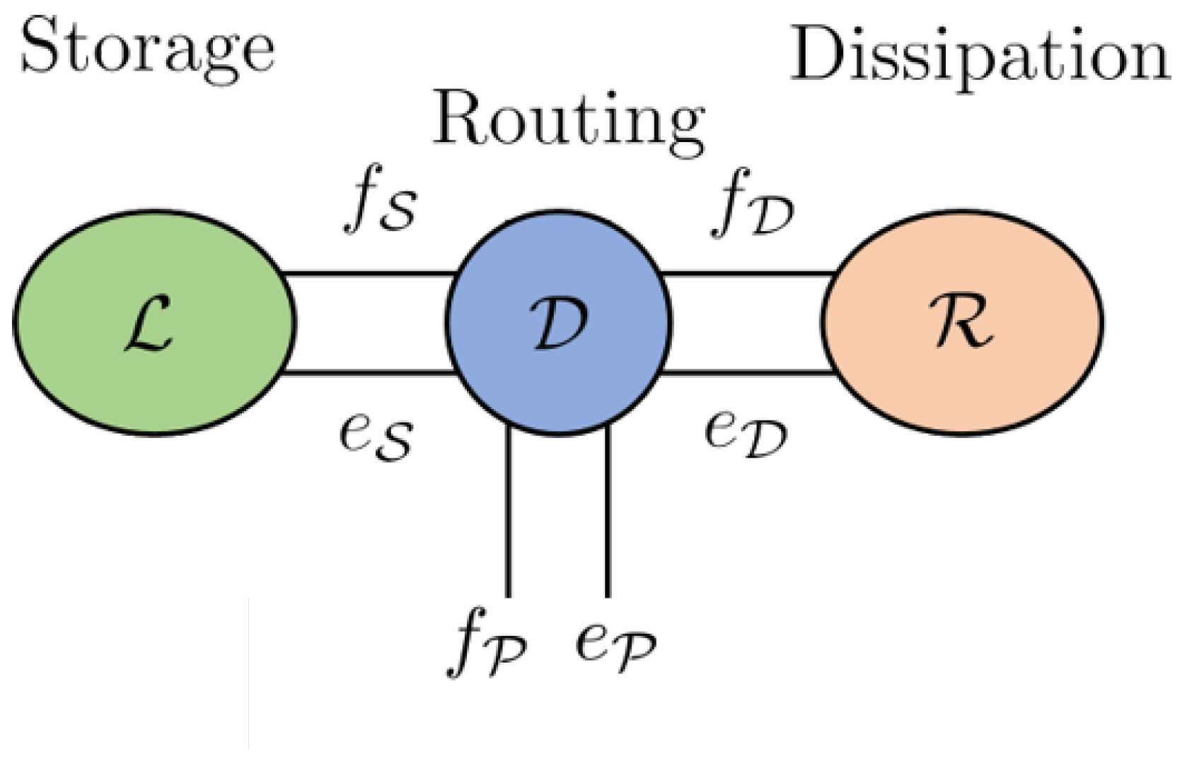
A key feature of a Dirac structure is the fact that the standard composition of two Dirac structures is again a Dirac structure. The implication of this statement is that any power-conserving interconnection of a Port–Hamiltonian system is also a Port–Hamiltonian system itself. This constitutes the foundational feature of the Port–Hamiltonian approach to modelling, simulation and control of complex physical systems. The intricate Dirac structure is the guide to the algebraic constraints of the interconnected system as well as its Casimir functions [23]. The Casimir functions are significant for the set-point regulation of Port–Hamiltonian systems. The framework of the Port–Hamiltonian approach allows for port-based modelling. Port-based modelling means that we are interconnecting many different elements through ports. Dirac structures are the tools used to connect multiple elements. These various elements are energy-storing elements, energy-dissipating elements and external elements that can supply energy. A diagram to demonstrate the connection structure is given in Figure 1 [23].

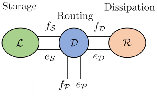
Figure 1. Energy storage, routing and dissipation.

3. Detailed Port–Hamiltonian Model of a Mechanical Ventilator

3.1. Description of the System

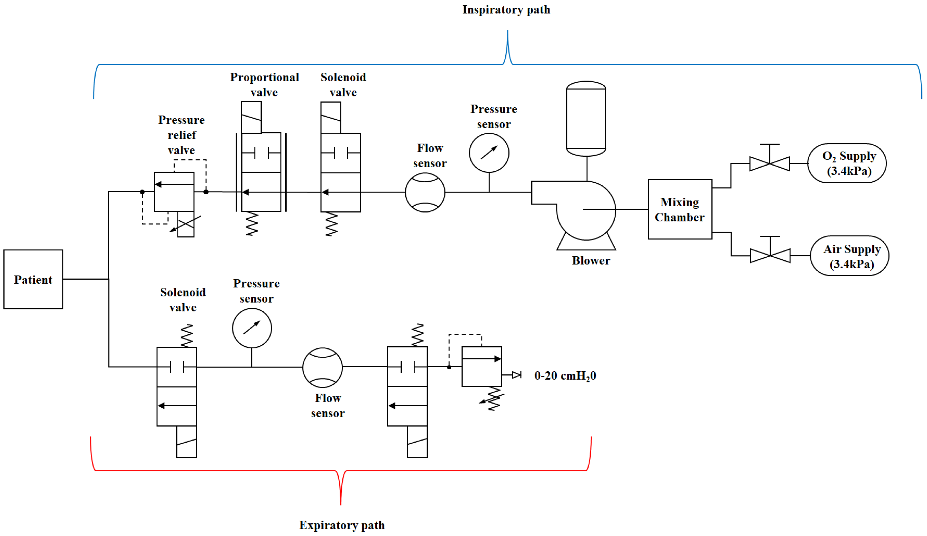
The overall mechanical ventilator system diagram is provided in Figure 2. The entire system consists of various subsystems. In this research work, the main subsystem that contributes to the flow of air and, consequently, the air pressure are discussed. Therefore, the following main subsystems will be discussed: the DC motor subsystem, the turbine pump/blower subsystem, the pump-shaft/impeller subsystem and the solenoid valve subsystem.

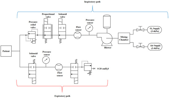
Figure 2. Schematic diagram of a mechanical ventilator.

3.2. Blower Model

In this section, the dynamical system model equations for the blower model are presented in the Port–Hamiltonian framework. The blower model comprises three sub-systems: namely, a DC motor that drives the blower-shaft/impeller, a blower-shaft/impeller that couples the DC motor to the fluid by using the rotational motion of the motor to accelerate the fluid, and finally, the fluid being driven.

From the Port–Hamiltonian perspective, the state vector ${\mathcal{X}}_b\in {\mathbb{R}}^4$ is given by:

$$\begin{array}{c}\hfill {\mathcal{X}}_b:={\left[\begin{array}{cccc}{p}_m,& {\varphi }_m,& P_b,& Q_b\end{array}\right]}^{\top },\end{array}$$

(4)

where $p_m\in {\mathbb{R}}^1$ and ${\varphi }_m\in {\mathbb{R}}^1$ are the angular momentum and magnetic flux of the DC motor, respectively, while $P_b\in {\mathbb{R}}^1$ and $Q_b\in {\mathbb{R}}^1$ are the pressure and flow rate of the blower, respectively.

The total energy of the blower is given by the Hamiltonian:

$$\begin{array}{ccc}\hfill {\mathcal{H}}_b\left[{\mathcal{X}}_b\right]& =& {\displaystyle \frac{1}{2}}\left({\displaystyle \frac{p_m^2}{I_m}}+{\displaystyle \frac{{\varphi }_m^2}{L_m}}+C_b{P}_b^2+I_b{Q}_b^2\right),\hfill \end{array}$$

(5)

where $I_m\in {\mathbb{R}}_{+}^1$ is the inertia and $L_m\in {\mathbb{R}}_{+}^1$ is the inductance of the DC motor, while $C_b\in {\mathbb{R}}_{+}^1$ and $I_b\in {\mathbb{R}}_{+}^1$ are the hydraulic capacitance and inertance of the air in the blower, respectively.

Thus, the Port–Hamiltonian model of a blower is given by

$$\begin{array}{ccc}\hfill {\dot{\mathcal{X}}}_b& =& \left({\mathcal{J}}_b-{\mathcal{R}}_b\right)\nabla {\mathcal{H}}_b\left[{\mathcal{X}}_b\right]+{\mathcal{G}}_b{u}_b,\hfill \end{array}$$

(6)

$$\begin{array}{ccc}\hfill {\mathcal{Y}}_b& =& {\mathcal{G}}_b^{*}\nabla {\mathcal{H}}_b\left[{\mathcal{X}}_b\right],\hfill \end{array}$$

(7)

where

$$\begin{array}{ccc}\hfill {\mathcal{J}}_b& :=& \left[\begin{array}{cccc}0& K_m& 0& -\left(K_o{p}_m\right)/I_m\\ -K_m& 0& 0& 0\\ 0& 0& 0& 1/\left(C_b{I}_b\right)\\ \left(K_o{p}_m\right)/I_m& 0& -1/\left(C_b{I}_b\right)& 0\end{array}\right]\in {\mathbb{R}}^{4\times 4},\hfill \\ \hfill {\mathcal{R}}_b& :=& \mathrm{diag}\left(\left[\begin{array}{cccc}{b}_m& R_m& 0& \left(R_b{p}_m\right)/\left(I_b{I}_m\right)\end{array}\right]\right)\in {\mathbb{R}}^{4\times 4},\hfill \\ \hfill \nabla {\mathcal{H}}_b\left[{\mathcal{X}}_b\right]& :=& \left[\begin{array}{cccc}{p}_m/I_m& {\varphi }_m/L_m& C_b{P}_b& I_b{Q}_b\end{array}\right]\in {\mathbb{R}}^{4\times 1},\hfill \\ \hfill {\mathcal{G}}_b& :=& \left[\begin{array}{ccc}1& 0& 0\\ 0& 0& 0\\ 0& -(1/C_b)& 0\\ 0& 0& (1/I_b)\end{array}\right]\in {\mathbb{R}}^{4\times 3},\hfill \\ \hfill u_b& :=& \left[\begin{array}{ccc}{V}_m& Q_{in}& P_{in}\end{array}\right]\in {\mathbb{R}}^{3\times 1},\hfill \end{array}$$

where $K_m\in {\mathbb{R}}_{+}^1$ is the motor torque constant, $b_m\in {\mathbb{R}}_{+}^1$ is the viscous damping, $R_m\in {\mathbb{R}}_{+}^1$ is the armature resistance, and $K_o\in {\mathbb{R}}_{+}^1$ is the motor’s angular momentum/pressure coupling constant. The inputs to the system are the DC motor voltage, the input volumetric flow rate and the pressure, which are given by $V\in {\mathbb{R}}^1$, $Q_{in}\in {\mathbb{R}}^1$ and $P_{in}\in {\mathbb{R}}^1$, respectively. One can easily show that ${\mathcal{J}}_m=-{\mathcal{J}}_m^{\top }$ and ${\mathcal{R}}_m={\mathcal{R}}_m^{\top }⪰0$.

Taking the time derivative of the Hamiltonian gives

$$\begin{array}{ccc}\hfill {\dot{\mathcal{H}}}_b\left[{\chi }_b\right]& =& u_b·{\mathcal{Y}}_b-\nabla {\mathcal{H}}_b\left[{\mathcal{X}}_b\right]·({\mathcal{R}}_b\nabla {\mathcal{H}}_b\left[{\mathcal{X}}_b\right]).\hfill \end{array}$$

(8)

This system has power and resistive ports.

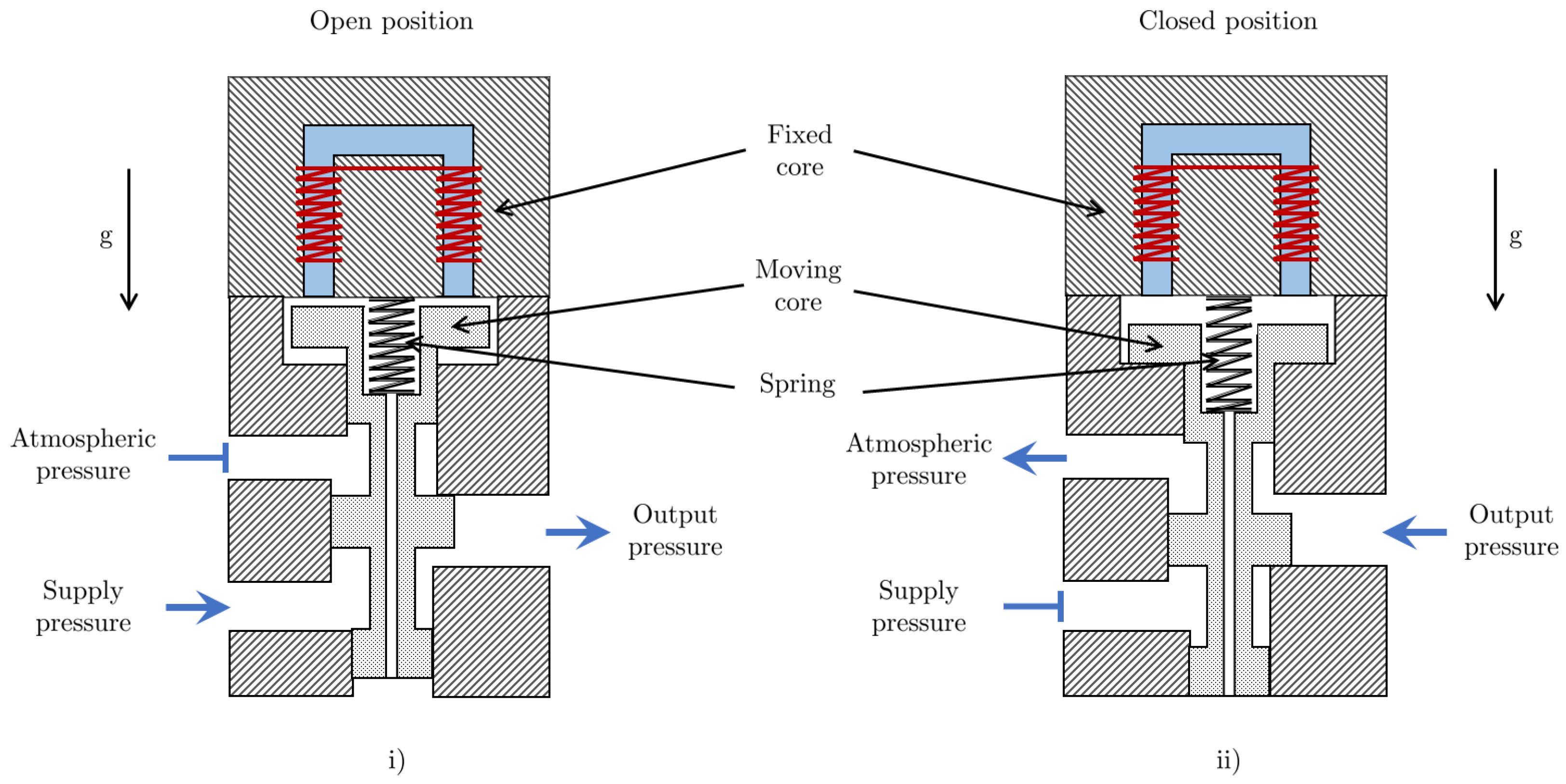
4. Solenoid Valve Subsystem

Figure 3 shows a solenoid valve in the open and closed positions. It is assumed that the air gaps are sufficiently small such that the effect of fringing of the magnetic flux is negligible. Consider a solenoid in which the permeability of the core and the length of the part of the magnetic circuit inside the core are denoted by ${\mu }_c\in {\mathbb{R}}_{+}^1$ and $l_c\in {\mathbb{R}}_{+}^1$, respectively. The equivalent length of the solenoid’s magnetic circuit $l_{eq}\left[·\right]:\mathbb{R}\to \mathbb{R}$ is dependent on the displacement of the spool $q_s\in \mathbb{R}$ and can be written as:

$$\begin{array}{ccc}\hfill l_{eq}\left[q_s\right]& =& l_c+{\displaystyle \frac{{\mu }_c}{{\mu }_0}}(q_{s_{\mathrm{tot}}}-q_s),\hfill \end{array}$$

(9)

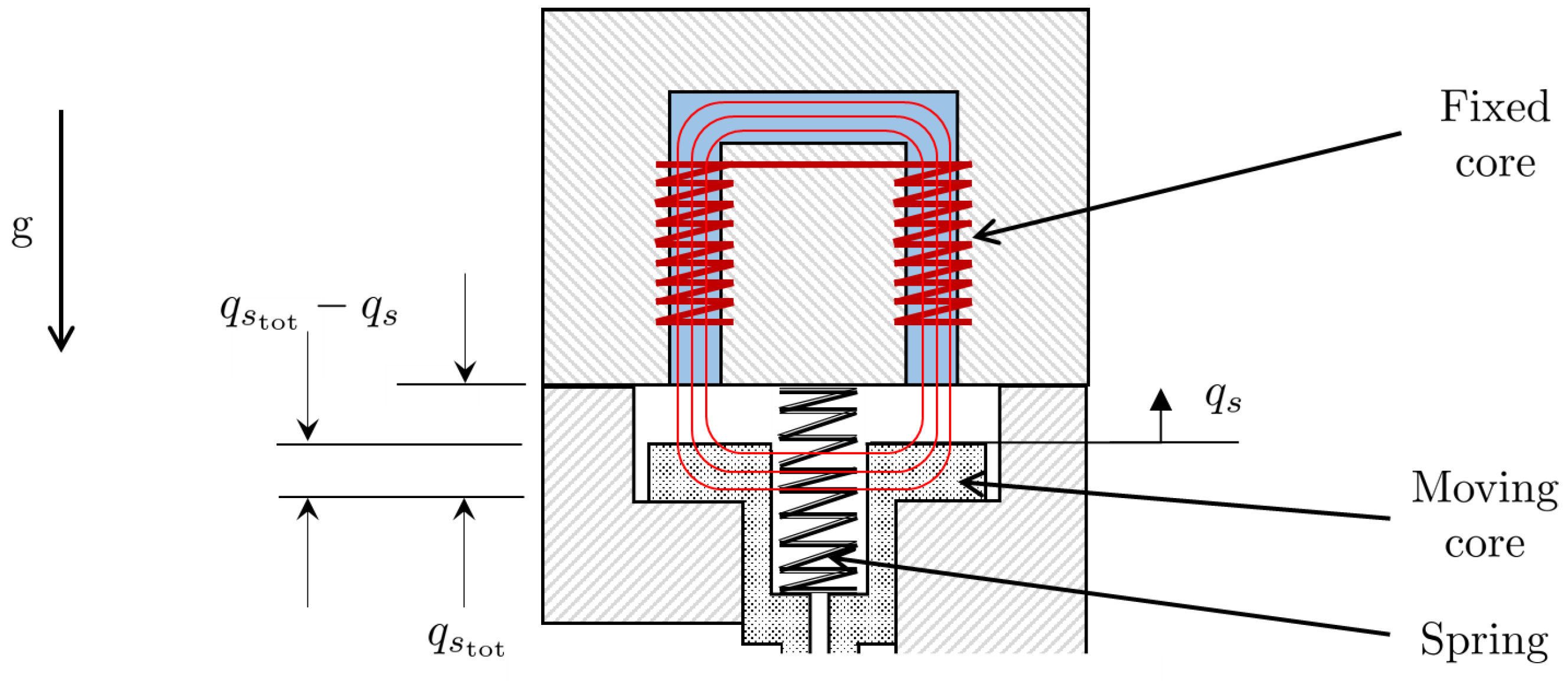
where ${\mu }_0\in {\mathbb{R}}_{+}^1$ is the permeability of air, and $q_{{\mathrm{s}}_{\mathrm{tot}}}\in {\mathbb{R}}_{+}^1$ is the total air gap. The solenoid coordinate system is represented in Figure 4. Thus, the inductance of the solenoid varies with displacement of the spool and, hence, can be expressed by the function $L_s\left[·\right]:\mathbb{R}\to \mathbb{R}$ given by:

$$\begin{array}{c}\hfill L_s\left[q_s\right]={\displaystyle \frac{N^2{A}_e{\mu }_c}{l_{eq}\left[q_s\right]}},\end{array}$$

(10)

where $N\in {\mathbb{R}}_{+}^1$ is the number of turns in the coil of the solenoid, and $A_e\in {\mathbb{R}}_{+}^1$ is the effective cross-sectional area of the path of the magnetic flux. The magnetic and mechanical subsystems in the solenoid valve are therefore coupled magnetically due to the dependence of the inductance on the displacement of the spool.

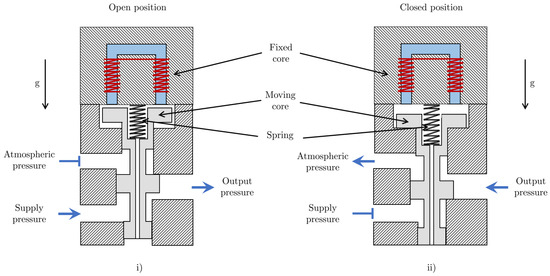
Figure 3. Diagram of a solenoid valve in (i) the open position, which allows fluid flow, and (ii) the closed position, which stops fluid flow.

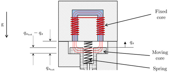
Figure 4. Solenoid coordinate system.

The total energy of the solenoid is given by the Hamiltonian ${\mathcal{H}}_s\left[·\right]:{\mathbb{R}}^3\to \mathbb{R}$, which is a function of the state vector ${\mathcal{X}}_s={\left[\begin{array}{ccc}{\varphi }_s,& p_s,& q_s\end{array}\right]}^{\top }\in {\mathbb{R}}^3$ and is expressed as the sum of the magnetic, kinetic and potential energies, which are denoted by ${\mathcal{H}}_{\mathrm{magnetic}}\left[{\varphi }_s,q_s\right]:{\mathbb{R}}^2\to \mathbb{R}$, ${\mathcal{H}}_{\mathrm{kinetic}}\left[p_s\right]:\mathbb{R}\to \mathbb{R}$ and ${\mathcal{H}}_{\mathrm{potential}}\left[q_s\right]:\mathbb{R}\to \mathbb{R}$, respectively. Thus,

$$\begin{array}{c}\hfill {\mathcal{H}}_s\left[{\mathcal{X}}_s\right]={\mathcal{H}}_{\mathrm{magnetic}}\left[{\varphi }_s,q_s\right]+{\mathcal{H}}_{\mathrm{kinetic}}\left[p_s\right]+{\mathcal{H}}_{\mathrm{potential}}\left[q_s\right],\end{array}$$

(11)

given a magnetic flux ${\varphi }_s\in \mathbb{R}$.

Assuming that the pretension of the spring is set to $q_0\in \mathbb{R}$, the Hamiltonian is

$$\begin{array}{c}\hfill {\mathcal{H}}_s\left[{\mathcal{X}}_s\right]={\displaystyle \frac{1}{2}}\left({\displaystyle \frac{{\varphi }_s^2}{L\left[q_s\right]}}+{\displaystyle \frac{p_s^2}{m_s}}+k_s{(q_s+q_{s_0})}^2\right)+m_s{q}_{s}g,\end{array}$$

(12)

where $p_s\in \mathbb{R}$ is the momentum of the spool, $m_s\in {\mathbb{R}}_{+}^1$ is the mass of the spool, $k_s\in {\mathbb{R}}_{+}^1$ is the spring stiffness, and $g\in {\mathbb{R}}_{+}^1$ is the acceleration due to gravity.

Hence, the solenoid’s state and output dynamics are expressed in Port–Hamiltonian form in Equations (13) and (14), respectively:

$$\begin{array}{ccc}\hfill {\dot{\mathcal{X}}}_s& =& \left({\mathcal{J}}_s-{\mathcal{R}}_s\right)\nabla {\mathcal{H}}_s\left[{\mathcal{X}}_s\right]+{\mathcal{G}}_s{u}_s,\hfill \end{array}$$

(13)

$$\begin{array}{ccc}\hfill {\mathcal{Y}}_s& =& {\mathcal{G}}_s^{*}{u}_s,\hfill \end{array}$$

(14)

where

$$\begin{array}{ccc}\hfill {\mathcal{J}}_s& =& \left[\begin{array}{ccc}0& 0& 0\\ 0& 0& -1\\ 0& 1& 0\end{array}\right],{\mathcal{R}}_s=\left[\begin{array}{ccc}{R}_s& 0& 0\\ 0& b_s& 0\\ 0& 0& 0\end{array}\right],{\mathcal{G}}_s=\left[\begin{array}{cc}1& 0\\ 0& 0& 0\\ 0& (A_{s_1}-A_{s_2})& (A_{s_3}-A_{s_4})\end{array}\right],\hfill \\ \hfill {\mathcal{G}}_s^{*}& =& {\mathcal{G}}_s^{\top },u_s=\left[\begin{array}{c}{V}_s\\ p_s\end{array}\right]\mathrm{and}\nabla {\mathcal{H}}_s\left[{\mathcal{X}}_s\right]=\left[\begin{array}{c}{\displaystyle \frac{{\varphi }_s}{A_e{N}^2{\mu }_c}}\left(l_c-{\displaystyle \frac{{\mu }_c(q_s-q_{s_{\mathrm{tot}}})}{{\mu }_0}}\right)\\ {\displaystyle \frac{p_s}{m_s}}\\ {\displaystyle \frac{A_e{N}^2{\mu }_c^2{\mu }_0}{{\left({\mu }_0{l}_c-{\mu }_c(q_s-q_{s_{\mathrm{tot}}})\right)}^2}}+k_s(q_s+q_{s_0})+m_{s}g\end{array}\right],\hfill \end{array}$$

where $R_s\in {\mathbb{R}}_{+}^1$ is the resistance of the coil, $b_s\in {\mathbb{R}}_{+}^1$ is the viscous damping acting on the spool, and ∇ is the gradient operator. $A_{s_1},A_{s_2}\in {\mathbb{R}}_{+}^1$ are the various cross-sectional areas of the surfaces of the spool, and the input vector $u_s\in {\mathbb{R}}^2$ consists of the input voltage $V_s\in {\mathbb{R}}^1$ and the supply pressure $p_s\in {\mathbb{R}}^1$. It can be seen that ${\mathcal{J}}_s=-{\mathcal{J}}_s^{\top }\in {\mathbb{R}}^{3\times 3}$ possesses skew symmetry, while ${\mathcal{R}}_s={\mathcal{R}}_s^{\top }\in {\mathbb{R}}^{3\times 3}$ is positive semi-definite.

Taking the time derivative of the Hamiltonian gives:

$$\begin{array}{ccc}\hfill {\dot{\mathcal{H}}}_s\left[{\chi }_s\right]& =& u_s·{\mathcal{Y}}_s-\nabla {\mathcal{H}}_s\left[{\mathcal{X}}_s\right]·({\mathcal{R}}_s\nabla {\mathcal{H}}_s\left[{\mathcal{X}}_s\right]).\hfill \end{array}$$

(15)

This system has power and resistive ports.

4.1. Pipe Model

In this section, a Port–Hamiltonian model of a single pipe segment is developed. The basis of these developments is the Navier–Stokes equations for one-dimensional non-stationary flow of gas in a pipe. The following assumptions are taken for the sake of model simplification [24,25]:

• The pipe is taken as rigid (the cross-section does not expand as a result of fluid flow).
• Frictional and gravitational effects are neglected (this will be relaxed in future works in this research area).
• The model parameters of the gas remain constant along the pipe cross-section but vary in time along the pipe length. Thus, they can be averaged about the cross-section, and thus, the gas flow is one-dimensional.
• The temperatures of the pipe walls are assumed to be constant and equal to the ambient room temperature. Hence, temperature effects are ignored.

Taking into account these assumptions, the coordinate system attached to a segment of pipe is illustrated in Figure 5. Thus, for a given time interval $t_s\le t<t_f$ with start time $t_s$ and finish time $t_f$, the length-normalized one-dimensional Euler equations for gas with a density $\rho (t,z):(t_s,t_f]\times (0,\ell )\to {\mathbb{R}}^1$ flowing at a velocity $\nu (t,z):(t_s,t_f]\times (0,\ell )\to {\mathbb{R}}^1$ through a pipe of length $\ell \in {\mathbb{R}}_{+}^1$ and cross-sectional area $A_p\in {\mathbb{R}}_{+}^1$ are given by:

$$\begin{array}{cc}\hfill & {\partial }_t\left(\rho A_p\right)+{\partial }_z\left(\rho A_p\nu \right)=0,\hfill \end{array}$$

(16)

$$\begin{array}{cc}\hfill & {\partial }_t\left(\rho A_p\nu \right)+{\partial }_z(\rho A_p{\nu }^2+p{A}_p)=0,\hfill \end{array}$$

(17)

where $p(t,z):(t_s,t_f]\times (0,\ell )\to {\mathbb{R}}^1$ is the pressure, and ${\partial }_i:=\partial /{\partial }_i$ is the partial derivative with respect to the temporal and spatial variables given by the subscripts $i\in \left\{t,z\right\}$.

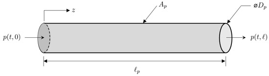
Figure 5. Pipe segment coordinate system.

Port–Hamiltonian Formulation of Pipe-Flow Model

The fluid dynamics can be written in terms of mass per unit length, i.e., $\varrho :=\rho A_p$, as well as the fluid momentum, $m:=\varrho \nu$. Thus, Equations (16) and (17) can be expressed as

$$\begin{array}{ccc}\hfill & \hfill & \hfill {\partial }_t\varrho =-{\partial }_{z}m,\end{array}$$

(18)

$$\begin{array}{ccc}\hfill & \hfill & \hfill {\partial }_{t}m=-{\partial }_z\left({\displaystyle \frac{m^2}{\varrho }}+p{A}_p\right),\end{array}$$

(19)

Defining the state vector of the gas flow through a pipe segment as ${\chi }_p:=\left[\begin{array}{c}\varrho \\ m\end{array}\right]$, the energy of the gas can be expressed in the form of a Hamiltonian ${\mathcal{H}}_p\left[{\chi }_p\right]:{\mathbb{R}}^2\to {\mathbb{R}}^1$ given by

$$\begin{array}{c}\hfill {\mathcal{H}}_p\left[{\chi }_p\right]={\int }_0^{\ell }{H}_p\left[{\chi }_p\right]\mathrm{d}x={\int }_0^{\ell }\left({\displaystyle \frac{m^2}{2\varrho }}+\varrho U\left[\varrho /A_p\right]\right)\mathrm{d}x,\end{array}$$

(20)

where $H_p\left[·\right]:{\mathbb{R}}^2\to {\mathbb{R}}^1$ is the Hamiltonian density, and $U\left[·\right]:{\mathbb{R}}^1\to {\mathbb{R}}^1$ is the internal energy of the gas, which, in the case of an isentropic fluid, can be expressed as a function of density.

The Port–Hamiltonian dynamics take the following form:

$$\begin{array}{c}\hfill {\partial }_t{\chi }_p=\mathcal{J}\left[{\chi }_p\right]{\delta }_{{\chi }_p}{\mathcal{H}}_p\left[{\chi }_p\right],\end{array}$$

(21)

where $\mathcal{J}\left[{\chi }_p\right]$, which is the formally skew-symmetric operator, and ${\delta }_{{\chi }_p}\mathcal{H}\left[{\chi }_p\right]$, which is the variational derivative of the Hamiltonian density, are expressed as

$$\begin{array}{c}\hfill \mathcal{J}\left[{\chi }_p\right]=-\left[\begin{array}{cc}0& {\partial }_z\\ {\partial }_z& 0\end{array}\right]\mathrm{and}{\delta }_{{\chi }_p}{\mathcal{H}}_p\left[{\chi }_p\right]=\left[\begin{array}{c}h-{\displaystyle \frac{m^2}{2{\varrho }^2}}\\ {\displaystyle \frac{m}{\varrho }}\end{array}\right],\end{array}$$

(22)

where h is the enthalpy, and $\mathcal{J}\left[{\chi }_p\right]$ is a formally skew-symmetric operator.

The rate of change of the Hamiltonian can be found as

$$\begin{array}{c}\hfill {\dot{\mathcal{H}}}_p={\mathbf{u}}_p^{\top }{\mathbf{y}}_p,\end{array}$$

(23)

where

$$\begin{array}{c}\hfill {\mathbf{u}}_p=W_B{R}_{\mathrm{ext}}\left[\begin{array}{c}{\left.{\delta }_{{\chi }_p}{\mathcal{H}}_p\right|}_0\\ {\left.{\delta }_{{\chi }_p}{\mathcal{H}}_p\right|}_{\ell }\end{array}\right]\mathrm{and}{\mathbf{y}}_p=W_C{R}_{\mathrm{ext}}\left[\begin{array}{c}{\left.{\delta }_{{\chi }_p}{\mathcal{H}}_p\right|}_0\\ {\left.{\delta }_{{\chi }_p}{\mathcal{H}}_p\right|}_{\ell }\end{array}\right],\end{array}$$

(24)

with components given by

$$\begin{array}{c}\hfill W_B={\displaystyle \frac{1}{\sqrt{2}}}\left[\begin{array}{cccc}1& 0& 0& 1\\ 0& -1& 1& 0\end{array}\right],W_C={\displaystyle \frac{1}{\sqrt{2}}}\left[\begin{array}{cccc}0& 1& 1& 0\\ 1& 0& 0& -1\end{array}\right],R_{\mathrm{ext}}={\displaystyle \frac{1}{\sqrt{2}}}\left[\begin{array}{cccc}0& -1& 0& 1\\ -1& 0& 1& 0\\ 1& 0& 1& 0\\ 0& 1& 0& 1\end{array}\right],\end{array}$$

and

$$\begin{array}{c}\hfill \left[\begin{array}{c}{\left.{\delta }_{{\chi }_p}{\mathcal{H}}_p\right|}_0\\ {\left.{\delta }_{{\chi }_p}{\mathcal{H}}_p\right|}_{\ell }\end{array}\right]=\left[\begin{array}{c}{\left.\left(h-{\displaystyle \frac{m^2}{2{\varrho }^2}}\right)\right|}_0\\ {\left.\left({\displaystyle \frac{m}{\varrho }}\right)\right|}_0\\ {\left.\left(h-{\displaystyle \frac{m^2}{2{\varrho }^2}}\right)\right|}_{\ell }\\ {\left.\left({\displaystyle \frac{m}{\varrho }}\right)\right|}_{\ell }\end{array}\right].\end{array}$$

Expanding ${\mathbf{u}}_p$ and ${\mathbf{y}}_p$ gives

$$\begin{array}{c}\hfill {\mathbf{u}}_p=\left[\begin{array}{c}{\left.\left({\displaystyle \frac{m}{\varrho }}\right)\right|}_{\ell }\\ {\left.\left(h-{\displaystyle \frac{m^2}{2{\varrho }^2}}\right)\right|}_0\end{array}\right]\mathrm{and}{\mathbf{y}}_p=\left[\begin{array}{c}{\left.\left(h-{\displaystyle \frac{m^2}{2{\varrho }^2}}\right)\right|}_{\ell }\\ -{\left.\left({\displaystyle \frac{m}{\varrho }}\right)\right|}_0\end{array}\right].\end{array}$$

(25)

Thus, the rate of change of the Hamiltonian is

$$\begin{array}{c}\hfill {\dot{\mathcal{H}}}_p={\left.\left(h-{\displaystyle \frac{m^2}{2{\varrho }^2}}\right)\right|}_{\ell }{\left.\left({\displaystyle \frac{m}{\varrho }}\right)\right|}_{\ell }-{\left.\left({\displaystyle \frac{m}{\varrho }}\right)\right|}_0{\left.\left(h-{\displaystyle \frac{m^2}{2{\varrho }^2}}\right)\right|}_0.\end{array}$$

(26)

4.2. Electric Circuit Model of the Lung

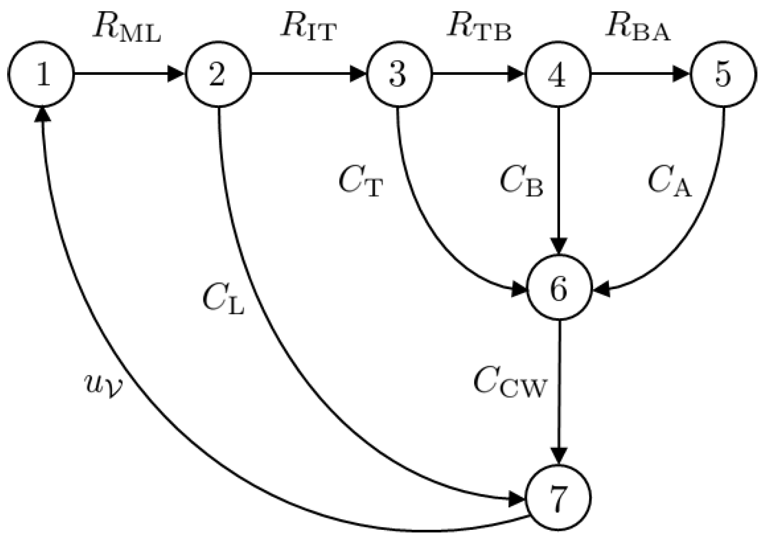
The Port–Hamiltonian formulation for nonlinear electric circuits is presented in this section. Since the main focus of this article is a mechanical ventilator model, the lung model is simplified by considering an electric circuit analogy. The model under consideration is that of a fully sedated patient who relies completely on the mechanical ventilator to breathe. The circuit model is shown in Figure 6. The circuit can be represented in the form of a network graph using graph theory. The graph of the circuit given in Figure 6 is given in Figure 7. The model has $n=\left|\mathcal{V}\right|=7$ vertices.

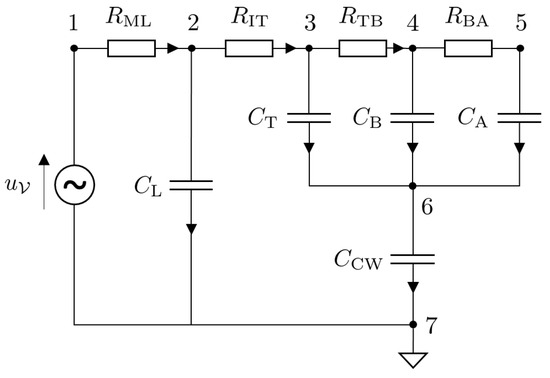
Figure 6. Circuit diagram of an electric model of a lung of a fully sedated patient [26].

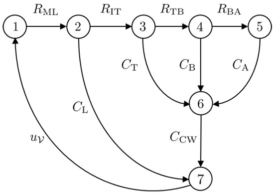
Figure 7. The graph associated with the circuit diagram given in Figure 6.

The complete graph of the circuit, $A_0$, is

$${\mathcal{A}}_0=\begin{array}{ccccccccccc}\begin{array}{c}\hfill R_{ML}\end{array}& \begin{array}{c}{R}_{IT}\end{array}& \begin{array}{c}{R}_{TB}\end{array}& \begin{array}{c}{R}_{BA}\hfill \end{array}& \begin{array}{c}{C}_T\end{array}& \begin{array}{c}{C}_B\end{array}& \begin{array}{c}{C}_A\end{array}& \begin{array}{c}{C}_L\end{array}& \begin{array}{c}{C}_{CW}\end{array}& \begin{array}{c}{u}_{\mathcal{V}}\end{array}& \begin{array}{c}\end{array}\\ [\begin{array}{c}1\\ -1\\ 0\\ 0\\ 0\\ 0\\ 0\end{array}& \begin{array}{c}0\\ 1\\ -1\\ 0\\ 0\\ 0\\ 0\end{array}& \begin{array}{c}0\\ 0\\ 1\\ -1\\ 0\\ 0\\ 0\end{array}& \begin{array}{c}0\\ 0\\ 0\\ 1\\ -1\\ 0\\ 0\end{array}|& \begin{array}{c}0\\ 0\\ 1\\ 0\\ 0\\ -1\\ 0\end{array}& \begin{array}{c}0\\ 0\\ 0\\ 1\\ 0\\ -1\\ 0\end{array}& \begin{array}{c}0\\ 0\\ 0\\ 0\\ 1\\ -1\\ 0\end{array}& \begin{array}{c}0\\ 1\\ 0\\ 0\\ 0\\ 0\\ -1\end{array}& \begin{array}{c}0\\ 0\\ 0\\ 0\\ 0\\ 1\\ -1\end{array}& | \begin{array}{c}-1\\ 0\\ 0\\ 0\\ 0\\ 0\\ 1\end{array}]& \begin{array}{c}1\\ 2\\ 3\\ 4\\ 5\\ 6\\ 7\end{array}\end{array}.$$

(27)

The ventilator input voltage is represented as a source $\mathcal{S}=({\mathcal{D}}_{\mathcal{S}},{\mathcal{L}}_{\mathcal{S}},{\mathcal{R}}_{\mathcal{S}})$. The set of sources is $\mathcal{S}=\left\{v_7\right\}$, and the dimension of the source is $\left|\mathcal{S}\right|=1$. The circuit also consists of $m_{\mathcal{C}}=5$ capacitors (storage elements) that are represented as ${\mathcal{C}}_i=({\mathcal{D}}_{{\mathcal{C}}_i},{\mathcal{L}}_{{\mathcal{C}}_i},{\mathcal{R}}_{{\mathcal{C}}_i})$, where the $i\mathrm{th}$ index used to distinguish between the components is $i=\left\{\begin{array}{ccccc}{C}_{\mathrm{L}},& C_{\mathrm{T}},& C_{\mathrm{B}},& C_{\mathrm{A}},& C_{\mathrm{CW}}\end{array}\right\}$. Furthermore there are $m_{\mathcal{R}}=4$ resistors (dissipative elements) that are represented as ${\mathcal{R}}_i=({\mathcal{D}}_{{\mathcal{R}}_i},{\mathcal{L}}_{{\mathcal{R}}_i},{\mathcal{R}}_{{\mathcal{R}}_i})$, where the $i\mathrm{th}$ index is given by $i=\left\{\begin{array}{cccc}{R}_{\mathrm{ML}},& R_{\mathrm{IT}},& R_{\mathrm{TB}},& R_{\mathrm{BA}}\end{array}\right\}$.

Selecting node 7 as the ground, the reduced incidence matrix, $\mathcal{A}$, is given by

$$A=[\begin{array}{ccc}{A}_{\mathcal{R}}& A_{\mathcal{C}}& A_{\mathcal{S}}\end{array}]=\begin{array}{ccc}\left(\begin{array}{c}1\\ -1\\ 0\\ 0\\ 0\\ 0\end{array}\begin{array}{c}0\\ 1\\ -1\\ 0\\ 0\\ 0\end{array}\begin{array}{c}0\\ 0\\ 1\\ -1\\ 0\\ 0\end{array}\begin{array}{c}0\\ 0\\ 0\\ 1\\ -1\\ 0\end{array}\right|& \begin{array}{c}0\\ 0\\ 1\\ 0\\ 0\\ -1\end{array}\begin{array}{c}0\\ 0\\ 0\\ 1\\ 0\\ -1\end{array}\begin{array}{c}0\\ 0\\ 0\\ 0\\ 1\\ -1\end{array}\begin{array}{c}0\\ 1\\ 0\\ 0\\ 0\\ 0\end{array}\begin{array}{c}0\\ 0\\ 0\\ 0\\ 0\\ 1\end{array}& \left|\begin{array}{c}-1\\ 0\\ 0\\ 0\\ 0\\ 0\end{array}\right)\\ ⏟& ⏟& ⏟\\ A_{\mathcal{R}}& A_{\mathcal{C}}& A_{\mathcal{S}}\end{array},$$

(28)

where the dimensions of the components of $\mathcal{A}$ are $dim\left(A_{\mathcal{R}}\right)=(n-|S\left|\right)\times m_{\mathcal{R}}=6\times 4$, $dim\left(A_{\mathcal{C}}\right)=(n-|S\left|\right)\times m_{\mathcal{C}}=6\times 5$ and $dim\left(A_{\mathcal{S}}\right)=(n-|S\left|\right)\times m_{\mathcal{S}}=6\times 1$.

The total energy of the circuit is given by the Hamiltonian

$$\begin{array}{c}\hfill {\mathcal{H}}_C=\sum _{\forall i}{\mathcal{H}}_{C_i}\left(q_{C_i}\right)={\displaystyle \frac{1}{2}}\sum _{\forall i}{\displaystyle \frac{q_{C_i}}{C_i}},\end{array}$$

(29)

where $q_{C_i}\in {\mathbb{R}}^1$ is the charge of the $i\mathrm{th}$ capacitor for $i=\left\{\begin{array}{ccccc}{C}_{\mathrm{L}},& C_{\mathrm{T}},& C_{\mathrm{B}},& C_{\mathrm{A}},& C_{\mathrm{CW}}\end{array}\right\}$. Thus,

$$\begin{array}{c}\hfill \left[\begin{array}{cccc}\mathbb{I}& A_{\mathcal{C}}& A_{\mathcal{R}}& A_{\mathcal{S}}\\ \mathbb{O}& \mathbb{O}& \mathbb{O}& \mathbb{O}\\ \mathbb{O}& \mathbb{O}& \mathbb{O}& \mathbb{O}\\ \mathbb{O}& \mathbb{O}& \mathbb{O}& \mathbb{O}\end{array}\right]\left(\begin{array}{c}-{\displaystyle \frac{d}{dt}}q\\ -{\displaystyle \frac{d}{dt}}{q}_{\mathcal{C}}\\ -i_{\mathcal{R}}\\ -i_{\mathcal{S}}\end{array}\right)+\left[\begin{array}{cccc}\mathbb{O}& \mathbb{O}& \mathbb{O}& \mathbb{O}\\ -A_{\mathcal{R}}^{\top }& \mathbb{O}& \mathbb{I}& \mathbb{O}\\ -A_{\mathcal{C}}^{\top }& \mathbb{I}& \mathbb{O}& \mathbb{O}\\ -A_{\mathcal{S}}^{\top }& \mathbb{O}& \mathbb{O}& \mathbb{I}\end{array}\right]\left(\begin{array}{c}\varphi \\ u_{\mathcal{C}}\\ u_{\mathcal{R}}\\ u_{\mathcal{S}}\end{array}\right)=\mathbb{O},\end{array}$$

(30)

where $\mathbb{I}$ and $\mathbb{O}$ are appropriately sized identity and zero matrices, respectively, $q=0$, and $\varphi$ is the node potential. Expanding Equation (30) gives

$$\begin{array}{c}\hfill A_{\mathcal{C}}{\displaystyle \frac{d}{dt}}{q}_{\mathcal{C}}+A_{\mathcal{R}}\left(A_{\mathcal{R}}^{\top }\varphi \right)+A_{\mathcal{S}}{i}_{\mathcal{S}}=0,\end{array}$$

(31)

$$\begin{array}{c}\hfill -A_{\mathcal{C}}^{\top }\varphi +u_{\mathcal{C}}=0,\end{array}$$

(32)

$$\begin{array}{c}\hfill -A_{\mathcal{S}}^{\top }\varphi +u_{\mathcal{S}}=0.\end{array}$$

(33)

The Dirac structure is given by the set with the following attributes for $\left(\mathcal{D},\mathcal{L},\mathcal{R}\right)$:

$$\begin{array}{c}\hfill \left(\begin{array}{cccccccc}-{\displaystyle \frac{d}{dt}}q,& -{\displaystyle \frac{d}{dt}}{q}_{\mathcal{C}},& -i_{\mathcal{R}},& -i_{\mathcal{S}},& \varphi ,& u_{\mathcal{C}},& u_{\mathcal{R}},& u_{\mathcal{S}}\end{array}\right)\in \mathcal{D},\end{array}$$

(34)

$$\begin{array}{c}\hfill \left(\begin{array}{cccc}q,& q_{\mathcal{C}},& \varphi ,& u_{\mathcal{C}}\end{array}\right)\in \mathcal{L},\end{array}$$

(35)

$$\begin{array}{c}\hfill \left(\begin{array}{cc}-i_{\mathcal{R}},& e_{\mathcal{R}}\end{array}\right)\in \mathcal{R}.\end{array}$$

(36)

5. Model Network Topology

Definition 11.

(Directed graph) [27]: A directed graph $\mathcal{G}$ denotes the pair $(\mathcal{V},\mathcal{A})$, where $\mathcal{V}\left(\mathcal{D}\right)$ and $\mathcal{A}\left(\mathcal{D}\right)$ denote the set of vertices and arcs, respectively. An arc is a distinct ordered-pair of vertices.

The directed graph of a mechanical ventilator model is composed of the disjoint union of the vertices associated with the patient as well as the inspiratory and expiratory limbs of the ventilator, which are given by $v_O,{\mathcal{V}}_I$ and ${\mathcal{V}}_E$, respectively. Similarly, the patient, inspiratory and expiratory arcs are given by $a_O,{\mathcal{A}}_I$ and ${\mathcal{A}}_E$, respectively. Each arc and vertex can further be subdivided into those associated with the blowers, valves, pipes and electric circuits present in the mechanical ventilator. Thus, the totality of vertices and arcs is given by

$$\begin{array}{c}\hfill \mathcal{V}\left(\mathcal{D}\right)=\left\{v_O\right\}\cup {\mathcal{V}}_I\cup {\mathcal{V}}_E=\left\{v_O\right\}\cup ({\mathcal{V}}_{I_b}\cup {\mathcal{V}}_{I_v}\cup {\mathcal{V}}_{I_p}\cup {\mathcal{V}}_{I_e})\cup ({\mathcal{V}}_{E_b}\cup {\mathcal{V}}_{E_v}\cup {\mathcal{V}}_{E_p}\cup {\mathcal{V}}_{E_e})\end{array}$$

and

$$\begin{array}{c}\hfill \mathcal{A}\left(\mathcal{D}\right)=\left\{a_O\right\}\cup {\mathcal{A}}_I\cup {\mathcal{A}}_E=\left\{a_O\right\}\cup ({\mathcal{A}}_{I_b}\cup {\mathcal{A}}_{I_v}\cup {\mathcal{A}}_{I_p}\cup {\mathcal{A}}_{I_e})\cup ({\mathcal{A}}_{E_b}\cup {\mathcal{A}}_{E_v}\cup {\mathcal{A}}_{E_p}\cup {\mathcal{A}}_{E_e}),\end{array}$$

respectively, where the subscripts $i\in \left\{O,p,b,v,p,e\right\}$ are used to indicate the patient, blowers, valves, pipes and electric circuit components, respectively.

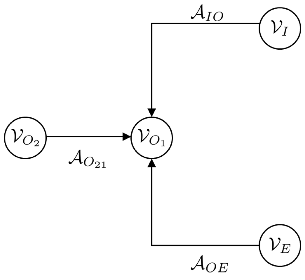
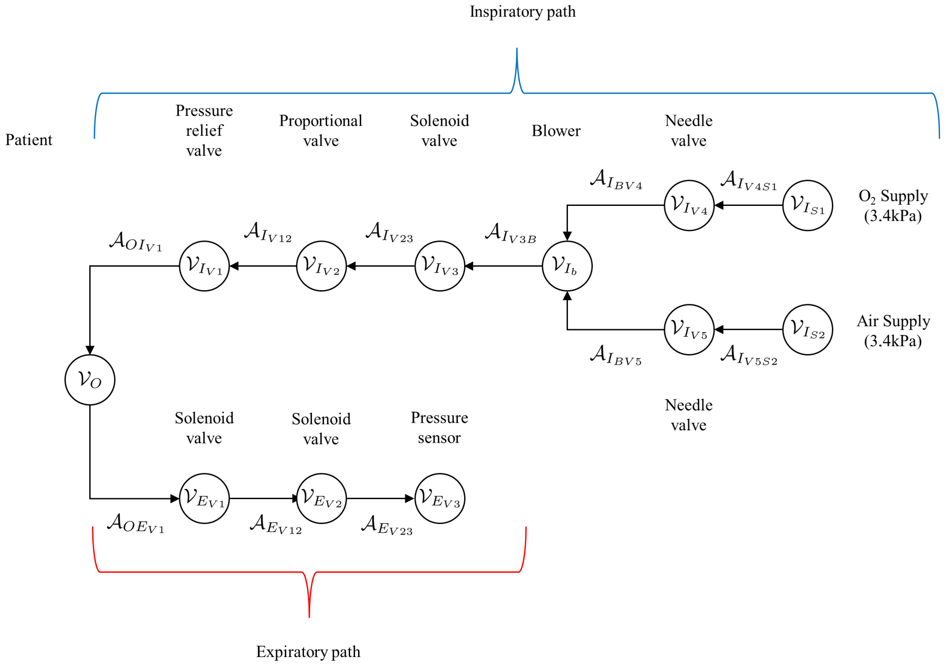
A simplified graph of the mechanical ventilator shown in Figure 2 is given in Figure 8. This simplified graph indicates the elements belonging to the patient, as well as the inspiratory arcs and vertices belonging to the mechanical ventilator. The arcs belonging to the patient are denoted by ${\mathcal{A}}_{O_{21}}\in {\mathcal{A}}_O$, while the vertices are denoted by $\left\{{\mathcal{V}}_{O_1},{\mathcal{V}}_{O_2}\right\}\in {\mathcal{V}}_O$. The elements of the inspiratory and expiratory arcs and vertices, given by ${\mathcal{V}}_I,{\mathcal{V}}_E$ and ${\mathcal{A}}_{IO},{\mathcal{A}}_{OE}$, respectively. A more detailed representation of the graph of the mechanical ventilator in Figure 8 is given in Figure 9.

Figure 8. Simplified graph of the mechanical ventilator given in Figure 2 indicating the elements belonging to the patient, given by the arcs ${\mathcal{A}}_{O_{21}}\in {\mathcal{A}}_O$ and vertices $\left\{{\mathcal{V}}_{O_1},{\mathcal{V}}_{O_2}\right\}\in {\mathcal{V}}_O$, as well as elements of the inspiratory and expiratory arcs and vertices, given by ${\mathcal{V}}_I,{\mathcal{V}}_E$ and ${\mathcal{A}}_{IO},{\mathcal{A}}_{OE}$, respectively.

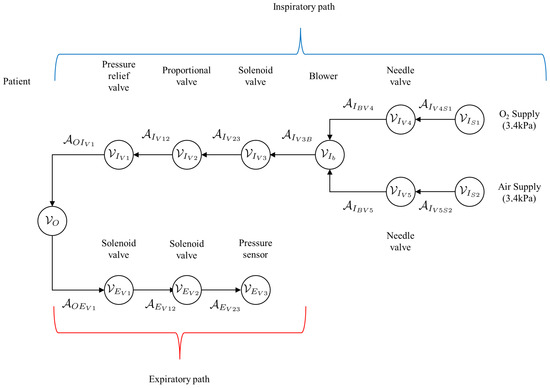
Figure 9. Detailed graph of the mechanical ventilator given in Figure 8 indicating the patient vertex ${\mathcal{V}}_O$ as well as the arcs and vertices along the inspiratory and expiratory paths.

Figure 9 shows a detailed graph of the mechanical ventilator given in Figure 2 that indicates the patient vertex ${\mathcal{V}}_O$ and the arcs and vertices along the inspiratory path, given by

$$\begin{array}{c}\hfill {\mathcal{A}}_I:=\left\{{\mathcal{A}}_{I_{V12}},{\mathcal{A}}_{I_{V23}},{\mathcal{A}}_{I_{V3B}},{\mathcal{A}}_{I_{V23}},{\mathcal{A}}_{I_{BV4}},{\mathcal{A}}_{I_{V4S1}},{\mathcal{A}}_{I_{BV5}},{\mathcal{A}}_{I_{V5S2}}\right\}\end{array}$$

and

$$\begin{array}{c}\hfill {\mathcal{V}}_I:=\left\{{\mathcal{V}}_{I_{V1}},{\mathcal{V}}_{I_{V2}},{\mathcal{V}}_{I_{V3}},{\mathcal{V}}_{I_B},{\mathcal{V}}_{I_{V4}},{\mathcal{V}}_{I_{S1}},{\mathcal{V}}_{I_{V5}},{\mathcal{V}}_{I_{S2}}\right\},\end{array}$$

respectively, as well as the arcs and vertices along the expiratory path, given by

$$\begin{array}{c}\hfill {\mathcal{A}}_E:=\left\{{\mathcal{A}}_{O{E}_{V1}},{\mathcal{A}}_{E_{V12}},{\mathcal{A}}_{E_{V23}}\right\}\mathrm{and}{\mathcal{V}}_E:=\left\{{\mathcal{V}}_{E_{V1}},{\mathcal{V}}_{E_{V2}},{\mathcal{V}}_{E_{V3}}\right\},\end{array}$$

respectively.

6. Model Interconnection/Coupling Conditions

In this section, the coupling conditions of the Port–Hamiltonian network model of the mechanical ventilator are given. The types of interconnections occurring in this model are given below:

• Pump-to-pipe interconnection: The pressure and flow rate of the fluid exiting the pump, $P_b$ and $Q_b$, respectively, are equal to the pressure and flow rate at the inlet of the pipe, given by $p\left(0\right)$ and $m\left(0\right)$, respectively. Thus,

  $$\begin{array}{c}\hfill P_b=p_0\mathrm{and}{Q}_b=m\left(0\right).\end{array}$$
• Pipe-to-valve interconnection: The pressure and flow rate of the fluid entering/exiting a valve, $P_v$ and $Q_v$, respectively, are equal to the pressure and flow rate at the inlet/outlet of the pipe, given by $p\left(0\right)$ and $m\left(0\right)$ for the inlet and $p(\ell )$ and $m(\ell )$ for the outlet. Thus,

  $$\begin{array}{c}\hfill P_v=p\left(0\right)\mathrm{and}{Q}_v=m\left(0\right)\mathrm{at}\mathrm{the}\mathrm{inlet},\end{array}$$

  and

  $$\begin{array}{c}\hfill P_v=p(\ell )\mathrm{and}{Q}_v=m(\ell )\mathrm{at}\mathrm{the}\mathrm{outlet}.\end{array}$$
• Pipe-to-circuit interconnection: The pressure and fluid flow rate at the outlet of a pipe can act as inputs to a circuit model; thus,

  $$\begin{array}{c}\hfill p(\ell )=v_{c_{\mathrm{in}}}\mathrm{and}m(\ell )=i_{c_{\mathrm{in}}}.\end{array}$$
  On the other hand, the output voltage and current of a circuit can be interconnected with a fluid pipe at the inlet of the pipe. In this case, the output voltage and or current of the circuit should be equal to the inlet pressure and inlet flow rate, respectively. This relation can expressed mathematically as:

  $$\begin{array}{c}\hfill v_{c_{out}}=p\left(0\right)\mathrm{and}{i}_{c_{out}}=m\left(0\right)\mathrm{at}\mathrm{the}\mathrm{inlet}.\end{array}$$
  The Hamiltonian of the complete system is given by the sum of the Hamiltonian’s of the individual systems:

  $$\begin{array}{c}\hfill \mathcal{H}={\mathcal{H}}_b+{\mathcal{H}}_s+{\mathcal{H}}_p+{\mathcal{H}}_{\mathcal{C}}.\end{array}$$

  (37)
  The rate of change of the energy of the complete system is

  $$\begin{array}{cc}\hfill \dot{\mathcal{H}}=& {\dot{P}}_b({\partial }_{z}p\left(0\right)+F_p)+{\dot{Q}}_b({\partial }_{z}m\left(0\right)+M_p)\hfill \\ & +{\dot{P}}_{v_{in}}({\partial }_{z}p\left(0\right)+F_{v_{in}})+{\dot{Q}}_{v_{in}}({\partial }_{z}m\left(0\right)+M_{v_{in}})\hfill \\ & +{\dot{P}}_{v_{out}}({\partial }_{z}p(\ell )+F_{v_{out}})+{\dot{Q}}_{v_{out}}({\partial }_{z}m(\ell )+M_{v_{out}})\hfill \\ & +{\dot{P}}_{v_{out}}({\partial }_{z}p(\ell )+F_{v_{out}})+{\dot{Q}}_{v_{out}}({\partial }_{z}m(\ell )+M_{v_{out}})\hfill \\ & +{\dot{\mathcal{H}}}_b+{\dot{\mathcal{H}}}_s+{\dot{\mathcal{H}}}_c.\hfill \end{array}$$

  (38)
  The terms $F_p,M_p,F_{v_{in}},M_{v_{in}},F_{v_{out}}$ and $M_{v_{out}}$ are the external pressures and flow rates acting on the system. They should be equal to zero to complete the interconnection.

7. Structure-Preserving Discretization

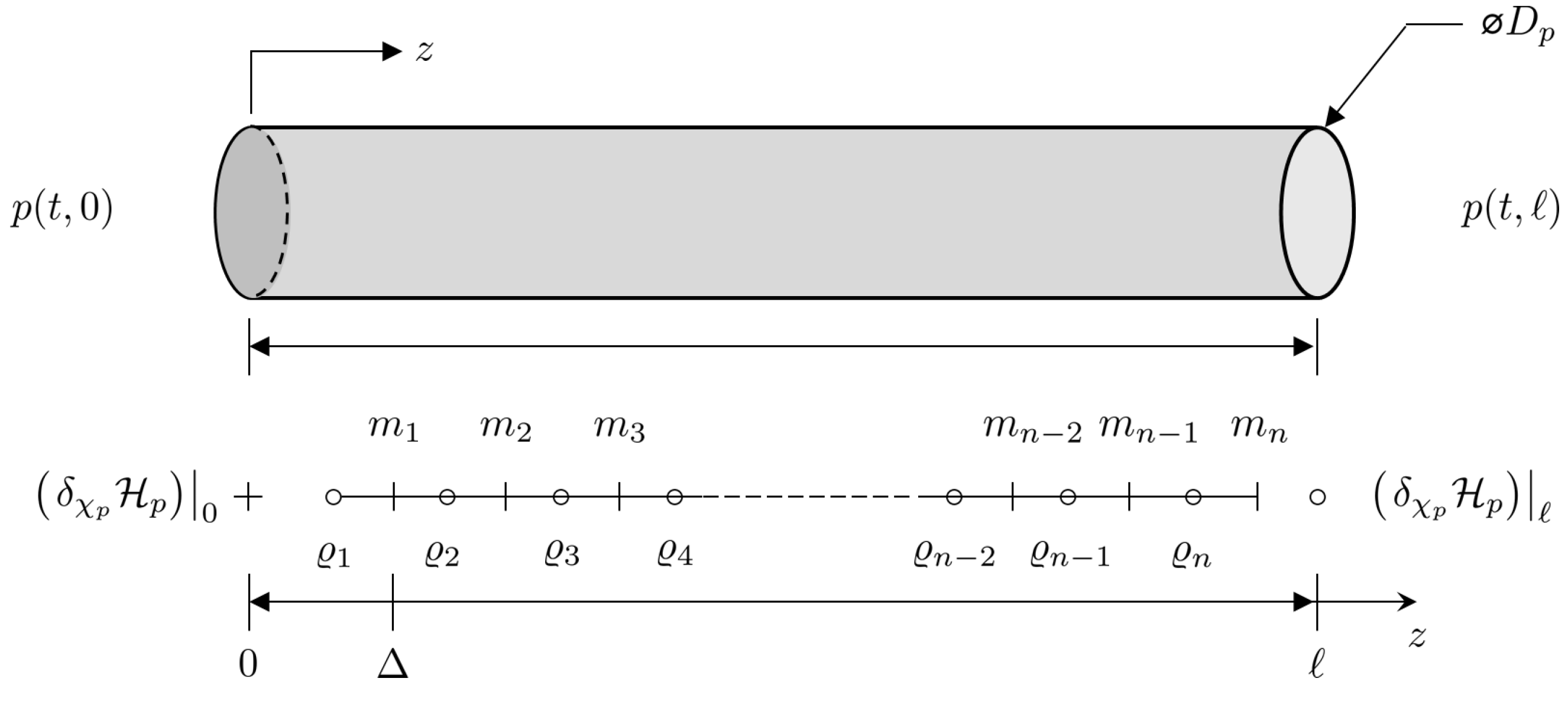
The Port–Hamiltonian model of the pipe is a partial differential equation that is continuous in space. As such, it is difficult to simulate the dynamics of a pipe section. In order to do this, it is necessary to approximate the model with a discrete model: in this case, a finite difference model that is an approximation of the original system. Within the context of Port–Hamiltonian systems, an additional requirement is the need to ensure that the discrete approximation maintains the structural properties of the original system: e.g., skew symmetry, etc.

Each system state can be replaced with a discrete approximation consisting of a total on n elements, as can be seen in Figure 10. As such, $\varrho \approx {\varrho }_d=\left[\begin{array}{cccc}{\varrho }_1,& {\varrho }_2,& \cdots ,& {\varrho }_n\end{array}\right]\in {\mathbb{R}}^{n\times 1}$, and $m\approx m_d=\left[\begin{array}{cccc}{m}_1,& m_2,& \cdots ,& m_n\end{array}\right]\in {\mathbb{R}}^{n\times 1}$. As such, state vector ${\chi }_p$ can be replaced by a discrete approximation ${\chi }_d=\left[\begin{array}{cccccc}{\varrho }_1,& \cdots ,& {\varrho }_n,& m_1,& \cdots ,& m_n\end{array}\right]\in {\mathbb{R}}^{2n\times 1}$. The $i\mathrm{th}$ element of ${\varrho }_i,m_i\in {\mathbb{R}}^{1\times 1}$ is located at $z=\left\{\Delta (i-1),\Delta (i-1/2)\right\}$, where $\Delta$ is the fixed discrete step size between points, and $i=1,2,\cdots ,n$. In addition, the efforts at the boundaries are given by ${\delta }_{{\chi }_0}{\mathcal{H}}_0$ and ${\delta }_{{\chi }_n}{\mathcal{H}}_n$. Thus, the Hamiltonian given in Equation (20) can be approximated by a discrete approximation such that ${\mathcal{H}}_p\left[{\chi }_p\right]\approx \Delta {\mathcal{H}}_d\left[{\chi }_d\right]$ so that the discrete system effort is now ${\delta }_{{\chi }_d}\left({\mathcal{H}}_d\right)$. A finite difference approximation of the spatial derivatives at the $i\mathrm{th}$ point is

$$\begin{array}{c}\hfill {\left.{\displaystyle \frac{\partial }{\partial z}}\varrho (t,z)\right|}_i\approx {\displaystyle \frac{1}{\Delta }}(\varrho (t,z_{i+0.5})-\varrho (t,z_{i-0.5}))\mathrm{and}{\left.{\displaystyle \frac{\partial }{\partial z}}m(t,z)\right|}_i\approx {\displaystyle \frac{1}{\Delta }}(m(t,z_{i+1})-m(t,z_i)).\end{array}$$

(39)

The central difference approximation at the $i\mathrm{th}$ point is

$$\begin{array}{c}\hfill {\partial }_t\left[\begin{array}{c}{\varrho }_i\\ m_i\end{array}\right]={\displaystyle \frac{1}{\Delta }}\left(\left[\begin{array}{c}{\delta }_m\mathcal{H}\left[{\chi }_i\right]\\ {\delta }_{\varrho }\mathcal{H}\left[{\chi }_{i+1}\right]\end{array}\right]-\left[\begin{array}{c}{\delta }_m\mathcal{H}\left[{\chi }_{i-1}\right]\\ {\delta }_{\varrho }\mathcal{H}\left[{\chi }_i\right]\end{array}\right]\right).\end{array}$$

(40)

In matrix form, this is

$$\begin{array}{c}\hfill {\partial }_t{\varrho }_d={\displaystyle \frac{1}{\Delta }}\left[\begin{array}{cccc}-1& & & \\ 1& -1& & \\ & \ddots & \ddots & \\ & & 1& -1\end{array}\right]{\delta }_m\mathcal{H}\left[{\chi }_d\right]+{\displaystyle \frac{1}{\Delta }}\left[\begin{array}{c}1\\ 0\\ ⋮\\ 0\end{array}\right]{\delta }_m\mathcal{H}\left[{\chi }_d\right]\end{array}$$

(41)

and

$$\begin{array}{c}\hfill {\partial }_t{m}_d={\displaystyle \frac{1}{\Delta }}\left[\begin{array}{cccc}1& -1& & \\ & \ddots & \ddots & \\ & & 1& -1\\ & & & 1\end{array}\right]{\delta }_{\varrho }\mathcal{H}\left[{\chi }_d\right]+{\displaystyle \frac{1}{\Delta }}\left[\begin{array}{c}0\\ ⋮\\ 0\\ -1\end{array}\right]{\delta }_{\varrho }\mathcal{H}\left[{\chi }_0\right],\end{array}$$

(42)

which can be re-written as

$$\begin{array}{c}\hfill {\partial }_t{\varrho }_d=D{\delta }_m\mathcal{H}\left[{\chi }_d\right]+{\mathcal{G}}_{\varrho }{\delta }_m\mathcal{H}\left[{\chi }_0\right]\mathrm{and}{\partial }_t{m}_d=-D^{\top }{\delta }_{\varrho }\mathcal{H}\left[{\chi }_d\right]+{\mathcal{G}}_m{\delta }_{\varrho }\mathcal{H}\left[{\chi }_n\right],\end{array}$$

(43)

where

$$\begin{array}{c}\hfill D={\displaystyle \frac{1}{\Delta }}\left[\begin{array}{cccc}-1& & & \\ 1& -1& & \\ & \ddots & \ddots & \\ & & 1& -1\end{array}\right],{\mathcal{G}}_{\varrho }={\displaystyle \frac{1}{\Delta }}\left[\begin{array}{c}1\\ 0\\ ⋮\\ 0\end{array}\right]\mathrm{and}{\mathcal{G}}_m={\displaystyle \frac{1}{\Delta }}\left[\begin{array}{c}0\\ ⋮\\ 0\\ -1\end{array}\right].\end{array}$$

The skew-symmetric operator is clear from Equation (43).

$$\begin{array}{ccc}\hfill \left[\begin{array}{c}{\partial }_t{\varrho }_d\\ {\partial }_t{m}_d\end{array}\right]& =& \left[\begin{array}{cc}& D\\ -D^{\top }\end{array}\right]\left[\begin{array}{c}{\delta }_{\varrho }\mathcal{H}\left[{\chi }_d\right]\\ {\delta }_m\mathcal{H}\left[{\chi }_d\right]\end{array}\right]+\left[\begin{array}{cc}& {\mathcal{G}}_m\\ {\mathcal{G}}_{\varrho }\end{array}\right]\left[\begin{array}{c}{\delta }_{\varrho }\mathcal{H}\left[{\chi }_0\right]\\ {\delta }_m\mathcal{H}\left[{\chi }_n\right]\end{array}\right].\hfill \end{array}$$

(44)

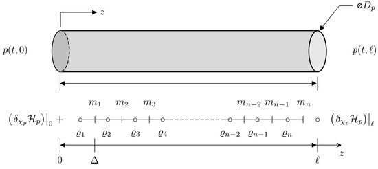
Figure 10. Staggered grid discretization of the one-dimensional Port–Hamiltonian pipe dynamic model.

8. Results and Discussion

The pipe and solenoid valve model parameters used in this work are given in Table 1 and Table 2, respectively. The Lung circuit model parameters are given in Table 3.

Table 1. Pipe model parameter values.

Parameter	Description	Value	Units
$A_p$	Pipe cross-sectional area	$3.8013\times {10}^{-4}$	m2
$D_p$	Pipe diameter	$2.2\times {10}^{-3}$	m
ℓ	Pipe length	$1.5\times {10}^{-1}$	m

Table 2. Solenoid model parameter values [28].

Parameter	Description	Value	Units
$A_e$	Effective cross-sectional area	$8\times {10}^{-5}$	m2
$A_{s_1}$	Spool surface area	$2.657\times {10}^{-3}$	m2
$A_{s_2}$	Spool surface area	$3.525\times {10}^{-3}$	m2
$A_{s_3}$	Spool surface area	$5.586\times {10}^{-3}$	m2
$A_{s_4}$	Spool surface area	$5.586\times {10}^{-3}$	m2
$b_s$	Viscous damping factor	$2\times {10}^{-1}$	Ns·m−1
g	Acceleration due to gravity	$9.81$	m·s−2
$k_s$	Spring stiffness	$1\times {10}^{-4}$	N·m−1
$l_c$	Length of the part of the magnetic circuit inside the core	$1.15\times {10}^{-2}$	m
$m_s$	Mass of the spool	$2.7\times {10}^{-1}$	kg
N	Number of turns in the coil	1250	turns
$q_{s_{\mathrm{tot}}}$	Total air gap	$3.3\times {10}^{-4}$	m
$q_{s_0}$	Pre-tension in the spring	$1.1\times {10}^{-3}$	m
$R_s$	Resistance of the coil	13	$\Omega$
${\mu }_0$	Permeability of air	$4\pi \times {10}^{-7}$	N·A−2
${\mu }_c$	Permeability of the magnetic core	$4.8\pi \times {10}^{-5}$	N·A−2

Table 3. Lung circuit model parameter values [26].

Parameter	Description	Value	Units
$R_{\mathrm{ML}}$	Resistance from the mouth to larynx	$1.021$	cmH2O·s·L−1
$R_{\mathrm{LT}}$	Resistance from the larynx to trachea	$3.369\times {10}^{-1}$	cmH2O·s·L−1
$R_{\mathrm{TB}}$	Resistance from the trachea to bronchi	$3.063\times {10}^{-1}$	cmH2O·s·L−1
$R_{\mathrm{BA}}$	Resistance from the bronchi to alveoli	$8.17\times {10}^{-2}$	cmH2O·s·L−1
$C_l$	Compliance of the larynx	$1.27\times {10}^{-3}$	L/cmH2O
$C_{\mathrm{T}}$	Compliance of the trachea	$2.38\times {10}^{-3}$	L/cmH2O
$C_{\mathrm{B}}$	Compliance of the bronchi	$1.31\times {10}^{-2}$	L/cmH2O
$C_{\mathrm{A}}$	Compliance of the alveoli	$2\times {10}^{-1}$	L/cmH2O
$C_{\mathrm{CW}}$	Compliance of the chest wall	$2.445\times {10}^{-1}$	L/cmH2O

8.1. Model Validation

The model was validated using parameters obtained from the literature. The simulation results provided in the results and discussion section were found to be comparable to those in the existing literature.

8.2. Simulation Environment

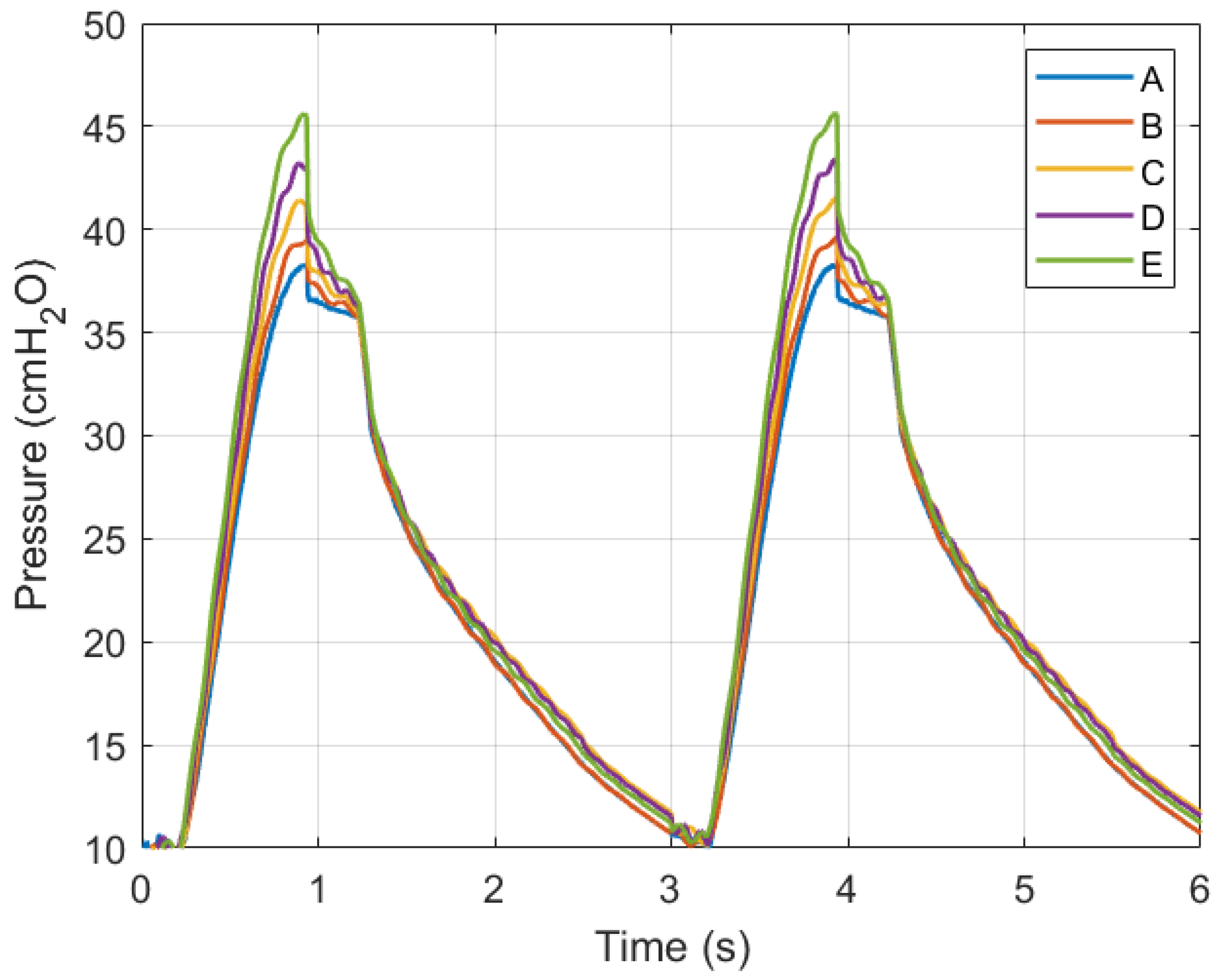
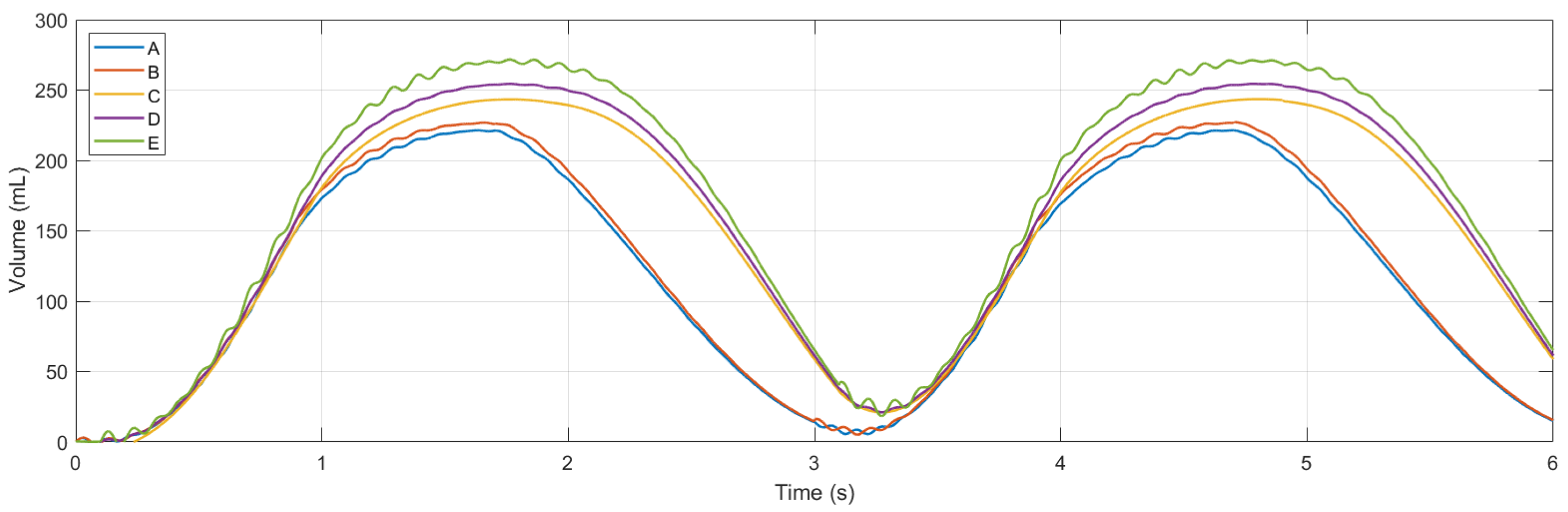
Simulations were conducted using MATLAB Version: 9.13.0.2193358 (R2022b) Update 5 on an Intel Core i5 CPU with four cores and 8 GB of RAM. Figure 11 and Figure 12 show ventilation curves for a lung under two conditions: a partially damaged lung with a compliance and resistance of 20 mL/cmH₂O and 20 cmH₂O-s/L, respectively, and a lung with complete damage, which is represented by a lung compliance and resistance of 10 mL/cmH₂O and 50 cmH₂O-s/L, respectively. The ventilation curves maintain the same sinusoidal behaviour. For the damaged lung case study, minimum ventilation values of flow over time and air volume are achieved. In the damaged lung, the compliance and resistance of the lung increase the pressure.

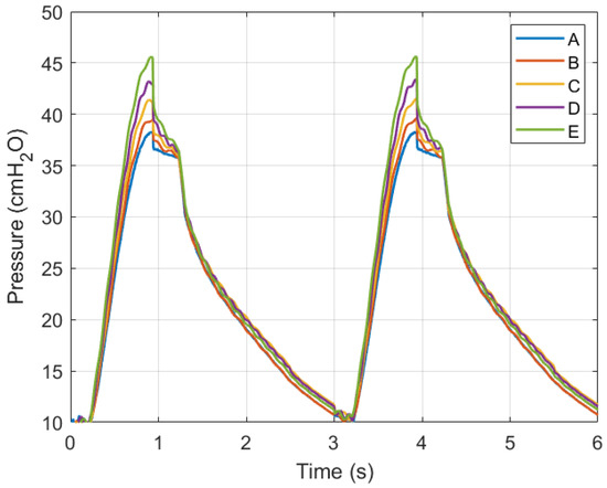
Figure 11. Graph of air pressure versus time.

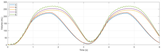
Figure 12. Graph of volume flow versus time.

9. Conclusions and Recommendations

In this research work, we formulate a detailed mechanical ventilator in the Port–Hamiltonian framework. This is followed by a Port–Hamiltonian model of the respiratory system, and thereafter, these two systems are integrated. The conducted work demonstrates that the Port–Hamiltonian approach is a valid method for the modelling of an integrated mechanical ventilator–human respiratory system. The Port–Hamiltonian framework is modular in nature. Furthermore, the complete model structure is based on the underlying graph of the mechanical ventilator and human respiratory system. Future research directions include:

• Developing a software framework for the automatic generation of the Port–Hamiltonian dynamics for various mechanical ventilator and human respiratory system configurations as well as their associated integrated models [19];
• Development of various reduced-order models;
• Development of an integrated framework for the modelling of mechanical ventilator/human respiratory systems to enable control and system optimization [19,20];
• Taking advantage of the modular and graph theoretic nature of the Port–Hamiltonian approach to incorporate machine learning and artificial intelligence [19];
• Investigation of the most appropriate structure-preserving discretizations and model-order reductions for various data-driven applications and control system designs.

References

- Rubio, J.; Rojas, C.; Sanchez, M.; Gómez-Alzate, D.; Córdova, M.; Montoya, V.; Castaneda, B.; Chang, J.; Pérez-Buitrago, S. COVOX: Providing oxygen during the COVID-19 health emergency. HardwareX 2023, 13, e00383. [Google Scholar] [CrossRef]
- Hickling, K.G. The Pressure–Volume Curve Is Greatly Modified by Recruitment. Am. J. Respir. Crit. Care Med. 1998, 158, 194–202. [Google Scholar] [CrossRef]
- Bates, J.H.T. Lung Mechanics: An Inverse Modeling Approach; Cambridge University Press: Cambridge, UK, 2009. [Google Scholar]
- Maury, B. The Respiratory System in Equations, 1st ed.; MS&A—Modeling, Simulation and Applications; Springer: Milan, Italy, 2013. [Google Scholar] [CrossRef]
- Burrowes, K.S.; Hunter, P.J.; Tawhai, M.H. Anatomically based finite element models of the human pulmonary arterial and venous trees including supernumerary vessels. J. Appl. Physiol. 2005, 99, 731–738. [Google Scholar] [CrossRef]
- Tawhai, M.H.; Bates, J.H.T. Multi-scale lung modeling. J. Appl. Physiol. 2011, 110, 1466–1472. [Google Scholar] [CrossRef]
- Berger, L.; Bordas, R.; Burrowes, K.; Brightling, C.; Hartley, R.; Kay, D. Understanding the Interdependence Between Parenchymal Deformation and Ventilation In Obstructive Lung Disease. In B30. Dynamics of Airway Narrowing in Asthma: Still Misunderstood? American Thoracic Society: New York, NY, USA, 2014; Volume 189, p. A2677. [Google Scholar]
- Roth, C.J.; Yoshihara, L.; Ismail, M.; Wall, W.A. Computational modelling of the respiratory system: Discussion of coupled modelling approaches and two recent extensions. Comput. Methods Appl. Mech. Eng. 2017, 314, 473–493. [Google Scholar] [CrossRef]
- Tran, A.S.; Thinh Ngo, H.Q.; Dong, V.K.; Vo, A.H. Design, Control, Modeling, and Simulation of Mechanical Ventilator for Respiratory Support. Math. Probl. Eng. 2021, 2021, 2499804. [Google Scholar] [CrossRef]
- El-Hadj, A.; Kezrane, M.; Ahmad, H.; Ameur, H.; Bin Abd Rahim, S.Z.; Younsi, A.; Abu-Zinadah, H. Design and simulation of mechanical ventilators. Chaos Solitons Fractals 2021, 150, 111169. [Google Scholar] [CrossRef]
- Tharion, J.; Kapil, S.; Muthu, N.; Tharion, J.; Subramani, K. Rapid Manufacturable Ventilator for Respiratory Emergencies of COVID-19 Disease. Trans. Indian Natl. Acad. Eng. 2020, 5, 373–378. [Google Scholar] [CrossRef]
- Pivik, W.J.; Clayton, G.M.; Jones, G.F.; Nataraj, C. Dynamic Modeling of a Low-cost Mechanical Ventilator. IFAC-PapersOnLine 2022, 55, 81–85. [Google Scholar] [CrossRef]
- Al-Naggar, N. Modelling and Simulation of Pressure Controlled Mechanical Ventilation System. J. Biomed. Sci. Eng. 2015, 8, 707–716. [Google Scholar] [CrossRef]
- Shi, Y.; Ren, S.; Cai, M.; Xu, W. Modelling and Simulation of Volume Controlled Mechanical Ventilation System. Math. Probl. Eng. 2014, 2014, 271053. [Google Scholar] [CrossRef]
- Al-Naggar, N.Q.; Al-Hetari, H.Y.; Al-Akwaa, F.M. Simulation of Mathematical Model for Lung and Mechanical Ventilation. J. Sci. Technol. 2016, 21, 1–9. [Google Scholar] [CrossRef]
- Giri, J.; Kshirsagar, N.; Wanjari, A. Design and simulation of AI-based low-cost mechanical ventilator: An approach. Mater. Today Proc. 2021, 47, 5886–5891. [Google Scholar] [CrossRef]
- Hannon, D.M.; Mistry, S.; Das, A.; Saffaran, S.; Laffey, J.G.; Brook, B.S.; Hardman, J.G.; Bates, D.G. Modeling Mechanical Ventilation In Silico—Potential and Pitfalls. Semin. Respir. Crit. Care Med. 2022, 43, 335–345. [Google Scholar] [CrossRef]
- Mehedi, I.M.; Shah, H.S.; Al-Saggaf, U.M.; Mansouri, R.; Bettayeb, M. Fuzzy PID control for respiratory systems. J. Healthc. Eng. 2021, 2021, 1926711. [Google Scholar] [CrossRef]
- Mehrmann, V.; Unger, B. Control of port-Hamiltonian differential-algebraic systems and applications. Acta Numer. 2023, 32, 395–515. [Google Scholar] [CrossRef]
- van der Schaft, A. Port-Hamiltonian Modeling for Control. Annu. Rev. Control Robot. Auton. Syst. 2020, 3, 393–416. [Google Scholar] [CrossRef]
- Villegas, J.A. A Port-Hamiltonian Approach to Distributed Parameter Systems. Ph.D. Thesis, Department of Applied Mathematics, Faculty EWI, Universiteit Twente, Enschede, The Netherlands, 2007. [Google Scholar]
- Le Gorrec, Y.; Zwart, H.; Maschke, B. Dirac structures and Boundary Control Systems associated with Skew-Symmetric Differential Operators. SIAM J. Control Optim. 2005, 44, 1864–1892. [Google Scholar] [CrossRef]
- van der Schaft, A.J.; Maschke, B.M. Hamiltonian formulation of distributed-parameter systems with boundary energy flow. J. Geom. Phys. 2002, 42, 166–194. [Google Scholar] [CrossRef]
- Anderson, J. Computational Fluid Dynamics: The Basics with Applications; McGraw-Hill International Editions: Mechanical Engineering; McGraw-Hill Inc.: New York, NY, USA, 1995. [Google Scholar]
- Kamiński, Z. A simplified lumped parameter model for pneumatic tubes. Math. Comput. Model. Dyn. Syst. 2017, 23, 523–535. [Google Scholar] [CrossRef]
- Albanese, A.; Cheng, L.; Ursino, M.; Chbat, N.W. An integrated mathematical model of the human cardiopulmonary system: Model development. Am. J. Physiol.-Heart Circ. Physiol. 2016, 310, H899–H921. [Google Scholar] [CrossRef] [PubMed]
- Bondy, J.A.; Murty, U.S.R. Graph Theory with Applications; The Macmillan Press Ltd.: London, UK, 1976. [Google Scholar]
- Taghizadeh, M.; Ghaffari, A.; Najafi, F. Modeling and identification of a solenoid valve for PWM control applications. Comptes Rendus Mécanique 2009, 337, 131–140. [Google Scholar] [CrossRef]
Disclaimer/Publisher’s Note: The statements, opinions and data contained in all publications are solely those of the individual author(s) and contributor(s) and not of MDPI and/or the editor(s). MDPI and/or the editor(s) disclaim responsibility for any injury to people or property resulting from any ideas, methods, instructions or products referred to in the content. |
© 2024 by the authors. Licensee MDPI, Basel, Switzerland. This article is an open access article distributed under the terms and conditions of the Creative Commons Attribution (CC BY) license (https://creativecommons.org/licenses/by/4.0/).