The Effect of Proportional, Proportional-Integral, and Proportional-Integral-Derivative Controllers on Improving the Performance of Torsional Vibrations on a Dynamical System

Abstract

The primary goal of this research is to lessen the high vibration that the model causes by using an appropriate vibration control. Thus, we begin by implementing various controller types to investigate their impact on the system’s reaction and evaluate each control’s outcomes. The controller types are presented as proportional (P), proportional-integral (PI), and proportional-integral-derivative (PID) controllers. We employed PID control to regulate the torsional vibration behavior on a dynamical system. The PID controller aims to increase system stability after seeing the impact of P and PI control. This kind of control ensures that there are no unstable components in the system. By using the multiple time scale perturbation (MTSP) technique, a first-order approximate solution has been obtained. Using the frequency response function approach, the stability and steady-state response of the system at the primary resonance scenario (${\mathsf{\Omega }}_1\cong {\omega }_1,{\mathsf{\Omega }}_2\cong {\omega }_2$) are considered as the worst resonance and addressed. Additionally examined are the nonlinear dynamical system’s chaotic response and the numerical solution for various parameter values. The MATLAB programs are utilized to attain simulation outcomes.

1. Introduction

Torsional vibration occurs in some form in all rotating machinery. Even when the vibration is nearing destructive amplitude, there are situations in which it cannot be identified without specialized monitoring equipment. After the shaft bending stiffness and diametral moment of inertia have been replaced by the twisting stiffness and polar moment of inertia, respectively, many elements of torsional vibration are equivalent to shaft vibration. When something mediates the connection between the vibration and the ground, or when gear teeth or coupling jaws are empty, torsional vibration can be detected by the noise level and vibration (perceptible to touch). Torsional vibration can interact with the ground through gear sets used to change the speed of power transmission systems; in reciprocating machines, the path to the ground is provided by sliding crank mechanisms found in engines and compressors. Typically, torsional vibration manifests as a complicated vibration signal with numerous frequency components. Some systems experience brief torsional vibrations due to shock from sudden starts and the unloading of gear teeth; synchronous electric motor systems may also experience torsional resonance at startup.

Conventional PID controllers have been widely adopted in numerous industrial applications due to their simple design, affordable price, simplicity of maintenance, and there being ready-made modules [1,2,3]. Ref. [4] offers the implementation of nonlinear state-dependent (SDP-PID+) control employing the SDP transfer function model, a type of nonlinear description of dynamical structures. Fine-tuning traditional PID control is problematic owing to the specific properties of numerous procedures, including binary sample time delays, longer durations, higher-order TF models, and nonlinearities [5,6,7]. Sayed et al. [8] developed a nonlinear resilient SDP PID control approach for a discrete transfer function with nonlinear properties. This research emphasized robust response processes, for which the robust PID and SDP-PID techniques were specifically designed. Dano and Julli’ere [9] studied how MFC actuators controlled oscillations in a composite structure. Kumar and Ray [10] examined vibrations in sandwich shells with between one and three piezoelectric composites and layering damping techniques. The PD controller is designed to decrease oscillations of a hung Jeffcott rotor through two pairs of poles [11]. A PD controller can effectively relax a beam system’s steady-state amplitude vibrations [12]. Eissa et al. [13,14] suggested a PD controller and a time-delayed PD controller to reduce the vibrations of magnetic systems with cubic and quadratic nonlinear coefficients underneath parametric principal forces. Bauomy and El-Sayed employed a PD controller to control the behavior of the MFC laminated shell structure. The purpose of employing the PD controller is to improve system stability by increasing control, as it can forecast future errors in the framework response [15]. More than 90% of industries still utilize PID controllers due to their simplicity, functionality, and ease of usage [16]. PID controller gains are acquired by matching the frequency response of the closed-loop control system [17]. Recently, a systematic approach was used to select PID parameters for nonlinear uncertain structures [18]. PID controllers offer advantages over passive approaches for controlling semi-active suspension systems [19,20,21]. Ref. [22] investigates the control of a quarter-car semi-active suspension system utilizing a PID controller. The typical PID controller is constructed using the Ziegler–Nichols approach and is used to regulate the suspension system. The torsional vibrations of a one-degree-of-freedom nonlinear dynamical structure are regulated with active control [23]. Wenzhi and Zhiyong [24] suggested an active control to decrease torsional vibration in a big turbogenerator with a rotor shaft. Whole-state feedback control using a linear quadratic regulator (LQR) effectively reduces torsional vibration energy and response in the turbogenerator shaft system. El-Sayed and Bauomy [25] they succeeded in reducing the torsional vibration of a nonlinear dynamical system using passive and active control methods. The research study [26] proposes an adaptive PI event-triggered control approach for MIMO nonlinear systems with unpredictable input delay. An adaptive proportional/proportional-integral (P/PI) control strategy is proposed for a solar-driven volumetric methane/steam reforming reactor (SVMSR) with passive thermal management. The strategy aims to stabilize product components and reduce fluctuations in the hydrogen production rate under fluctuating radiation conditions [27]. Previous research, such as studies [28,29,30], has demonstrated the successful application of the multiple-scale perturbation technique to derive approximate solutions for various vibrating systems. These studies often utilize MATLAB programs to analyze and solve vibration problems.

A cantilever beam model was explored and derived to load an intermediate lumped mass under harmonic excitation. The vibration suppression can be succeeded by using IRC+ NSC controller. To determine the unstable and stable zones for each frequency response curve, numerical stability research was carried out [31].This research investigates the use of a nonlinear spring pendulum for the vibration control of ship roll motion. Three second-order nonlinear differential equations—one for the rotation angle, one for the relative elongation of the absorber spring, and one for the elongation of the absorber spring—make up the mathematical model that depicts the ship roll motion with the absorber. The authors use a series solution in which they account for terms up to the fourth order in trigonometric functions of the rotational angle. According to the authors, the nonlinear spring-pendulum system’s two modes may be made to respond to multi-parametric excitation forces in a way that reduces their maximum values by 8.8% and 0.02% [32]. The PPF control of the nonlinear GMA framework has been described in [33]. The basic resonance and framework amplitude stability can be successfully constrained by tuning the PPF limitations. A few experiments have been carried out to verify the accuracy of the findings. The investigation illustrated the growth of the framework and contrasted its usefulness to earlier research. The 3D plot improves and illustrates the work’s correctness. Ref. [34] suggests using NIPPF controllers to manage the nonlinear vibration of a spinning shaft’s primary resonance vibration. Among these is a comparison between the controllers for the FRCs under study, NIPPF, and ANIPPF. A two-degree-of-freedom system, counting quadratic and cubic nonlinearities among the parametric and external forces, demonstrate the calculated system. Multiple scales are joined in a connected manner to analyze the stability of the measured structure and obtain approximations of solutions. From the mathematical solution, every resonance is retrieved. The Runge–Kutta fourth-order process is used to gauge the system’s performance. Within the numerical results, the examined structure’s scheduled frequency response curves are examined for influences including significant coefficients [35]. A low-speed and high-torque permanent magnet synchronous motor powers the semi-direct drive-cutting gearbox system of a shearer, which uses nonlinear integral positive position feedback (NIPPF) and adaptive nonlinear integral positive position feedback (ANIPPF) controllers. Using the averaging technique to solve the nonlinear differential equations and modeling the system with controllers yields an analytic solution in the case of primary and 1:1 internal resonance. The MATLAB program was used to compare the numerical and analytical solutions for time history and FRCs in order to verify their comparability [36].

In this work, we utilized PID control to suppress the torsional vibration after studying the model on a website [37]. A two-degree-of-freedom system under multiple excitations results from this. To provide an estimated solution up to the first-order approximations, MSPT is employed throughout. Using frequency response functions, the stability of the system is examined in the vicinity of the principal resonance case. A few suggestions on the system’s various parameters are given. Numerical examples are provided to show how active controllers affect the behavior of the system. A comparison is shown between PID control and additional controllers.

2. Mathematical Modeling

2.1. System Dynamics without Control

This section is presented to illustrate the investigation of the torsional vibration dynamical system. The dynamical model in this work consists of two coupled parts, as shown in Figure 1. ${\theta }_1$ and ${\theta }_2$ represent the angular positions (generalized coordinates) within the system. In this nonlinear dynamical system, the following hold:

• $I_1$ and $I_2$ represent the polar mass moments of inertia.
• $k_1$ is the linear spring stiffness of the first part.
• $k_2$ represents the spring stiffness of the second part, which comprises the following:

  ◦

  $k_{21}$: a linear component.

  ◦

  $k_{22}$: nonlinear quadratic and cubic components.

• $F_1^{•}$ and $F_2^{•}$ denote the generalized excitation forces.

Therefore, the equations of the motions of the free body system found in Figure 1 can be constructed in the same manner as those in [25,37]:

$$I_1{\ddot{\theta }}_1+k_1{\theta }_1+c_1{\dot{\theta }}_1+k_{21}\left({\theta }_1-{\theta }_2\right)+k_{22}{\left({\theta }_1-{\theta }_2\right)}^2+k_{23}{\left({\theta }_1-{\theta }_2\right)}^3=F_1^{•},$$

(1)

$$I_2{\ddot{\theta }}_2+k_{21}\left({\theta }_2-{\theta }_1\right)-k_{22}{\left({\theta }_1-{\theta }_2\right)}^2-k_{23}{\left({\theta }_1-{\theta }_2\right)}^3=F_2^{•},$$

(2)

$${\ddot{\theta }}_1+{\displaystyle \frac{k_1}{I_1}}{\theta }_1+{\displaystyle \frac{c_1}{I_1}}{\dot{\theta }}_1+{\displaystyle \frac{k_{21}}{I_1}}\left({\theta }_1-{\theta }_2\right)+{\displaystyle \frac{k_{22}}{I_1}}{\left({\theta }_1-{\theta }_2\right)}^2+{\displaystyle \frac{k_{23}}{I_1}}{\left({\theta }_1-{\theta }_2\right)}^3={\displaystyle \frac{F_1^{•}}{I_1}},$$

(3)

$${\ddot{\theta }}_1+\left({\displaystyle \frac{k_1+k_{21}}{I_1}}\right){\theta }_1+{\displaystyle \frac{c_1}{I_1}}{\dot{\theta }}_1-{\displaystyle \frac{k_{21}}{I_1}}{\theta }_2+{\displaystyle \frac{k_{22}}{I_1}}{\left({\theta }_1-{\theta }_2\right)}^2+{\displaystyle \frac{k_{23}}{I_1}}{\left({\theta }_1-{\theta }_2\right)}^3={\displaystyle \frac{F_1^{•}}{I_1}},$$

(4)

$${\ddot{\theta }}_2+{\displaystyle \frac{k_{21}}{I_2}}\left({\theta }_2-{\theta }_1\right)-{\displaystyle \frac{k_{22}}{I_2}}{\left({\theta }_1-{\theta }_2\right)}^2-{\displaystyle \frac{k_{23}}{I_2}}{\left({\theta }_1-{\theta }_2\right)}^3={\displaystyle \frac{F_2^{•}}{I_2}},$$

(5)

$${\displaystyle \frac{{\ddot{\theta }}_1}{{\theta }_0}}+\left({\displaystyle \frac{k_1+k_{21}}{I_1}}\right){\displaystyle \frac{{\theta }_1}{{\theta }_0}}+{\displaystyle \frac{c_1}{I_1}}{\displaystyle \frac{{\dot{\theta }}_1}{{\theta }_0}}-{\displaystyle \frac{k_{21}}{I_1}}{\displaystyle \frac{{\theta }_2}{{\theta }_0}}+{\displaystyle \frac{k_{22}{\theta }_0}{I_1}}{\displaystyle \frac{{\left({\theta }_1-{\theta }_2\right)}^2}{{\theta }_0^2}}+{\displaystyle \frac{k_{23}{\theta }_0^2}{I_1}}{\displaystyle \frac{{\left({\theta }_1-{\theta }_2\right)}^3}{{\theta }_0^3}}={\displaystyle \frac{F_1^{•}}{I_1}},$$

(6)

$${\displaystyle \frac{{\ddot{\theta }}_2}{{\theta }_0}}+{\displaystyle \frac{k_{21}}{I_2}}{\displaystyle \frac{\left({\theta }_2-{\theta }_1\right)}{{\theta }_0}}-{\displaystyle \frac{k_{22}{\theta }_0}{I_2}}{\displaystyle \frac{{\left({\theta }_1-{\theta }_2\right)}^2}{{\theta }_0^2}}-{\displaystyle \frac{k_{23}{\theta }_0^2}{I_2}}{\displaystyle \frac{{\left({\theta }_1-{\theta }_2\right)}^3}{{\theta }_0^3}}={\displaystyle \frac{F_2^{•}}{I_2}}.$$

(7)

We will now introduce the dimensionless forms of the parameters used in this analysis.

$${\phi }_j={\displaystyle \frac{{\theta }_j}{{\theta }_0}}\left(j=1,2\right),{\omega }_1^2={\displaystyle \frac{k_1+k_{21}}{I_1}},\zeta ={\displaystyle \frac{c_1}{I_1}},\beta ={\displaystyle \frac{k_{21}}{I_1}},{\alpha }_1={\displaystyle \frac{k_{22}{\theta }_0}{I_1}},{\alpha }_2={\displaystyle \frac{k_{23}{\theta }_0^2}{I_1}}{\omega }_2^2={\displaystyle \frac{k_{21}}{I_2}},{\alpha }_3={\displaystyle \frac{k_{22}{\theta }_0}{I_2}},$$

$${\alpha }_4={\displaystyle \frac{k_{23}{\theta }_0^2}{I_2}},\hspace{1em}{f}_j\sin ({\mathsf{\Omega }}_{j}t)={\displaystyle \frac{F_j^{•}}{I_j}}.$$

Based on the above parameters, we can obtain the following equations of motion in their dimensionless forms:

$${\ddot{\phi }}_1+{\omega }_1^2{\phi }_1+\zeta {\dot{\phi }}_1-\beta {\phi }_2+{\alpha }_1{\left({\phi }_1-{\phi }_2\right)}^2+{\alpha }_2{\left({\phi }_1-{\phi }_2\right)}^3=f_1\sin ({\mathsf{\Omega }}_{1}t),$$

(8)

$${\ddot{\phi }}_2+{\omega }_2^2\left({\phi }_2-{\phi }_1\right)-{\alpha }_3{\left({\phi }_1-{\phi }_2\right)}^2-{\alpha }_4{\left({\phi }_1-{\phi }_2\right)}^3=f_2\sin ({\mathsf{\Omega }}_{2}t).$$

(9)

2.2. System Dynamics with PID Control

The goal of the present section is to propose PID controllers to reduce harmful torsional vibration on the dynamical system in this work at one of the worst resonance cases, as depicted in Figure 2. Furthermore, the control in our work is represented as two net control forces $F_{C1}$ and $F_{C2}$ that are generated to suppress the torsional oscillations in two directions.

Here, $K_p$, $K_i$, and $K_d$ denote the proportional feedback control gain, integral feedback control gain, and derivative feedback control gain, respectively. Also, $e_1\left(t\right)$ and $e_2\left(t\right)$ denote the error value with zero steady-state step error.

The equations of motion utilizing the PID controllers coupled to the nonlinear dynamical system as depicted in Figure 2 can be expressed as follows:

$${\ddot{\phi }}_1+{\omega }_1^2{\phi }_1+\epsilon \zeta {\dot{\phi }}_1-\epsilon \beta {\phi }_2+\epsilon {\alpha }_1{\left({\phi }_1-{\phi }_2\right)}^2+\epsilon {\alpha }_2{\left({\phi }_1-{\phi }_2\right)}^3=\epsilon f_1\sin ({\mathsf{\Omega }}_{1}t)+\epsilon F_{C1},$$

(10)

$${\ddot{\phi }}_2+{\omega }_2^2\left({\phi }_2-{\phi }_1\right)-\epsilon {\alpha }_3{\left({\phi }_1-{\phi }_2\right)}^2-\epsilon {\alpha }_4{\left({\phi }_1-{\phi }_2\right)}^3=\epsilon f_2\sin ({\mathsf{\Omega }}_{2}t)+\epsilon F_{C2},$$

(11)

$$F_{C1}=-K_p{\phi }_1-K_i{\displaystyle \underset{o}{\overset{t}{\int }}{\phi }_1\left(\tau \right)d\tau }-K_d{\dot{\phi }}_1,$$

(12a)

$$F_{C2}=-K_p{\phi }_2-K_i{\displaystyle \underset{o}{\overset{t}{\int }}{\phi }_2\left(\tau \right)d\tau }-K_d{\dot{\phi }}_2,$$

(12b)

$$\begin{array}{l}{\ddot{\phi }}_1+{\omega }_1^2{\phi }_1+\epsilon \zeta {\dot{\phi }}_1-\epsilon \beta {\phi }_2+\epsilon {\alpha }_1{\left({\phi }_1-{\phi }_2\right)}^2+\epsilon {\alpha }_2{\left({\phi }_1-{\phi }_2\right)}^3=\epsilon f_1\sin ({\mathsf{\Omega }}_{1}t)\\ -\epsilon K_p{\phi }_1-\epsilon K_i{\displaystyle \underset{o}{\overset{t}{\int }}{\phi }_1\left(\tau \right)d\tau }-\epsilon K_d{\dot{\phi }}_1\end{array},$$

(13)

$$\begin{array}{l}{\ddot{\phi }}_2+{\omega }_2^2\left({\phi }_2-{\phi }_1\right)-\epsilon {\alpha }_3{\left({\phi }_1-{\phi }_2\right)}^2-\epsilon {\alpha }_4{\left({\phi }_1-{\phi }_2\right)}^3=\epsilon f_2\sin ({\mathsf{\Omega }}_{2}t)\\ -\epsilon K_p{\phi }_2-\epsilon K_i{\displaystyle \underset{o}{\overset{t}{\int }}{\phi }_2\left(\tau \right)d\tau }-\epsilon K_d{\dot{\phi }}_2\end{array}.$$

(14)

3. Analytical Investigations

3.1. Perturbation Analysis

The multiple-scales perturbation technique (MSPT) is applied within this section to obtain an approximation solution of the nonlinear dynamical system with the proposal control (i.e., PID control) given by Equations (13) and (14). Correspondingly, we were able to find a first-order approximate solution to Equations (13) and (14), proposed as follows [28,29]:

$${\phi }_n={\phi }_{n0}+\epsilon {\phi }_{n1}+O\left({\epsilon }^2\right),\hspace{1em}\hspace{1em}\left(n=1,2\right)$$

(15)

where the minor perturbation parameter $\epsilon$ is located in the range of $0<\epsilon \ll 1$. Let us define two time scales, $T_0$ and $T_1$, where $T_0=t$ represents a fast scale while $T_1=\epsilon t$ is the slow one. The derivatives of time are converted into the following:

$${\displaystyle \frac{d}{dt}}={\displaystyle \frac{d{T}_0}{dt}}{\displaystyle \frac{\partial }{\partial T_0}}+{\displaystyle \frac{d{T}_1}{dt}}{\displaystyle \frac{\partial }{\partial T_1}}+\dots =D_0+\epsilon D_1+\dots ,$$

(16)

$${\displaystyle \frac{d^2}{d{t}^2}}={\displaystyle \frac{d}{dt}}\left({\displaystyle \frac{d{T}_0}{dt}}{\displaystyle \frac{\partial }{\partial T_0}}+{\displaystyle \frac{d{T}_1}{dt}}{\displaystyle \frac{\partial }{\partial T_1}}+\dots \right)=D_0^2+2\epsilon D_0{D}_1+\dots .$$

(17)

where $D_j={\displaystyle \frac{\partial }{\partial T_j}}\hspace{1em}\left(j=0,1\right)$.

The following set of ordinary differential equations was constructed by substituting Equations (15) and (16) into Equations (13) and (14) and equating the coefficients of the same power of $\epsilon$ in both sides:

$O\left({\epsilon }^0\right)$:

$$\left(D_0^2+{\omega }_1^2\right){\phi }_{10}=0,$$

(18a)

$$\left(D_0^2+{\omega }_2^2\right){\phi }_{20}={\omega }_2^2{\phi }_{10}.$$

(18b)

$O\left({\epsilon }^1\right)$:

$$\begin{array}{l}\left(D_0^2+{\omega }_1^2\right){\phi }_{11}=-2D_0{D}_1{\phi }_{10}-\zeta D_0{\phi }_{10}+\beta {\phi }_{20}-{\alpha }_1{\left({\phi }_{10}-{\phi }_{20}\right)}^2-{\alpha }_2{\left({\phi }_{10}-{\phi }_{20}\right)}^3\\ +f_1\sin ({\mathsf{\Omega }}_{1}t)-K_p{\phi }_{10}-K_i{\displaystyle \underset{o}{\overset{t}{\int }}{\phi }_{10}\left(\tau \right)d\tau }-K_d{D}_0{\phi }_{10}\end{array},$$

(19a)

$$\begin{array}{l}\left(D_0^2+{\omega }_2^2\right){\phi }_{21}={\omega }_2^2{\phi }_{11}-2D_0{D}_1{\phi }_{20}+{\alpha }_3{\left({\phi }_{10}-{\phi }_{20}\right)}^2+{\alpha }_4{\left({\phi }_{10}-{\phi }_{20}\right)}^3+f_2\sin ({\mathsf{\Omega }}_{2}t)\\ -K_p{\phi }_{20}-K_i{\displaystyle \underset{o}{\overset{t}{\int }}{\phi }_{20}\left(\tau \right)d\tau }-K_d{D}_0{\phi }_{20}\end{array}.$$

(19b)

The zeroth order approximation is represented by the general solution of Equations (18a) and (18b), which can be expressed as follows:

$${\phi }_{10}=A_1(T_1)\exp (i{\omega }_1{T}_0)+cc.,$$

(20a)

$${\phi }_{20}=A_2(T_1)\exp (i{\omega }_2{T}_0)+\mathsf{\Gamma }{A}_1(T_1)\exp (i{\omega }_1{T}_0)+cc.$$

(20b)

where $cc$ denotes the complex conjugate of the preceding components, $A_m$ is the complex function in $T_1$, and $\mathsf{\Gamma }=\left({\displaystyle \frac{{\omega }_2^2}{{\omega }_2^2-{\omega }_1^2}}\right)$.

Substituting Equation (20) into Equation (19a), we have

$$\begin{array}{l}\left(D_0^2+{\omega }_1^2\right){\phi }_{11}=\left[\begin{array}{l}-2i{\omega }_1{D}_1{A}_1-i{\omega }_1\zeta A_1+\mathsf{\Gamma }\beta A_1-{\alpha }_2\left(\begin{array}{l}6\left(1-\mathsf{\Gamma }\right)A_1{A}_2{\overline{A}}_2\\ +3{\left(1-\mathsf{\Gamma }\right)}^3{A}_1^2{\overline{A}}_1\end{array}\right)\\ -\left(K_p-i{\displaystyle \frac{K_i}{{\omega }_1}}+K_{d}i{\omega }_1\right)A_1\end{array}\right]\exp (i{\omega }_1{T}_0)\\ +\left[-{\alpha }_1{\left(1-\mathsf{\Gamma }\right)}^2{A}_1^2\right]\exp (2i{\omega }_1{T}_0)+\left[-{\alpha }_2{\left(1-\mathsf{\Gamma }\right)}^3{A}_1^3\right]\exp (3i{\omega }_1{T}_0)+\left[\beta A_2\right.\\ +\left.{\alpha }_2\left(3A_2^2{\overline{A}}_2+6{\left(1-\mathsf{\Gamma }\right)}^2{A}_1{\overline{A}}_1{A}_2\right)\right]\exp (i{\omega }_2{T}_0)+\left[-{\alpha }_1{A}_1^2\right]\exp (2i{\omega }_2{T}_0)\\ +\left[{\alpha }_2{A}_2^3\right]\exp (3i{\omega }_2{T}_0)+\left[2{\alpha }_1\left(1-\mathsf{\Gamma }\right)A_1{A}_2\right]\exp (i\left({\omega }_1+{\omega }_2\right)T_0)\\ +\left[2{\alpha }_1\left(1-\mathsf{\Gamma }\right)A_1{\overline{A}}_2\right]\exp (i\left({\omega }_1-{\omega }_2\right)T_0)+\left[3{\alpha }_2{\left(1-\mathsf{\Gamma }\right)}^2{A}_1^2{A}_2\right]\exp (i\left(2{\omega }_1+{\omega }_2\right)T_0)\\ +\left[3{\alpha }_2{\left(1-\mathsf{\Gamma }\right)}^2{A}_1^2{\overline{A}}_2\right]\exp (i\left(2{\omega }_1-{\omega }_2\right)T_0)+\left[-3{\alpha }_2\left(1-\mathsf{\Gamma }\right)A_1{A}_2^2\right]\exp (i\left({\omega }_1+2{\omega }_2\right)T_0)\\ +\left[-3{\alpha }_2\left(1-\mathsf{\Gamma }\right)A_1{\overline{A}}_2^2\right]\exp (i\left({\omega }_1-2{\omega }_2\right)T_0)+\left[-{\alpha }_1\left({\left(1-\mathsf{\Gamma }\right)}^2{A}_1{\overline{A}}_1+A_2{\overline{A}}_2\right)-i{K}_i{\displaystyle \frac{A_1}{{\omega }_1}}\right]\\ +\left[{\displaystyle \frac{-i{f}_1}{2}}\right]\exp (i{\mathsf{\Omega }}_1{T}_0)+cc.,\end{array}$$

(21)

To obtain the solvability condition of Equation (21), the closeness term of the excitation frequencies (${\mathsf{\Omega }}_1$) and natural frequency (${\omega }_1$) is described via employing the dimensionless detuning parameter${\sigma }_1$, as in the following:

$${\mathsf{\Omega }}_1={\omega }_1+\epsilon {\sigma }_1.$$

(22)

By substituting Equation (22) into Equation (21) and canceling the term that leads to secular ones, we obtain the particular solution of the first approximation (${\phi }_{11}$) as the following:

$$\begin{array}{l}{\phi }_{11}=M_1\exp (2i{\omega }_1{T}_0)+M_2\exp (3i{\omega }_1{T}_0)+M_3\exp (i{\omega }_2{T}_0)+M_4\exp (2i{\omega }_2{T}_0)\\ +M_5\exp (3i{\omega }_2{T}_0)+M_6\exp (i\left({\omega }_1+{\omega }_2\right)T_0)+M_7\exp (i\left({\omega }_1-{\omega }_2\right)T_0)\\ +M_8\exp (i\left(2{\omega }_1+{\omega }_2\right)T_0)+M_9\exp (i\left(2{\omega }_1-{\omega }_2\right)T_0)+M_{10}\exp (i\left({\omega }_1+2{\omega }_2\right)T_0)\\ +M_{11}\exp (i\left({\omega }_1-2{\omega }_2\right)T_0)+M_{12}+cc.\end{array},$$

(23)

Here, $M_i\hspace{1em}\left(i=1,2,\dots ,12\right)$ is presented in Appendix A.

Substituting Equations (20) and (23) into Equation (19b), we have

$$\begin{array}{l}\left(D_0^2+{\omega }_2^2\right){\phi }_{21}=\left[-2i{\omega }_1{D}_1\mathsf{\Gamma }{A}_1+{\alpha }_4\left(3{\left(1-\mathsf{\Gamma }\right)}^3{A}_1^2{\overline{A}}_1+6\left(1-\mathsf{\Gamma }\right)A_1{A}_2{\overline{A}}_2\right)\right.\\ \left.-\left(K_p-i{\displaystyle \frac{K_i}{{\omega }_1}}+i{\omega }_1{K}_d\right)\mathsf{\Gamma }{A}_1\right]\exp (i{\omega }_1{T}_0)+\left[{\omega }_2^2{M}_1+{\alpha }_3{\left(1-\mathsf{\Gamma }\right)}^2{A}_1^2\right]\exp (2i{\omega }_1{T}_0)\\ +\left[{\omega }_2^2{M}_2+{\alpha }_4{\left(1-\mathsf{\Gamma }\right)}^3{A}_1^3\right]\exp (3i{\omega }_1{T}_0)+\left[{\omega }_2^2{M}_3-2i{\omega }_2{D}_1{A}_2\right.\\ -\left(K_p-i{\displaystyle \frac{K_i}{{\omega }_2}}+i{\omega }_2{K}_d\right)A_2\left.-{\alpha }_4\left(3A_2^2{\overline{A}}_2+6{\left(1-\mathsf{\Gamma }\right)}^2{A}_1{\overline{A}}_1{A}_2\right)\right]\exp (i{\omega }_2{T}_0)\\ +\left[{\omega }_2^2{M}_4+{\alpha }_3{A}_2^2\right]\exp (2i{\omega }_2{T}_0)+\left[{\omega }_2^2{M}_5-{\alpha }_4{A}_2^3\right]\exp (3i{\omega }_2{T}_0)\\ +\left[{\omega }_2^2{M}_6-2{\alpha }_3\left(1-\mathsf{\Gamma }\right)A_1{A}_2\right]\exp (i\left({\omega }_1+{\omega }_2\right)T_0)+\left[{\omega }_2^2{M}_7-2{\alpha }_3\left(1-\mathsf{\Gamma }\right)A_1{\overline{A}}_2\right]\\ \times \exp (i\left({\omega }_1-{\omega }_2\right)T_0)+\left[{\omega }_2^2{M}_8-3{\alpha }_4{\left(1-\mathsf{\Gamma }\right)}^2{A}_1^2{A}_2\right]\exp (i\left(2{\omega }_1+{\omega }_2\right)T_0)\\ +\left[{\omega }_2^2{M}_9-3{\alpha }_4{\left(1-\mathsf{\Gamma }\right)}^2{A}_1^2{\overline{A}}_2\right]\exp (i\left(2{\omega }_1-{\omega }_2\right)T_0)+\left[{\omega }_2^2{M}_{10}+3{\alpha }_4\left(1-\mathsf{\Gamma }\right)A_1{A}_2^2\right]\\ \times \exp (i\left({\omega }_1+2{\omega }_2\right)T_0)+\left[{\omega }_2^2{M}_{11}+3{\alpha }_4\left(1-\mathsf{\Gamma }\right)A_1{\overline{A}}_2^2\right]\exp (i\left({\omega }_1-2{\omega }_2\right)T_0)\\ +\left[{\omega }_2^2{M}_{12}+{\alpha }_3\left({\left(1-\mathsf{\Gamma }\right)}^2{A}_1{\overline{A}}_1+A_2{\overline{A}}_2\right)-K_i\left(i{\displaystyle \frac{A_2}{{\omega }_2}}+i{\displaystyle \frac{\mathsf{\Gamma }{A}_1}{{\omega }_1}}\right)\right]+\left[{\displaystyle \frac{-i{f}_2}{2}}\right]\exp (i{\mathsf{\Omega }}_2{T}_0)+cc.\end{array}$$

(24)

To obtain the second solvability condition of Equation (24), the closeness term of excitation frequencies (${\mathsf{\Omega }}_2$) and natural frequency (${\omega }_2$) is described via employing the dimensionless detuning parameter ${\sigma }_2$ as the following:

$${\mathsf{\Omega }}_2={\omega }_2+\epsilon {\sigma }_2.$$

(25)

By substituting Equation (25) into Equation (24) and canceling the term which leads to the secular ones, we obtain the particular solution of the first approximation (${\phi }_{21}$) as the following:

$$\begin{array}{l}{\phi }_{21}=N_1\exp (i{\omega }_1{T}_0)+N_2\exp (2i{\omega }_1{T}_0)+N_3\exp (3i{\omega }_1{T}_0)+N_4\exp (2i{\omega }_2{T}_0)\\ +N_5\exp (3i{\omega }_2{T}_0)+N_6\exp (i\left({\omega }_1+{\omega }_2\right)T_0)+N_7\exp (i\left({\omega }_1-{\omega }_2\right)T_0)\\ +N_8\exp (i\left(2{\omega }_1+{\omega }_2\right)T_0)+N_9\exp (i\left(2{\omega }_1-{\omega }_2\right)T_0)+N_{10}\exp (i\left({\omega }_1+2{\omega }_2\right)T_0)\\ +N_{11}\exp (i\left({\omega }_1-2{\omega }_2\right)T_0)+N_{12}+cc.\end{array}.$$

(26)

Here, $N_i\hspace{1em}\left(i=1,2,\dots ,12\right)$ is presented in Appendix A.

After inserting Equations (22) and (25) into Equations (21) and (24) and deleting the secular term, the conditions of solvability can be gained as follows:

$$\begin{array}{ll}2i{\omega }_1{D}_1{A}_1=& \left[\begin{array}{l}\left(-i{\omega }_1\zeta +\mathsf{\Gamma }\beta -K_p+i{\displaystyle \frac{K_i}{{\omega }_1}}-K_{d}i{\omega }_1\right)A_1+\left(-6{\alpha }_2\left(1-\mathsf{\Gamma }\right)\right)A_1{A}_2{\overline{A}}_2\hfill \\ +\left(-3{\alpha }_2{\left(1-\mathsf{\Gamma }\right)}^3\right)A_1^2{\overline{A}}_1\hfill \end{array}\right]\\ & +\left[{\displaystyle \frac{-i{f}_1}{2}}\right]\exp (i{\sigma }_1{T}_1)\end{array},$$

(27a)

$$\begin{array}{ll}2i{\omega }_2{D}_1{A}_2=& \left[\begin{array}{l}\left(-\mathsf{\Gamma }\beta -K_p+i{\displaystyle \frac{K_i}{{\omega }_2}}-i{\omega }_2{K}_d\right)A_2+\left(-3\mathsf{\Gamma }{\alpha }_2-3{\alpha }_4\right)A_2^2{\overline{A}}_2\\ +\left(-6\mathsf{\Gamma }{\alpha }_2-6{\alpha }_4\right){\left(1-\mathsf{\Gamma }\right)}^2{A}_1{\overline{A}}_1{A}_2\end{array}\right]\\ & +\left[{\displaystyle \frac{-i{f}_2}{2}}\right]\exp (i{\sigma }_2{T}_1)\end{array}.$$

(27b)

To obtain the amplitude-phase equations of the controlled system, we analyze the solution of Equation (27), exchanging $A_n\left(T_1\right)$ by the polar form as

$$A_n={\displaystyle \frac{1}{2}}{a}_n\left(T_1\right)e^{i{\gamma }_n\left(T_1\right)},\hspace{1em}\hspace{1em}\left(n=1,2\right).$$

(28)

We obtain the governing equations of the amplitudes $a_n$ and the phases ${\gamma }_n$ by substituting from Equation (28) into Equation (27) and then separating the real and imaginary components.

$${\dot{a}}_1=\left(-{\displaystyle \frac{\zeta }{2}}+{\displaystyle \frac{K_i}{2{\omega }_1^2}}-{\displaystyle \frac{K_d}{2}}\right)a_1+\left[{\displaystyle \frac{-f_1}{2{\omega }_1}}\right]\cos \left({\psi }_1\right),$$

(29a)

$$a_1{\dot{\gamma }}_1=\left[\left(-{\displaystyle \frac{\mathsf{\Gamma }\beta }{2{\omega }_1}}+{\displaystyle \frac{K_p}{2{\omega }_1}}\right)a_1+\left({\displaystyle \frac{3{\alpha }_2\left(1-\mathsf{\Gamma }\right)}{4{\omega }_1}}\right)a_1{a}_2^2+\left({\displaystyle \frac{3{\alpha }_2{\left(1-\mathsf{\Gamma }\right)}^3}{8{\omega }_1}}\right)a_1^3\right]+\left[{\displaystyle \frac{-f_1}{2{\omega }_1}}\right]\sin \left({\psi }_1\right),$$

(29b)

$${\dot{a}}_2=\left({\displaystyle \frac{K_i}{2{\omega }_2^2}}-{\displaystyle \frac{K_d}{2}}\right)a_2+\left[{\displaystyle \frac{-f_2}{2{\omega }_2}}\right]\cos \left({\psi }_2\right),$$

(30a)

$$\begin{array}{ll}{a}_2{\dot{\gamma }}_2& =\left[\left({\displaystyle \frac{\mathsf{\Gamma }\beta }{2{\omega }_2}}+{\displaystyle \frac{K_p}{2{\omega }_2}}\right)a_2+\left({\displaystyle \frac{3\mathsf{\Gamma }{\alpha }_2+3{\alpha }_4}{8{\omega }_2}}\right)a_2^3+\left({\displaystyle \frac{3\mathsf{\Gamma }{\alpha }_2+3{\alpha }_4}{4{\omega }_2}}\right){\left(1-\mathsf{\Gamma }\right)}^2{a}_1^2{a}_2\right]\\ & +\left[{\displaystyle \frac{-f_2}{2{\omega }_2}}\right]\sin \left({\psi }_2\right)\end{array}$$

(30b)

where

$${\psi }_1={\sigma }_1{T}_1-{\gamma }_1,{\psi }_2={\sigma }_2{T}_1-{\gamma }_2.$$

(31)

The fixed points in Equations (29)–(30) correspond to the steady-state solutions of the system, which in turn correspond to ${\dot{a}}_n=0$ and ${\dot{\psi }}_n=0$.

From Equation (31), we indicate that ${\dot{\gamma }}_1={\sigma }_1$ and $\hspace{1em}{\dot{\gamma }}_2={\sigma }_2$.

As a result, ${\dot{a}}_n=0$ and ${\dot{\psi }}_n=0$; the practical case’s frequency response equations (FRE) ($a_1\ne 0$, $a_2\ne 0$) are provided as

$$0=\left(-{\displaystyle \frac{\zeta }{2}}+{\displaystyle \frac{K_i}{2{\omega }_1^2}}-{\displaystyle \frac{K_d}{2}}\right)a_1+\left[{\displaystyle \frac{-f_1}{2{\omega }_1}}\right]\cos \left({\psi }_1\right),$$

(32a)

$$a_1{\sigma }_1=\left[\left(-{\displaystyle \frac{\mathsf{\Gamma }\beta }{2{\omega }_1}}+{\displaystyle \frac{K_p}{2{\omega }_1}}\right)a_1+\left({\displaystyle \frac{3{\alpha }_2\left(1-\mathsf{\Gamma }\right)}{4{\omega }_1}}\right)a_1{a}_2^2+\left({\displaystyle \frac{3{\alpha }_2{\left(1-\mathsf{\Gamma }\right)}^3}{8{\omega }_1}}\right)a_1^3\right]+\left[{\displaystyle \frac{-f_1}{2{\omega }_1}}\right]\sin \left({\psi }_1\right),$$

(32b)

$$0=\left({\displaystyle \frac{K_i}{2{\omega }_2^2}}-{\displaystyle \frac{K_d}{2}}\right)a_2+\left[{\displaystyle \frac{-f_2}{2{\omega }_2}}\right]\cos \left({\psi }_2\right),$$

(33a)

$$\begin{array}{ll}{a}_2{\sigma }_2& =\left[\left({\displaystyle \frac{\mathsf{\Gamma }\beta }{2{\omega }_2}}+{\displaystyle \frac{K_p}{2{\omega }_2}}\right)a_2+\left({\displaystyle \frac{3\mathsf{\Gamma }{\alpha }_2+3{\alpha }_4}{8{\omega }_2}}\right)a_2^3+\left({\displaystyle \frac{3\mathsf{\Gamma }{\alpha }_2+3{\alpha }_4}{4{\omega }_2}}\right){\left(1-\mathsf{\Gamma }\right)}^2{a}_1^2{a}_2\right]\\ & +\left[{\displaystyle \frac{-f_2}{2{\omega }_2}}\right]\sin \left({\psi }_2\right)\end{array}.$$

(33b)

3.2. Stability Analysis via Linearizing the above System

In order to examine the stability of the given fixed points nonlinear solution, let

$$\left.\begin{array}{l}{a}_m=a_{m0}+a_{m1},\\ {\psi }_m={\psi }_{m0}+{\psi }_{m1}\end{array}\right\}$$

(34)

where $a_{m1}$ and ${\psi }_{m1}$ are perturbations that are thought to be tiny in comparison to $a_{m0}$ and ${\psi }_{m0}$. Here, $a_{m0}$ and ${\psi }_{m0}$ are the solutions of Equations (29) and (30). Equation (34) is substituted into Equations (29) and (30) with Equation (31), retaining only the linear terms in $a_{m1}$ and ${\psi }_{m1}$. Therefore, the linearized system of Equations (29) and (30) has the forms

$${\dot{a}}_{11}=\left[-{\displaystyle \frac{\zeta }{2}}+{\displaystyle \frac{K_i}{2{\omega }_1^2}}-{\displaystyle \frac{K_d}{2}}\right]a_{11}+\left[{\displaystyle \frac{f_1}{2{\omega }_1}}\sin \left({\psi }_{10}\right)\right]{\psi }_{11},$$

(35a)

$$\begin{array}{ll}{\dot{\psi }}_{11}& =\left[\left({\displaystyle \frac{{\sigma }_1}{a_{10}}}+{\displaystyle \frac{\mathsf{\Gamma }\beta }{2a_{10}{\omega }_1}}-{\displaystyle \frac{K_p}{2a_{10}{\omega }_1}}\right)+\left(-{\displaystyle \frac{3{\alpha }_2\left(1-\mathsf{\Gamma }\right)}{4a_{10}{\omega }_1}}\right)a_{20}^2+\left(-{\displaystyle \frac{9{\alpha }_2{\left(1-\mathsf{\Gamma }\right)}^3}{8{\omega }_1}}\right)a_{10}\right]a_{11}\\ & +\left[{\displaystyle \frac{f_1}{2a_{10}{\omega }_1}}\cos \left({\psi }_{10}\right)\right]{\psi }_{11}+\left[\left(-{\displaystyle \frac{3{\alpha }_2\left(1-\mathsf{\Gamma }\right)}{2{\omega }_1}}\right)a_{20}\right]a_{21}\end{array},$$

(35b)

$${\dot{a}}_{21}=\left[\left({\displaystyle \frac{K_i}{2{\omega }_2^2}}-{\displaystyle \frac{K_d}{2}}\right)\right]a_{21}+\left[{\displaystyle \frac{f_2}{2{\omega }_2}}\sin \left({\psi }_{20}\right)\right]{\psi }_{21},$$

(36a)

$$\begin{array}{ll}{\dot{\psi }}_{21}& =\left[-\left({\displaystyle \frac{3\mathsf{\Gamma }{\alpha }_2+3{\alpha }_4}{2{\omega }_2}}\right){\left(1-\mathsf{\Gamma }\right)}^2{a}_{10}\right]a_{11}+\left[\left({\displaystyle \frac{{\sigma }_2}{a_{20}}}-{\displaystyle \frac{\mathsf{\Gamma }\beta }{2a_{20}{\omega }_2}}-{\displaystyle \frac{K_p}{2a_{20}{\omega }_2}}\right)\right.\\ & \left.-\left({\displaystyle \frac{9\mathsf{\Gamma }{\alpha }_2+9{\alpha }_4}{8{\omega }_2}}\right)a_{20}-\left({\displaystyle \frac{3\mathsf{\Gamma }{\alpha }_2+3{\alpha }_4}{4a_{20}{\omega }_2}}\right){\left(1-\mathsf{\Gamma }\right)}^2{a}_{10}^2\right]a_{21}+\left[{\displaystyle \frac{f_2}{2{\omega }_2{a}_{20}}}\cos \left({\psi }_{20}\right)\right]{\psi }_{21}\end{array}.$$

(36b)

The above Equations (35) and (36) can be described as the following matrix:

$${\left[\begin{array}{cccc}{\dot{a}}_{11}& {\dot{\psi }}_{11}& {\dot{a}}_{21}& {\dot{\psi }}_{21}\end{array}\right]}^T=\left[J\right]{\left[\begin{array}{cccc}{a}_{11}& {\psi }_{11}& a_{21}& {\psi }_{21}\end{array}\right]}^T.$$

(37)

Here $\left[J\right]$is represented by the appropriate portions of Equations (35) and (36).

The eigenvalues of $\left[J\right]$ ascertained using the subsequent equation are as follows:

$${\lambda }^4+{\mathsf{\Gamma }}_1\hspace{1em}{\lambda }^3+{\mathsf{\Gamma }}_2\hspace{1em}{\lambda }^2+{\mathsf{\Gamma }}_3\lambda +{\mathsf{\Gamma }}_4=0.$$

(38)

The coefficients of Equation (38) are denoted as ${\mathsf{\Gamma }}_m\hspace{1em}\left(m=1,2,\dots ,4\right)$. The solutions of the system with PID control are stable if the roots’ real parts of $\lambda$ have negative values; if not, they are unstable. It is a necessary and sufficient requirement for a steady-state solution to use the Routh–Hurwitz criterion, which states that all of the roots of Equation (38) must have negative real parts if and only if all of the principal minors and the following determinant $D$ are positive.

$$D=\left|\begin{array}{cccc}{\mathsf{\Gamma }}_1& 1& 0& 0\\ {\mathsf{\Gamma }}_3& {\mathsf{\Gamma }}_2& {\mathsf{\Gamma }}_1& 1\\ 0& {\mathsf{\Gamma }}_4& {\mathsf{\Gamma }}_3& {\mathsf{\Gamma }}_2\\ 0& 0& 0& {\mathsf{\Gamma }}_4\end{array}\right|.$$

(39)

4. Results and Discussion

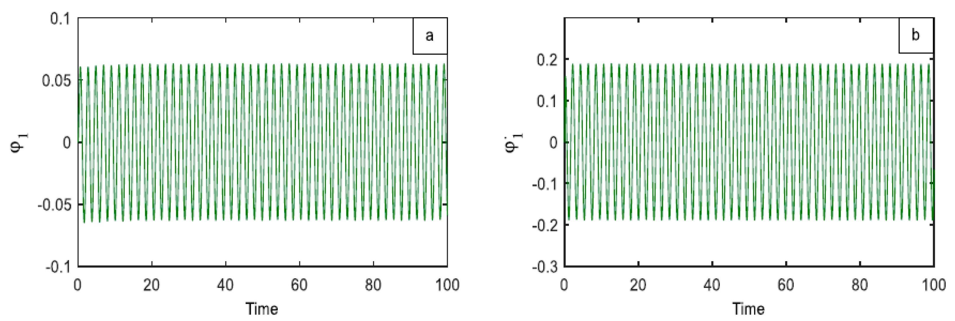
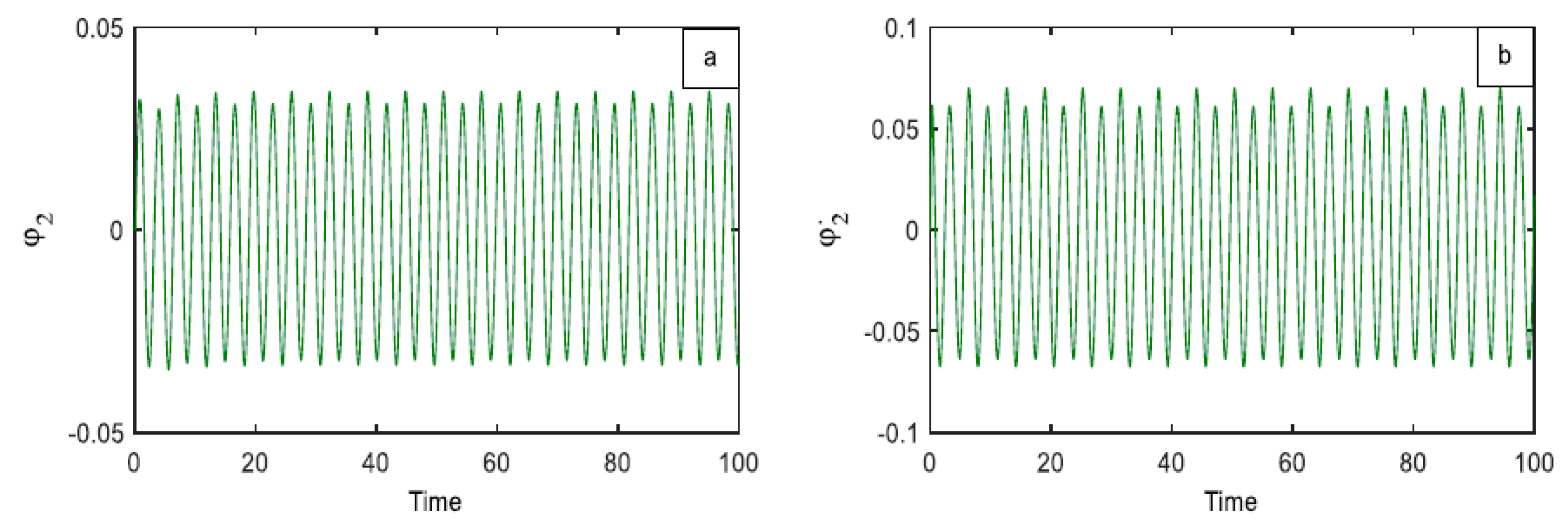
4.1. Time History Performance without Control

To analyze the behavior of the dynamical system the fourth-order Runge–Kutta algorithm (ode45 in MATLAB) [30] is applied to find the numerical solution of the given uncontrolled system of Equations (8) and (9).

The time history performance of the system without any controller at the primary resonance (${\mathsf{\Omega }}_1\cong {\omega }_1,{\mathsf{\Omega }}_2\cong {\omega }_2$) is shown in Figure 3 at the chosen values $({\omega }_1=3;\zeta =0.2;{\omega }_2=2;\beta =0.5{\omega }_2^2;{\alpha }_1=0.2;{\alpha }_2=0.3;f_1=10;{\alpha }_3=2{\alpha }_1;{\alpha }_4=2{\alpha }_2;$ $f_2=5;{\mathsf{\Omega }}_1={\omega }_1;{\mathsf{\Omega }}_2={\omega }_2)$.

Figure 3a,b show the steady-state time response against the amplitude ${\phi }_1$ for the uncontrolled first system and the velocity ${\dot{\phi }}_1$, respectively. Similarly, Figure 4a,b show the uncontrolled second main system and its amplitude ${\phi }_2$ and velocity ${\dot{\phi }}_2$ with the time response.

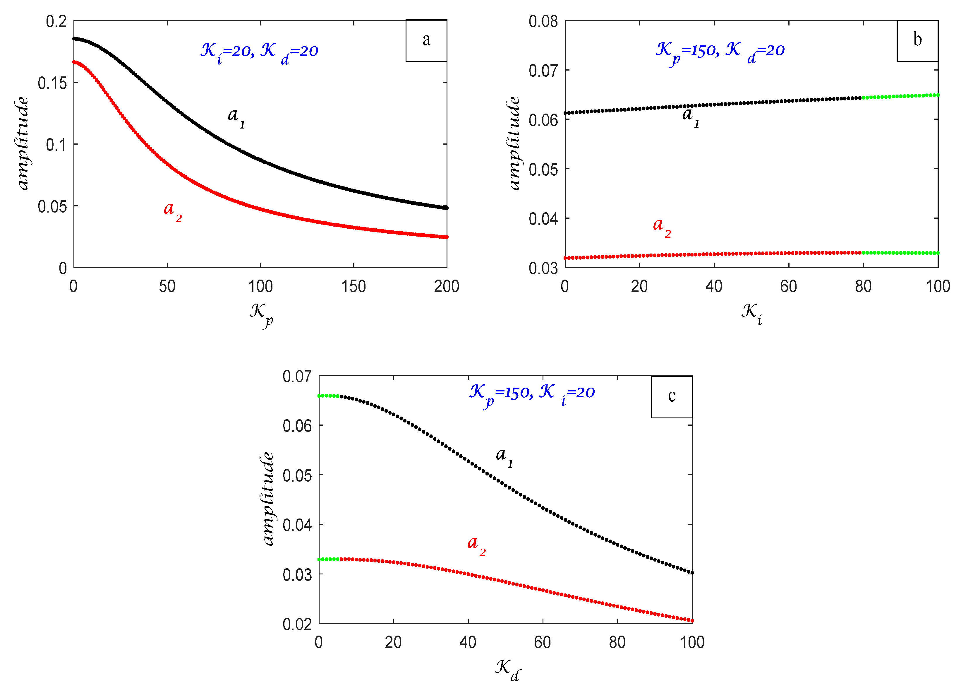
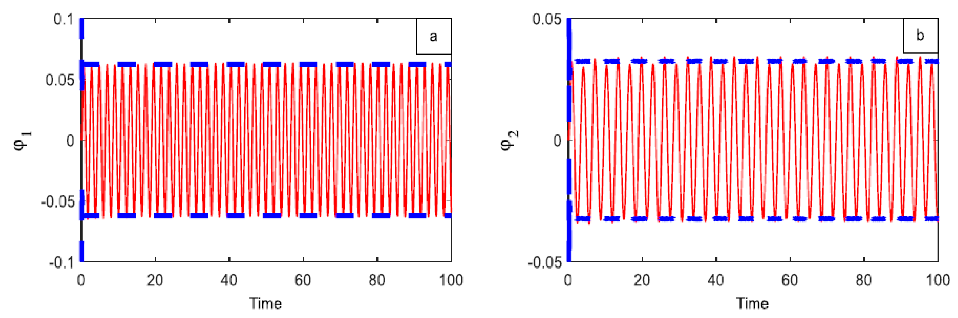
4.2. Time History Performance with Different Control

The closed-loop performances of the P, PI, and PID controllers for the two systems ${\phi }_1$ and ${\phi }_2$, along with their corresponding velocities ${\dot{\phi }}_1$ and ${\dot{\phi }}_2$, are displayed in Figure 5. The closed-loop responses of the traditional P and PI controllers are unstable and exhibit peak overshoot. Better closed-loop performance, such as in responses with less peak overshoot and settling time, was supplied by the redesigned PID controller structure, which conveys closed-loop responses with less peak and overshoot and a more stable curve than the others. The study was for the first main system and its velocity, as in Figure 5a,b, and the second main system shown in Figure 5c,d. Figure 5 shows evidence of both steady behavior and the absence of chaos in the produced wavelengths and amplitudes in every section. We utilized the gain values that are depicted in

Table 1. Parameters of a PID controller.

Controller		Gain
		$K_p$	$K_i$	$K_d$
P	(Red)	150	-	-
PI	(Blue)	150	20	-
PID	(Green)	150	20	20

to obtain these closed loops using the three control approaches.

In Figure 6a,b, there is a depiction of the first main system’s amplitude decreasing from 7.788 to 0.0569 after the utilization of a time PID controller. This indicates that the controller’s effectiveness ($E_a$ = amplitude without control/amplitude with) was equivalent to 136.87 for the first main system ${\phi }_1$, with a proportional reduction of 99.27%. Likewise, the amplitude ${\phi }_2$ of the second system, which is equal to 13.59, as shown in Figure 7, decreased to 0.02886, where $E_a$ = 470.89, reflecting a proportional reduction of 99.79%.

Figure 8 illustrates the phase plane of both main systems before and after adding the PID controller. Figure 8a shows that the first main system ${\phi }_1$, with a multi-limit cycle in the case of not adding control, and as improved with a limited cycle after adding PID. With the second main system ${\phi }_2$, as shown in Figure 8b before adding the control, the phase plane is the multi-limit cycle, which decreased after adding PID.

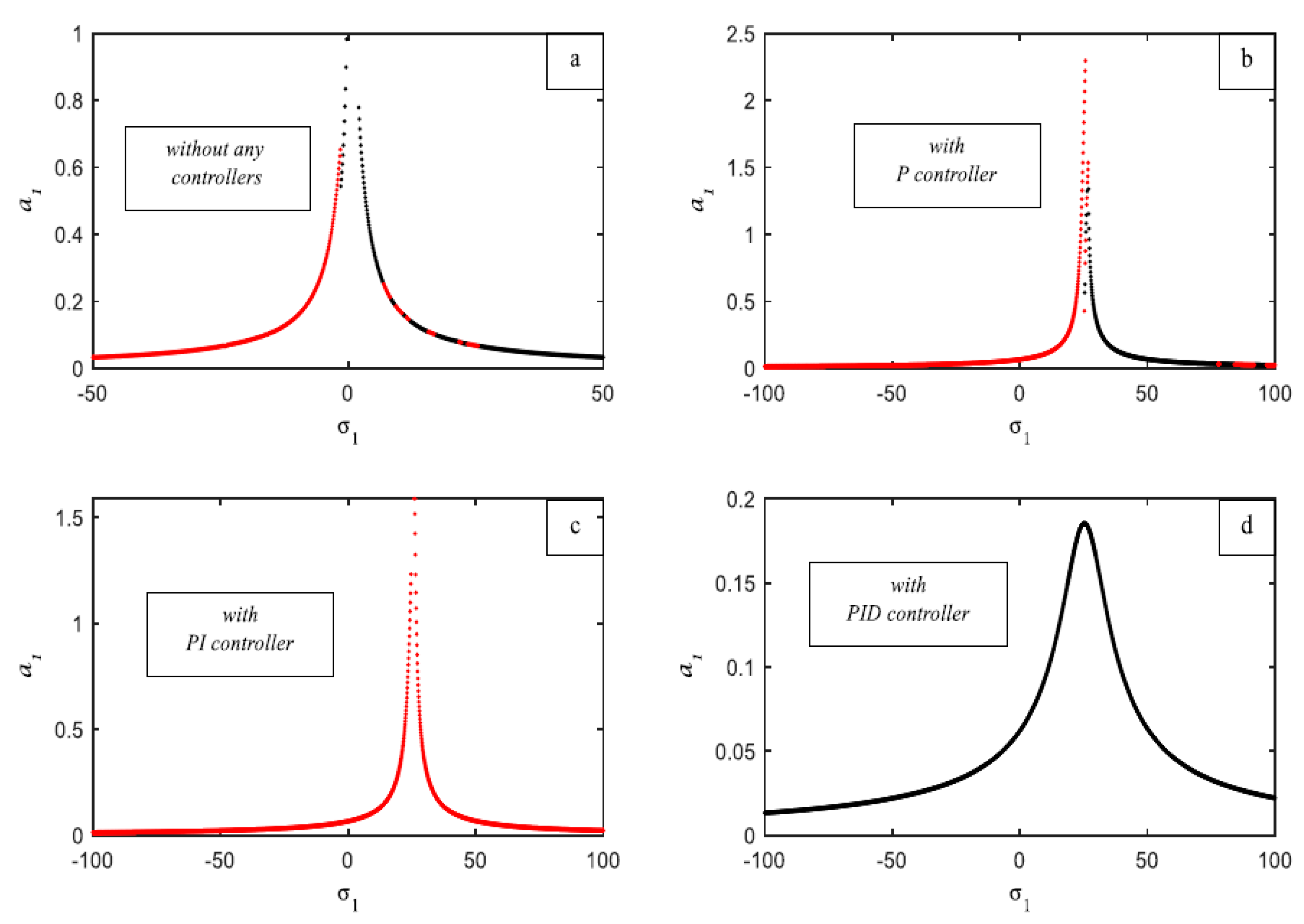
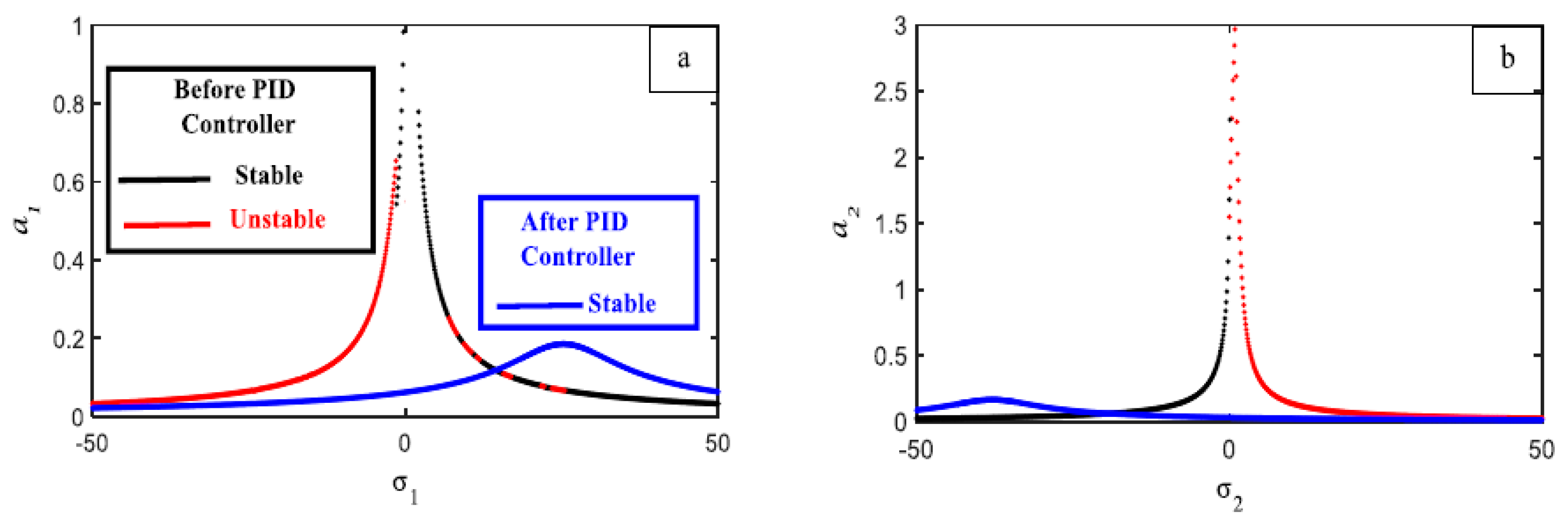
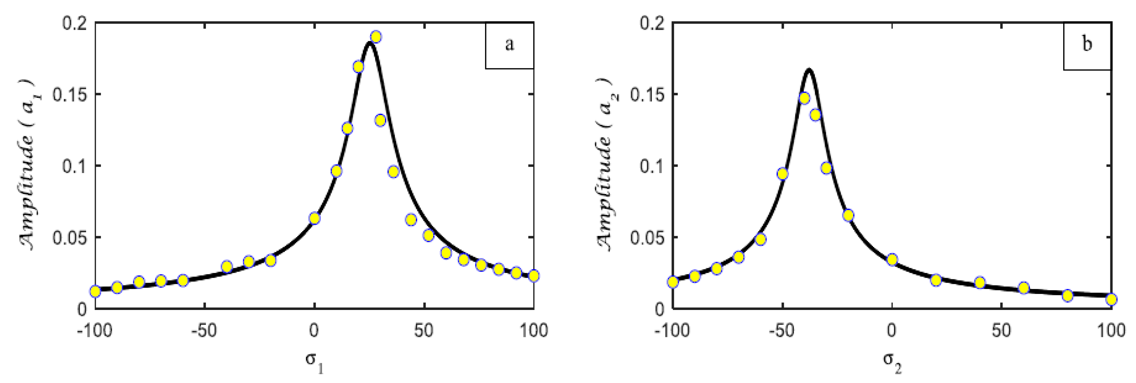
4.3. Frequency Response Curves (FRC)

The frequency response curves of Equations (32) and (33) of the first main system $a_1$, against the detuning parameter ${\sigma }_1$, are illustrated in Figure 9a without the influence of any controller, where the solid black line represents the stable solution while the red line indicates the unstable solution of the same equation. The amplitude of the first main system is fully reduced after the P controller is added; however, as Figure 9b shows, this declining portion of the curve is unstable. The response curve in Figure 9c shows what happens when a PI controller is added. It is discovered that this fully reduces the amplitude of the primary system $a_1$, yet the curve is absolutely unstable. After adding a PID controller, the first main system’s behavior is shown in Figure 9d, where it is discovered that the curve has a monotonically decreasing amplitude and is completely stable. The response curves of the second main system $a_2$, against the detuning parameter ${\sigma }_2$, are illustrated in Figure 10a without the influence of any controller. The amplitude of the second main system is fully reduced after the P controller is added; however, as Figure 10b shows, this declining portion of the curve is unstable. The response curve in Figure 10c shows what happens when a PI controller is added. It is discovered that this controller reduces the amplitude of the second system $a_2$, yet the curve behaves in an unstable way. After adding a PID controller, the second main system’s behavior is shown in Figure 10d, where it is discovered that the curve has a monotonically decreasing amplitude and is completely stable. Figure 11 clearly illustrates the difference in the curves’ responses before and after the PID controller was included for the two primary systems, $a_1$ and $a_2$. Figure 11a,b demonstrated how the system is only stable and does not contain any unstable parts, as well as how the addition of a PID controller causes the amplitude to drop with $a_1$ and disappear with $a_2$. The amplitude rose for increasing values of the external force $f_1$ for the first main system $a_1$, as Figure 12a illustrates, with the first component of the system, $a_1$. The amplitude of the first main system is shifted to the right and displays a monotonically declining curve as the values of natural frequency ${\omega }_1$ increase, as seen in Figure 12b.The amplitude decreases monotonically when the damping coefficient $\zeta$ values increase, as shown in Figure 12c. As the values of the nonlinear parameter $\beta$ increased, the amplitude of the first half of the system bent to the left, as illustrated in Figure 12d. Lastly, Figure 12e illustrates how the nonlinear parameter ${\alpha }_2$ behaves for both positive and negative parameter values. For very tiny negative values of ${\alpha }_2$, the curve bends left, but for high positive values of ${\alpha }_2$, the curve bends right. The second main system’s amplitude increased for large values of the external force $f_2$, as shown in Figure 13a, with the second portion of the system, $a_2$. As seen in Figure 13b, the second main system’s amplitude is moved to the right and exhibits a monotonic declining curve for increased values of the natural frequency ${\omega }_2$. As seen in Figure 13c, the amplitude remains constant and shifts to the right for extraordinarily high positive values of the nonlinear parameter ${\alpha }_4$ and to the left for extraordinarily low negative values of ${\alpha }_4$. The response of the gains with the amplitude is examined in Figure 14. Figure 14a establishes the values of $K_i$ and $K_d$. Upon further examination of the influence of $K_p$, we discovered that when $K_p$ values increase, the amplitude of both primary systems decreases while remaining steady. With different values of $K_i$, we observed that the amplitude of both main systems increased indistinguishably for the fixed values of $K_p$ and $K_d$. However, when $K_i=80$, both main systems behaved in an unstable manner, as shown in Figure 14b. Lastly, although the other two gains are fixed, Figure 14c shows the improvement of $K_d$. Painting made it evident that the amplitude is unstable at the initial $K_d$ values and that, in both systems, the amplitude decreases as $K_d$ increases.

5. Comparison

5.1. Comparison of the Perturbation’s Temporal Response Solutions with Numerical Techniques

Analytical solutions to Equations (29) and (30) are graphically represented by (---) lines, which correspond with the numerical solutions of Equations (13) and (14), as displayed in Figure 15a for the first main system, and in Figure 15b for the second main system.

5.2. Comparison between RK-4 and FRC

Figure 16 shows an acceptable agreement with the numerical solutions of Equations (4) and (5), using (RK-4) highlighted by yellow circles and the frequency response curves (FRC) for the two main systems $a_1$ in Figure 16a and $a_2$ in Figure 16b, which are presented with the solid line.

5.3. Comparison with Published Work

For previous work, the following can be stated:

(1)

Torsional vibration was examined in a review of the literature [25] for active and passive control, which is a useful tool for managing the torsional vibration of a nonlinear dynamical system that is exposed to several parametric excitations.

(2)

They used the frequency response equations; the stability of the system is examined in the vicinity of the simultaneous sub-harmonic and internal resonances.

(3)

The behavior of the system with and without two controllers is numerically integrated and examined.

For this work, after adding control, we compared the time histories of our work and a prior study and discovered that the amplitudes and wavelengths showed that the solutions generated exhibited stable behavior and were devoid of chaos.

6. Conclusions

The torsional vibration control of a nonlinear dynamical system has been tackled within this article. Proportional-integral-derivative (PID) controllers have been proposed to control the harmful torsional vibration of the system, as shown in Figure 2 for one of the worst resonance cases. The multiple-scale perturbation approach is applied to obtain the approximation solution for the coupled controlled system. The time history is drawn to study the steady-state vibration amplitudes and the effectiveness of the applied control algorithms in suppressing vibration. In addition, the stability and effects of different system and control parameters are illustrated in frequency response curves according to the Routh–Hurwitz criterion. Based on the above discussion, the following conclusions can be drawn:

(1)

It is noted that the PID controller is operated to reduce the dangerous vibrations in a short time.

(2)

This work provided a comparison between P, PI, and PID controllers in the context of FRCs.

(3)

Numerous coefficients’ effects are examined and shown numerically.

(4)

Despite the excitation frequency, the PID controller is the most effective control method for minimizing the vibrations in the framework.

(5)

The closed-loop response of relative displacement is obtained with the PID controller, which comprises the peak-overshoot.

(6)

The modified structure of the PID controller, such as with the P and PI controllers, is used for the control of the relative displacement of the suspension system. From the results, the PID controller provided better closed-loop performance in terms of peak overshoot and settling time, which are minimized.

References

1. Sowmya, V.S.; Dharsini, S.P.; Dharshini, R.P.; Aravind, P. Application of various PID controller tuning techniques for a temperature system. Int. J. Comput. Appl. 2014, 103, 32–34. [Google Scholar]
2. Pradeepkannan, D.; Sathiyamoorthy, S. Implementation of Gain Scheduled PID Controller for a Nonlinear Coupled Spherical Tank Process. Int. J. Mech. Mechatron. Eng. 2014, 14, 93–98. [Google Scholar]
3. Sabri, L.A.; Hussein, A.A. Implementation of fuzzy and PID controller to water level system using LabView. Int. J. Comput. Appl. 2015, 116, 6–10. [Google Scholar]
4. Bashiri, A.H. Empirical study of robust/developed PID control for nonlinear time-delayed dynamical system in discrete time domain. Heliyon 2024, 10, e29749. [Google Scholar] [CrossRef] [PubMed]
5. Hamed, A.; Shaban, E.M.; Darwish, R.R.; Abdel Ghany, A.M. Design and implementation of discrete PID control applied to Bitumen tank based on new approach of pole placement technique. Int. J. Dynam. Control 2017, 5, 604–613. [Google Scholar] [CrossRef]
6. Shaban, E.M.; Hamed, A.; Darwish, R.R.; Abdel Ghany, A.M. New tuning approach of discrete PI/PID controller applied to bitumen system based on non-minimal state space formulation. In Proceedings of the 25th International Conference on Computer Theory and Applications (ICCTA), Alexandria, Egypt, 24–26 October 2015; pp. 52–57. [Google Scholar]
7. Hamed, A.R.; Shaban, E.M.; Abdelhaleem, A.M. Industrial implementation of state dependent parameter PID+ control for nonlinear time delayed bitumen tank system. Iran J. Sci. Technol. Trans. Electr. Eng. 2022, 46, 743–751. [Google Scholar] [CrossRef]
8. Sayed, H.; Shaban, E.M.; Abdelhamid, A. State-Dependent Parameter PID+ Control Applied to A Nonlinear Manipulator Arm. In Recent Advances in Engineering Mathematics and Physics; Farouk, M., Hassanein, M., Eds.; Springer: Cham, Switzerland, 2020. [Google Scholar]
9. Dano, M.L.; Julli’ere, B. Active control of thermally induced distortion in composite structures using macro fiber composite actuators. Smart Mater. Struct. 2007, 16, 2315–2322. [Google Scholar] [CrossRef]
10. Kumar, R.S.; Ray, M.C. Active control of geometrically nonlinear vibrations of doubly curved smart sandwich shells using 1–3 piezoelectric composites. Compos. Struct. 2013, 105, 173–187. [Google Scholar] [CrossRef]
11. Saeed, N.; Kamel, M. Nonlinear PD-controller to suppress the nonlinear oscillations of horizontally supported Jeffcott-rotor system. Int. Non-Linear Mech. 2016, 87, 109–124. [Google Scholar] [CrossRef]
12. Fey, R.H.B.; Wouters RM, T.; Nijmeijer, H. Proportional and derivative control for steady-state vibration mitigation in a piecewise linear beam system. Nonlinear Dyn. 2010, 60, 535–649. [Google Scholar] [CrossRef]
13. Eissa, M.; Kandil, A.; El-Ganaini, W.A.; Kamel, M. Analysis of a nonlinear magnetic levitation system vibrations controlled by a time-delayed proportional derivative controller. Nonlinear Dyn. 2015, 79, 1217–1233. [Google Scholar] [CrossRef]
14. Eissa, M.; Kandil, A.; Kamel, M.; El-Ganaini, W.A. On controlling the response of primary and parametric resonances of a nonlinear magnetic levitation system. Meccanica 2015, 50, 233–251. [Google Scholar] [CrossRef]
15. Bauomy, H.S.; EL-Sayed, A.T. Act of nonlinear proportional derivative controller for MFC laminated shell. Phys. Scr. 2020, 95, 095210. [Google Scholar] [CrossRef]
16. Hote, Y.V.; Jain, S. PID controller design for load frequency control: Past, Present and future challenges. IFAC-Pap. Online 2018, 51, 604–609. [Google Scholar] [CrossRef]
17. Darwish, N.M. PID controller design in the frequency domain for time-delay systems using direct method. Trans. Inst. Meas. Control 2018, 40, 940–950. [Google Scholar] [CrossRef]
18. Zhao, C.; Guo, L. PID controller design for second order nonlinear uncertain systems. Sci. China Inf. Sci. 2017, 60, 022201. [Google Scholar] [CrossRef]
19. Hanafi, D. PID controller design for semi-active car suspension based on model from intelligent system identification. In Proceedings of the IEEE Computer Society, Second International Conference on Computer Engineering and Applications, Bali, Indonesia, 19–21 March 2010; pp. 60–63. [Google Scholar]
20. Constantin, M.; Popescu, O.S.; Mastorakis, N.E. Testing and simulation of motor vehicle suspension. Int. J. Syst. Appl. Eng. Dev. 2009, 3, 74–83. [Google Scholar]
21. Kumar, M.S. Development of Active System for Automobiles using PID Controller. In Proceedings of the World Congress on Engineering, London, UK, 2–4 July 2008; Volume II. [Google Scholar]
22. Govinda, K.E.; Raghul, S.; Kishore, K.R.; Mathan, K.M.; Prasanth, C. Enhancing the Closed Loop Performance of Semi-active Suspension System with I-PD Controller. Mater. Sci. Eng. 2019, 561, 012085. [Google Scholar] [CrossRef]
23. Amer, Y.A.; EL-Sayed, A.T.; El-Bahrawy, F.T. Torsional vibration reduction for rolling mill’s main drive system via negative velocity feedback under parametric excitation. J. Mech. Sci. Technol. 2015, 29, 1581–1589. [Google Scholar] [CrossRef]
24. Wenzhi, G.; Zhiyong, H. Active control and simulation test study on torsional vibration of large turbo-generator rotor shaft. Mech. Mach. Theory 2010, 45, 1326–1336. [Google Scholar] [CrossRef]
25. El-Sayed, A.T.; Bauomy, H.S. Passive and active controllers for suppressing the torsional vibration of multiple degree-of-freedom system. J. Vib. Control 2015, 21, 2616–2632. [Google Scholar] [CrossRef]
26. Jianhui, W.; Yushen, W.; Philip Chen, C.L.; Zhi, L.; Wenqiang, W. Adaptive PI event-triggered control for MIMO nonlinear systems with input delay. Inf. Sci. 2024, 677, 120817. [Google Scholar]
27. Yang, W.W.; Yang, Y.J.; Tang, X.Y.; Zhang, K.R.; Li, J.C.; Xu, C. An adaptive P/PI control strategy for a solar volumetric methane/steam reforming reactor with passive thermal management. Chem. Eng. Sci. 2023, 281, 119005. [Google Scholar] [CrossRef]
28. Kevorkian, J.; Cole, J.D. Multiple Scale and Singular Perturbation Methods. In Applied Mathematical Sciences; Springer: Berlin/Heidelberg, Germany, 1996. [Google Scholar]
29. Nayfeh, A. Perturbation Methods; Wiley: New York, NY, USA, 1973. [Google Scholar]
30. Dukkipati, R.V. Solving Vibration Analysis Problems Using Matlab; New Age International Pvt Ltd Publishers: New Delhi, India, 2007. [Google Scholar]
31. Bauomy, H.S.; El -Sayed, A.T. Mixed controller (IRC+ NSC) involved in the harmonic vibration response cantilever beam model. Meas. Control 2020, 53, 1954–1967. [Google Scholar] [CrossRef]
32. Kamel, M.; Eissa, M.; El-sayed, A.T. Vibration reduction of a nonlinear spring pendulum under multi-parametric excitation via a longitudinal absorber. Phys. Scr. 2009, 80, 025005. [Google Scholar] [CrossRef]
33. Bauomy, H.S.; El -Sayed, A.T.; Salem, A.M.; El-Bahrawy, F.T. The improved giant magnetostrictive actuator oscillations via positive position feedback damper. AIMS Math. 2023, 8, 16864–16886. [Google Scholar] [CrossRef]
34. Bauomy, H.S.; El -Sayed, A.T.; El-Bahrawy, F.T.; Salem, A.M. Safety of a continuous spinning Shaft’s structure from nonlinear vibration with NIPPF. Alex. Eng. J. 2023, 67, 193–207. [Google Scholar] [CrossRef]
35. Bauomy, H.S.; El -Sayed, A.T. Vibration performance of a vertical conveyor system under two simultaneous resonances. Arch. Appl. Mech. 2018, 88, 1349–1368. [Google Scholar] [CrossRef]
36. El-Sayed, A.T.; Bauomy, H.S. NIPPF versus ANIPPF controller outcomes on semi- direct drive cutting transmission system in a shearer. Chaos Solitons Fractals 2022, 156, 111778. [Google Scholar] [CrossRef]
37. Forming Equations of Motion for Multiple Degree-of-Freedom Systems. Available online: www.efunda.com/formulae/vibrations/mdof_eom.cfm (accessed on 1 January 2013).
Figure 1. Model of schematic diagram of main system.
Computation 12 00157 g001
Figure 2. Model of schematic diagram of main system with PID controllers.
Computation 12 00157 g002
Figure 3. The time diagram without any controller (a) the first part of the system, φ 1 (b) the response of its velocity, φ ˙ 1 .
Computation 12 00157 g003
Figure 4. The time diagram without any controller (a) the second part of the system, φ 2 (b) response of its velocity, φ ˙ 2 .
Computation 12 00157 g004
Figure 5. Responses in closed loop using P, PI, and PID controller. (a) the first part of the system φ 1 (b) the response of its velocity φ ˙ 1 (c) the second part of the system φ 2 (d) the response of its velocity φ ˙ 2 .
Computation 12 00157 g005
Figure 6. The time diagram in the primary resonance situation with the PID controller (a) the first part of the system φ 1 (b) the response of its velocity φ ˙ 1 .
Computation 12 00157 g006
Figure 7. The time diagram in the primary resonance situation with the PID controller (a) the second part of the system φ 2 (b) the response of its velocity φ ˙ 2 .
Computation 12 00157 g007
Figure 8. The phase plane of the system’s (a) φ 1 with angular velocities φ ˙ 1 in the primary resonance situation without control (b) φ 1 with angular velocities φ ˙ 1 in the primary resonance situation with the PID controller (c) φ 2 with angular velocities φ ˙ 2 in the primary resonance situation without control (d) φ 2 with angular velocities φ ˙ 2 in the primary resonance situation with the PID controller.
Computation 12 00157 g008
Figure 9. The frequency response curves on the plane σ 1 and the first part of the system ( a 1 ) (a) without a controller, (b) with a P controller, (c) with a PI controller, and (d) with a PID controller. (red color) unstable region (black color) stable region
Computation 12 00157 g009
Figure 10. The frequency response curves on plane σ 2 and the first part of the system ( a 2 ) (a) without a controller, (b) with a P controller, (c) with a PI controller, and (d) with PID controller. (red color) unstable region (black color) stable region.
Computation 12 00157 g010
Figure 11. Frequency response before and after PID: (a) first main system a 1 and (b) first main system a 2 .
Computation 12 00157 g011
Figure 12. (a) The FRC of the external force action f 1 . (b) Natural frequency ω 1 . (c) Damping coefficient ζ . (d) Linear parameter β . (e) Nonlinear parameter α 2 . All of these regard the first part of the system a 1 .
Computation 12 00157 g012aComputation 12 00157 g012b
Figure 13. (a) The FRC of the external force action f 2 . (b) Natural frequency ω 2 . (c) Nonlinear parameter α 4 . All of these regard the second part of system a 2 .
Computation 12 00157 g013
Figure 14. Response curve for the system amplitudes with (a) K p (b) K i (c) K d .
Computation 12 00157 g014
Figure 15. Comparison of numerical simulation and perturbation analysis for both framework modes in PID controllers. (a) the first part of the system φ 1 (b) the second part of the system φ 2
Computation 12 00157 g015
Figure 16. Contrast between the FRC solution and RK- 4 solution for both systems (a) the first part of the system a 1 (b) the second part of the system a 2 .
Computation 12 00157 g016