Analogue Computation Converter for Nonhomogeneous Second-Order Linear Ordinary Differential Equation

Abstract

Among many other applications, electronic converters can be used with sensors with analogue outputs (DC voltage). This article presents an analogue computation converter with two DC voltages at the inputs (one input changes the frequency of the output signal, another input changes the amplitude of the output signal) that provide a periodic sinusoidal signal (with variable frequency and amplitude) at the output. On the basis of the analogue computation converter is a nonhomogeneous second-order linear ordinary differential equation which is solved analogically. The analogue computation converter consists of analogue multipliers and operational amplifiers, composed of seven function circuits: two analogue multiplication circuits, two analogue addition circuits, one non-inverting amplifier, and two integration circuits (with RC time constants). At the output of an oscillator is a sinusoidal signal which depends on the DC voltages applied on two inputs (0 ÷ 10 V): at one input, a DC voltage is applied to linearly change the sinusoidal frequency output (up to tens of kHz, according to two time constants), and at the other input, a DC voltage is applied to linearly change the amplitude of the oscillator output signal (up to 10 V). It can be used with sensors which have a DC output voltage and must be converted to a sine wave signal with variable frequency and amplitude with the aim of transmitting information over longer distances through wires. This article presents the detailed theory of the functioning, simulations, and experiments of the analogue computation converter.

1. Introduction

Sinusoidal oscillators are essentially non-linear systems (this is the reason for their stable amplitude) and have been shown to be useful in many applications, these include sensors, measuring systems, telecommunications, control systems, and analogue signal processing. The oscillation circuits can be LC oscillators, RC oscilators, voltage-controlled oscillators, quartz crystal oscillators, phase shift oscillators, Wien- and Colpitts-type oscillators, and others (with frequency of hundreds of kHz). This type of oscillator can be used to design other types of oscillators, such as voltage-controlled crystal oscillators, quartz resonator sensors, digitally programmable voltage (current)-controlled oscillators, CMOS sinusoidal oscillators by using operational transconductance amplifier–capacitor, etc. [1,2,3,4,5,6,7,8].

The structures of voltage–frequency converters that are designed for measuring DC voltages with slow variation or that have electronic switches in their structure, with a rectangular signal on the output and two-stage measurement, are well known. Their disadvantage is the high response speed when rapidly changing the input voltage and limiting the transmission of the signal over long distances. At the same time, the structures of voltage–frequency converters that have reference oscillators, counters, and digital-to-analogue converters are known, as well as the structure of converters with resonant and feedback networks and derivation and amplification circuits. Their disadvantages are that the output signal can change in a limited range, their structure is complicated, the response speed is high, and the signal is non-sinusoidal. Because they have a dependable start-up and low sensitivity, electronic oscillators (with sinusoidal or other forms of signals, such as rectangular) can be utilized in applications using resistive and capacitive sensors [9,10,11,12]. The oscillators’ main function is to change the frequency and amplitude of the output signals [8,9,10,13,14,15,16].

Oscillators are essential circuit-building blocks in electronic apparatus (instrumentation), serving as timekeeping references, clock sources, and excitation sources, among other things. Oscillators are used in wave signal generation, filters, transducer circuits, carrier amplifiers, generators, and data converters. Although many techniques are widely used, a simple, accurate, and tunable oscillator has yet to be developed [13,17]. Many sinusoidal oscillator circuits (with bipolar or field transistors or with linear circuits as an active element) are accessible in the literature, with design guidelines, characteristic equations, and analysis provided for most applications. They work in the same way as sinusoidal oscillators [3,18,19,20,21,22,23,24,25]. The Barkhausen stability criterion, used for sustained oscillation, states that the gain around the loop, composed by the amplifier and phase shift network and the phase shift around the loop, is 360° or 0° [22,26]. There are articles that present an original oscillator circuit with a structure that allows no electronic control and has mutually dependent conditions and oscillation frequency utilizing a electronically regulated second-generation current conveyor [27].

With the resistance-controlled, capacitor-controlled, or tunable high-frequency oscillators, they were made into simple digitally programmable voltage (current)-controlled oscillators with a grounded capacitor, an operational amplifier, two operational transconductance amplifiers, and one fixed DC power supply that produce a signal of hundreds of kHz at the output for input voltages up to 10 V [1,28,29].

The construction of quicker and more efficient communication systems is motivated by the rapid development of communications for numerous applications with a large number of users. Due to estimation mistakes and hardware limitations, real-time communication systems perform below capacity constraints (e.g., oscillator phase noise and the level of phase noise). Oscillators are utilized for frequency shifting in communications, while voltage-controlled oscillators are employed for modulation and detection [23,24,25,30,31].

In many applications (e.g., medical), sinusoidal oscillators with low total harmonic distortion (e.g., digital–harmonic-cancellation structure, designed by summing up a set of square wave signals with different phase shifts and different summing coefficients to cancel unwanted harmonics) are used, and generated sinusoidal signals should be tunable (within the frequency range from 10 kHz to 10 MHz) [32]. A single-phase current-source inverter (with a linear amplifier, such as a class-A or class-D type) that generates a pure sinusoidal waveform with little switching losses and employs a small-size output filter capacitor with small ripples at the output was created in earlier publications [9].

Capacity measurements from various sensors (accelerometers, liquid-level gauges, pressure, etc.), which usually have low values of the output capacity (dozens of pF), can be used to measure the noise performance of a capacitive–sensor interface with a simple relaxation oscillator, a fast counter, and a microcontroller. Such a measurement time can be acceptable for measurement systems with slow-changing physical signals. The noise performance of a capacitive–sensor interface with a simple relaxation oscillator, a fast counter, and a microcontroller can be evaluated using capacity measurements from a capacitive–sensor interface with a simple relaxation oscillator, a fast counter, and a microcontroller. Such a measurement interval may be appropriate for measurement systems with slow-changing physical signals [20].

Capacitive-coupling impedance spectroscopy utilizing a non-sinusoidal oscillator and discrete-time Fourier transform may be employed with other equipment devices (such as those used in spectroscopy) [33].

An amplitude-limiting mechanism can usually be created with operational transconductance amplifier nonlinearity in an analogue sinusoidal oscillator. In sensors, instrumentation systems, and communication systems, the sinusoidal oscillator is a basic analogue–circuit component. The LC structure can be utilized to create high-quality oscillators (used in radio frequency systems) but cannot practically be realized in integrated circuits. Other types of oscillators, such as ring oscillators, are compact in size but have a large harmonic content, which limits them [34,35,36,37,38].

Starting with a fundamental equation utilized in automation: the second order differential equation with constant coefficients, this article provides a variable frequency oscillator signal generated with an analogue computer (constructed with analogue blocks of multiplication, addition, amplification, and integration). This article has the following structure: mathematical modelling, analogue computation converter simulation, experimentation, discussions, and conclusions.

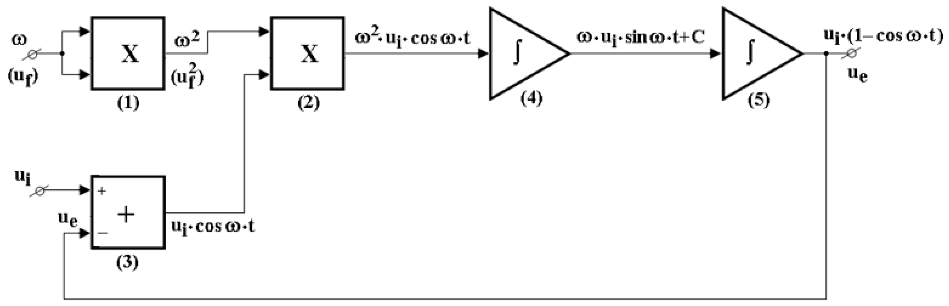
2. Mathematical Model

It is a well-known second-order linear ordinary differential equation that is used in electrical engineering, electronics, and automation (among other things):

$$a_2·{\displaystyle \frac{d^{2}y\left(t\right)}{{dt}^2}}+a_1·{\displaystyle \frac{dy\left(t\right)}{dt}}+a_0·y(t)=b_0·x(t)$$

(1)

where a₂, a₁, a₀, and b₀ are parameters, and y(t) and x(t) are functions depending on time. Equation (1) can be written as follows:

$${\displaystyle \frac{a_2}{a_0}}·{\displaystyle \frac{d^{2}y\left(t\right)}{{dt}^2}}+{\displaystyle \frac{a_1}{a_0}}·{\displaystyle \frac{dy\left(t\right)}{dt}}+y(t)={\displaystyle \frac{b_0}{a_0}}·x(t)$$

(2)

If it is noted that:

$$\omega =\sqrt{{\displaystyle \frac{a_0}{a_2}}};\xi ={\displaystyle \frac{a_1}{2}}{\displaystyle \frac{1}{\sqrt{a_0·a_2}}};K_s={\displaystyle \frac{b_0}{a_0}}$$

(3)

where ω is natural frequency, $\xi$ is the damping ratio, and K_s is the gain, then the Equation (2) becomes the following:

$${\displaystyle \frac{1}{{\omega }^2}}·{\displaystyle \frac{d^{2}y\left(t\right)}{{dt}^2}}+{\displaystyle \frac{2·\xi }{\omega }}·{\displaystyle \frac{dy\left(t\right)}{dt}}+y(t)=K_s·x(t)$$

(4)

If K_s = 1, then Equation (4) becomes the following:

$${\displaystyle \frac{d^{2}y(t)}{{dt}^2}}+2·\xi ·\omega ·{\displaystyle \frac{dy\left(t\right)}{dt}}+{\omega }^2·y(t)={\omega }^2·x(t)$$

(5)

which is nonhomogeneous second-order linear ordinary differential equation [39,40].

If it is considered that x(t) = 0, then Equation (5) becomes a homogeneous linear equation that has a natural response:

$${\displaystyle \frac{d^{2}y(t)}{{dt}^2}}+2·\xi ·\omega ·{\displaystyle \frac{dy\left(t\right)}{dt}}+{\omega }^2·y\left(t\right)=0$$

(6)

Roots of Equation (6) are as follows:

$$y\left(t\right)={\alpha }_1·e^{s_1·t}+{\alpha }_2·e^{s_2·t}$$

(7)

where

$$s_{\mathrm{1,2}}=-\xi ·\omega \pm \omega ·\sqrt{{\xi }^2-1},$$

(8)

α₁ and α₂ are two coefficients.

For the roots of Equation (6) and ξ > 0, there are four situations, depending on the value of ξ (Figure 1):

–

If $\xi$ > 1 y(t) has the roots (8) (real and distinct roots), and y(t) has an underdamped response;

–

If $\xi$ = 1 x(t) has the roots $s_{\mathrm{1,2}}=-\omega$ (real equal roots), and y(t) has a critical underdamped response;

–

If $\xi$ < 1 x(t) has the roots $s_{\mathrm{1,2}}=-\xi ·\omega \pm j·\omega ·\sqrt{1-{\xi }^2}$ (complex conjugate roots), and y(t) has a critical overdamped response with damped oscillation.

–

If $\xi$ = 0, x(t) has the roots $s_{\mathrm{1,2}}=\pm j·\omega$ (imaginary conjugate roots), and the response will be oscillation (without damped oscillation). In a real oscillator, the first root is useful for making oscillations: $s_1=+j·\omega$. This variant is the basis of the realization of the analogue computation converter.

In Figure 1, the sizes on the horizontal and vertical axes are principle sizes.

Returning to Equation (5) and setting, the condition ξ = 0 is obtained as follows:

$${\displaystyle \frac{d^{2}y(t)}{{dt}^2}}+{\omega }^2·y(t)={\omega }^2·x(t)$$

(9)

which is a particular case of the un-homogeneous Equation (5), and the root of the Equation (9) is as follows:

$$s_{\mathrm{1,2}}=S_r+{\alpha }_1·e^{s_1·t}+{\alpha }_2·e^{s_2·t}$$

(10)

where S_r is the specific root of nonhomogeneous equation.

Starting from Equation (5) and considering that y(t) = u_e(t), ω is proportional to u_f(t) with constant $\sqrt{k}$, and x(t) = u_i(t), where u_f(t) and u_i(t) are DC voltages (varying slowly over time), it is written as follows:

$${\displaystyle \frac{d^2{u}_e(t)}{{dt}^2}}+2·\xi ·\omega ·{\displaystyle \frac{d{u}_e(t)}{dt}}+{\omega }^2·u_e(t)={\omega }^2·u_i(t)$$

(11)

Using the fundamental equation, in order to obtain an undamping oscillating regime at the output of the circuit, the condition in the above relation is put as ξ = 0. This relationship develops into the following:

$${\displaystyle \frac{d^2{u}_e(t)}{{dt}^2}}={\omega }^2·\left[u_i(t)-u_e(t)\right]$$

(12)

or

$${\displaystyle \frac{d^2{u}_e(t)}{{dt}^2}}=k·u_f^2(t)·\left[u_i(t)-u_e(t)\right]$$

(13)

A specific root to the above equation is found under certain circumstances:

$$u_e(t)=u_i(t)·\left(1-cos\omega t\right)$$

(14)

So, using analogue electronic circuits (actually, building an analogue computer [41]) with two inputs u_f and u_i, DC voltage) and one output (u_e, sinusoidal voltage with controlled frequency and amplitude), a sinusoidal signal can be obtained at the output from a DC signal u_f, which is proportional to the pulsation ω. At the same time, the amplitude of the output signal from another input can be changed (u_i, DC voltage).

With the help of five functional blocks, Figure 2 depicts the theoretical implementation of the above Equation (12) using analogue electrical circuits. This equation can theoretically be solved using two multiplication circuits ((1) and (2) blocks), an adding circuit ((3) block), and two integrating circuits ((4) and (5) blocks). Pulsation (ω), also in the equation, is implemented in the form of a DC voltage, u_f. This voltage can be adjusted to modify the frequency of the output signal. From u_i, the peak-to-peak amplitude of the output signal is changed.

The voltage at the input u_f is directly proportional to the frequency of the output signal f_e:

$$f_e={\displaystyle \frac{l}{2·\pi ·\sqrt{T_{i1·}{T}_{i2}}}}·u_f$$

(15)

where l is a proportionality constant, and T_i1 and T_i2 are the integration constants of the integration circuits.

The electrical oscillations whose amplitudes remain constant with time are called undamped oscillations. The frequency of the undamped oscillations remains constant. A voltage-controlled oscillator (VCO) is defined as an oscillator whose output frequency is controlled by an input voltage. The frequency of a VCO is directly proportional to the control voltage, meaning that as the input voltage increases, the frequency increases. VCOs can be harmonic oscillators, which produce sinusoidal waveforms, or relaxation oscillators, which produce sawtooth waveforms. Most VCOs have one DC input and one output frequency (

Table 1. Types of undamped sinusoidal oscillators.

Types of Undamped Sinusoidal Oscillators	Characteristics	Advantages	Disadvantages
Tuned Circuit Oscillators	These oscillators use a tuned circuit consisting of inductors and capacitors and are used to generate high-frequency (radio frequency) signals. Such oscillators are Hartley, Colpitts, and Clapp oscillators, etc.	– Periodic electronic signals such as a sine wave (or) a square wave; – Precise frequency generation; – Tunability; – Low phase noise.	– Noise; – Flexibility is poor; – High cost.
RC Oscillators	These oscillators use resistors and capacitors and are used to generate low- or audio-frequency signals. Thus, they are also known as audio-frequency oscillators. Such oscillators are Phase-shift and Wein-bridge oscillators.	– It is useful for frequencies in the audio range. – Simplicity of the circuit; – Wide range of frequency; – Distortion free; – Do not require any negative feedback and stabilization.	– It does not realize sine wave; – Takes a long start-up time; – The output is small because of the smaller feedback; – The RC phase shift oscillator requires high Vcc; – Poor frequency stability.
Crystal Oscillators	These oscillators use quartz crystals to generate highly stabilized output signal with frequencies up to 10 MHz. The Piezo oscillator is an example of a crystal oscillator.	– Signal quality of the crystal oscillator is good; – Stability; – Simple connection.	– Signal level is fixed; – Flexibility is poor; – The price is high; – Has a long start-up time.
Negative-resistance Oscillator	These oscillators use the negative-resistance characteristic of the devices such as tunnel devices. A tuned diode oscillator is an example of a negative-resistance oscillator.	– High-speed operation; – Low power consumption; – High sensitivity; – High efficiency.	– Limited voltage range; – Sensitive to temperature changes; – Limited current capacity.
Analogue computation converter	Using analogue electronic circuits with two DC inputs and one output (sinusoidal voltage with controlled frequency and amplitude). It is an analogue computer that solves a nonhomogeneous second-order linear ordinary differential equation.	– It has a DC input from which the frequency of the output signal is changed; – It has a DC input from which the amplitude of the output signal is changed; – The output signal is sinusoidal; – It can be used with analogue sensors to transmit information at a distance through electrical lines; – Stability; – Has a shot start-up time.	– Frequency in the range of kHz up to tens of kHz; – It has a relatively large number of passive components; – It is not stable for a wide range of input voltages.

) [3,4,5,13,22,23].

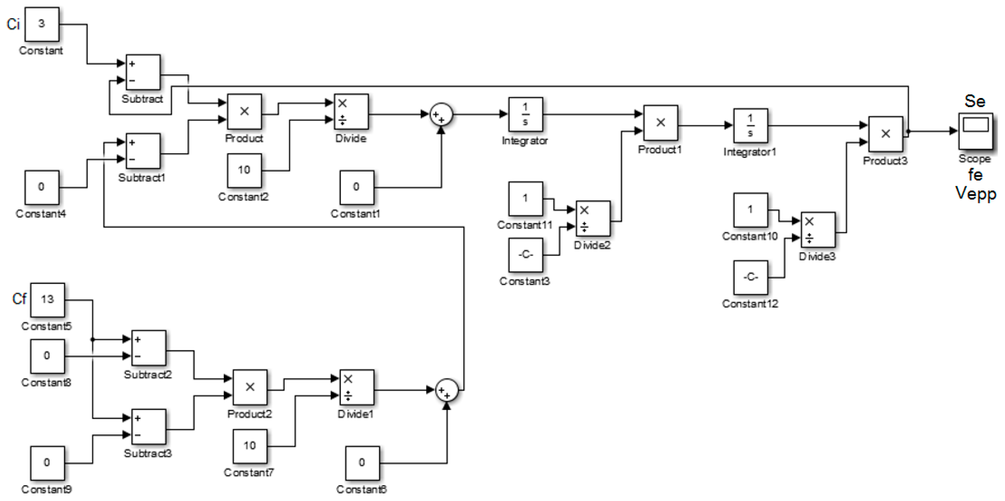
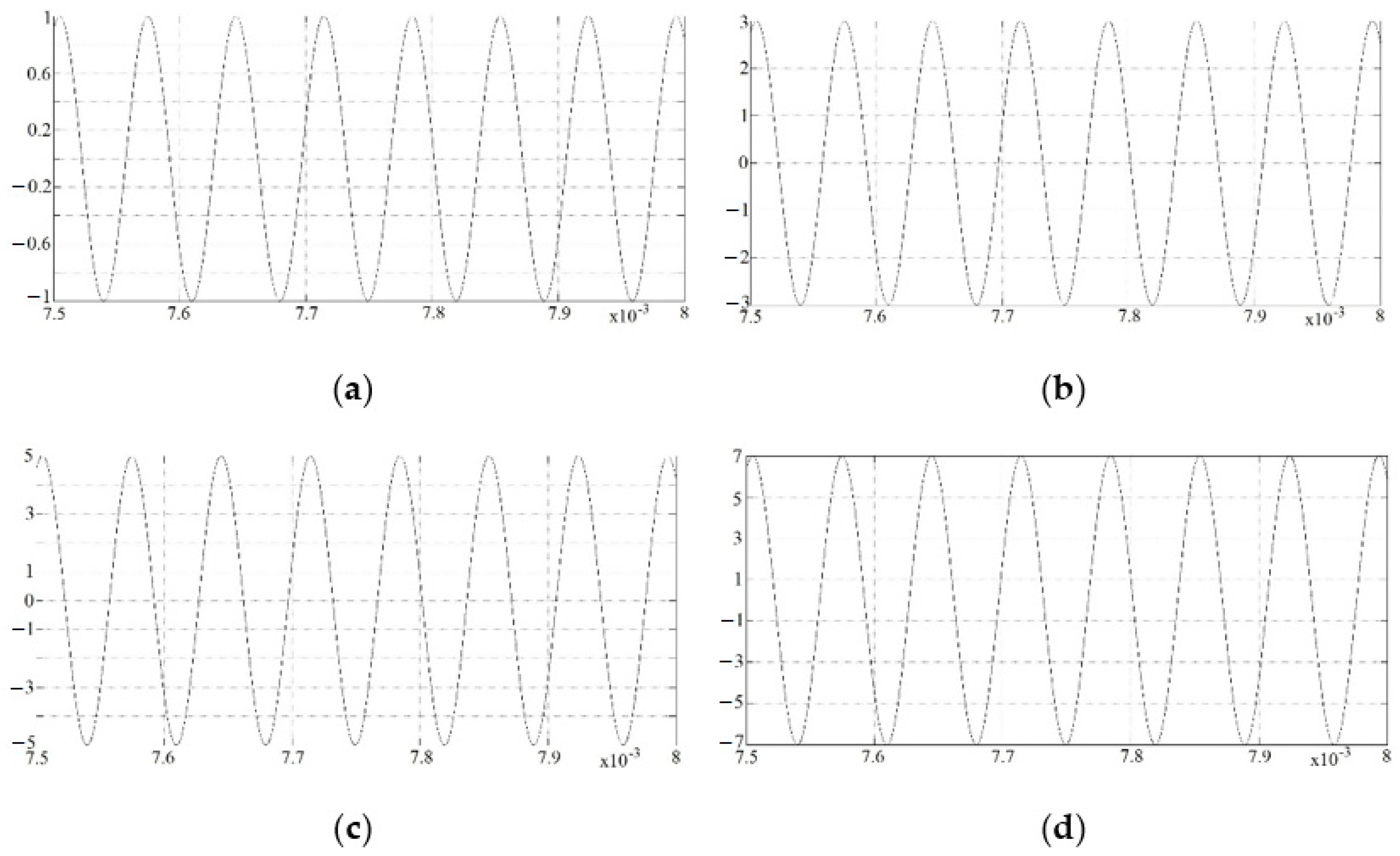
3. Simulations of an Analogue Computation Converter with Variable Frequency and Amplitude

Simulations were run using the Simulink module from Matlab R2014 to find the root to the nonhomogeneous second-order linear ordinary differential. Simulating the operation of the analogue converter, which is the basis of this sinusoidal oscillator with variable frequency and amplitude, verifies it at the same time. Using the blocks with constants, subtraction, multiplication, division, integration, and virtual output oscilloscope (Scope), the structure of the differential Equation (13) was observed. In Figure 3, the constants (on the left side of the figure) C_i, C_f (which simulate the DC voltages at input u_i and u_f) are mathematical quantities proportional to u_i (which determines the amplitude of the output signal u_s) and ω (which determines the frequency of the output signal u_e), and at the output, there will be a signal S_e (frequency f_e and peak-to-peak amplitude V_ppe, on the right side of Figure 3).

The operation of the analogue computation converter with changeable frequency and amplitude was verified by several simulations (Figure 4, Figure 5 and Figure 6).

The first set of simulations (Figure 4) were run with constant C_i (constant output signal amplitude) and varied C_f (which modifies the frequency of the output signal). The output signal is sinusoidal, the amplitude is constant, and the frequency changes linearly with C_f, according to the simulations.

The second set of simulations (Figure 5 and Figure 6) was run with varied C_i (changing output signal amplitude) and constant C_f (constant frequency of the output signal). The output signal is sinusoidal, the amplitude changes linearly as a function of C_i, and the frequency is constant, according to the simulations. Of course, regardless of the values of the constants C_i and C_f, the output of the theoretical analogue computation converter with variable frequency and amplitude produces an undamped sinusoidal signal (Figure 3).

Based on all simulations, the operating mode is not damped oscillating, with the output signal amplitude maintaining constant.

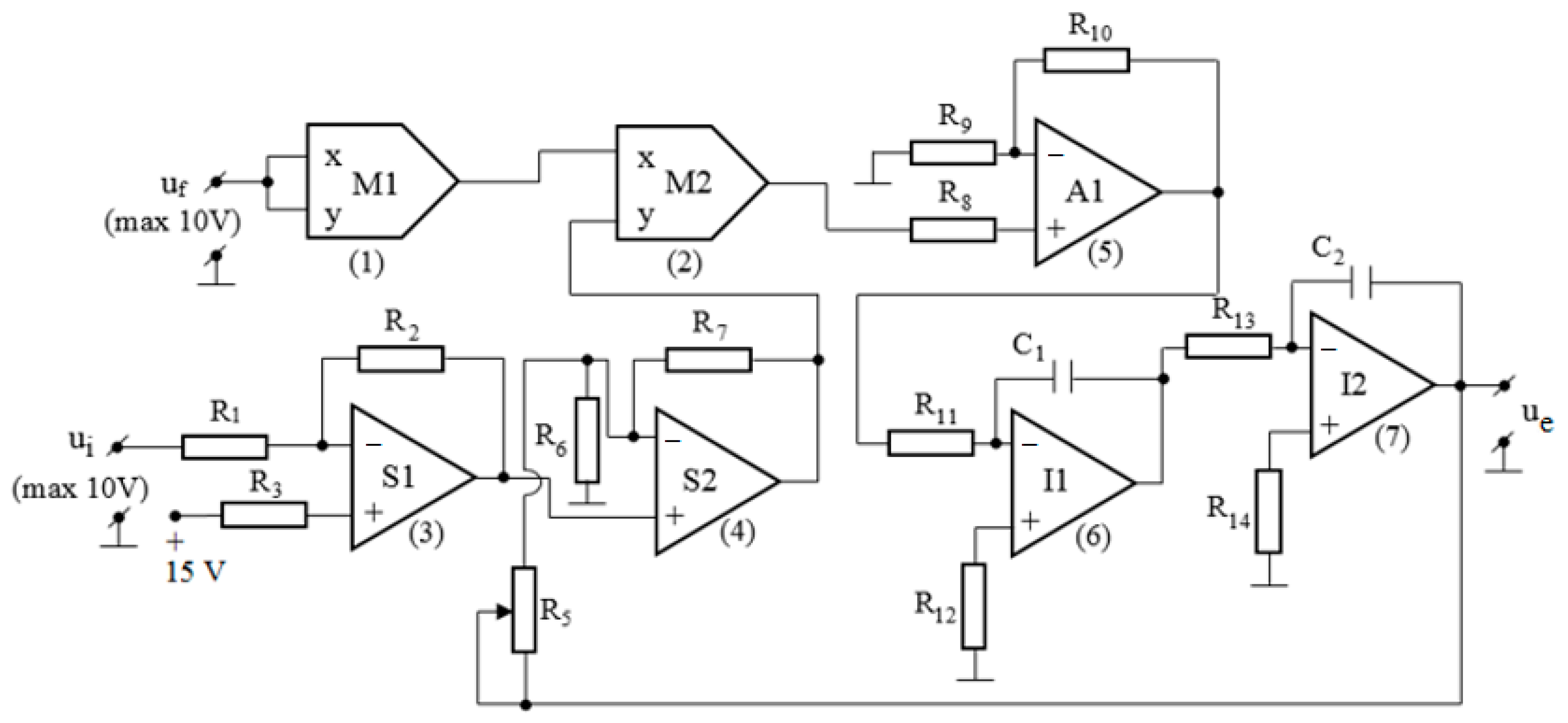
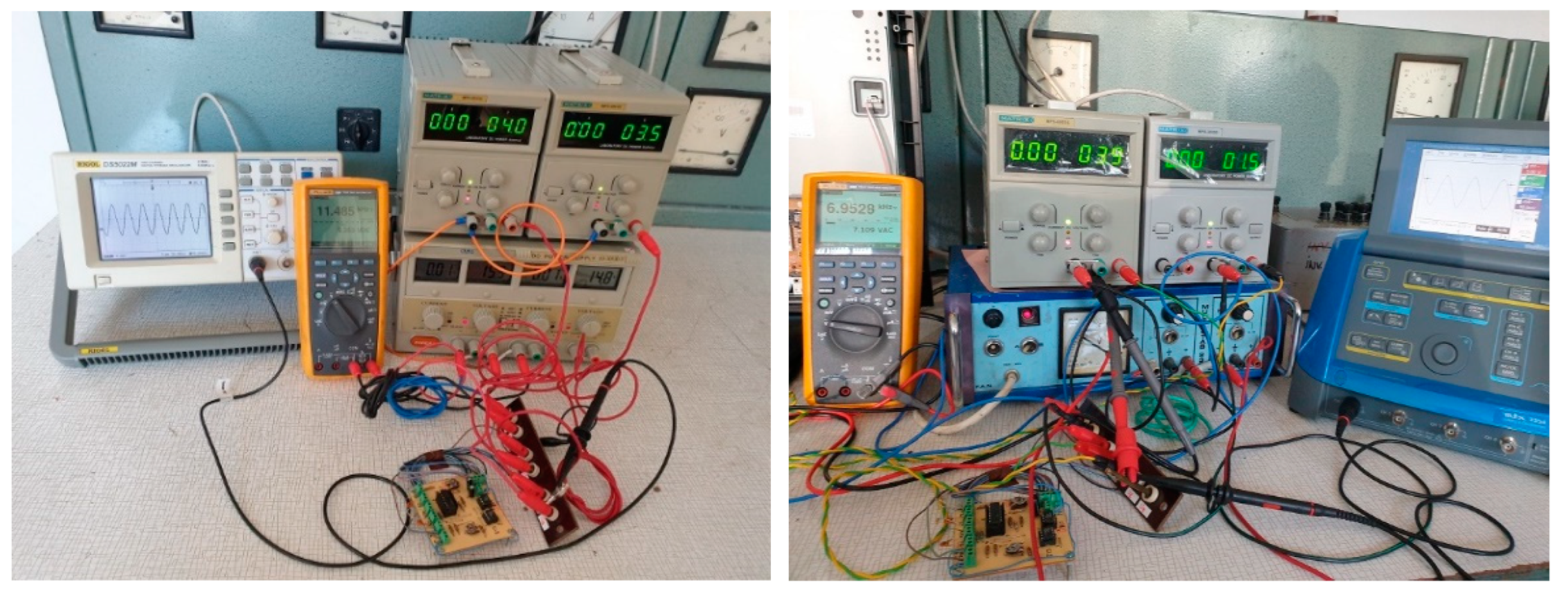
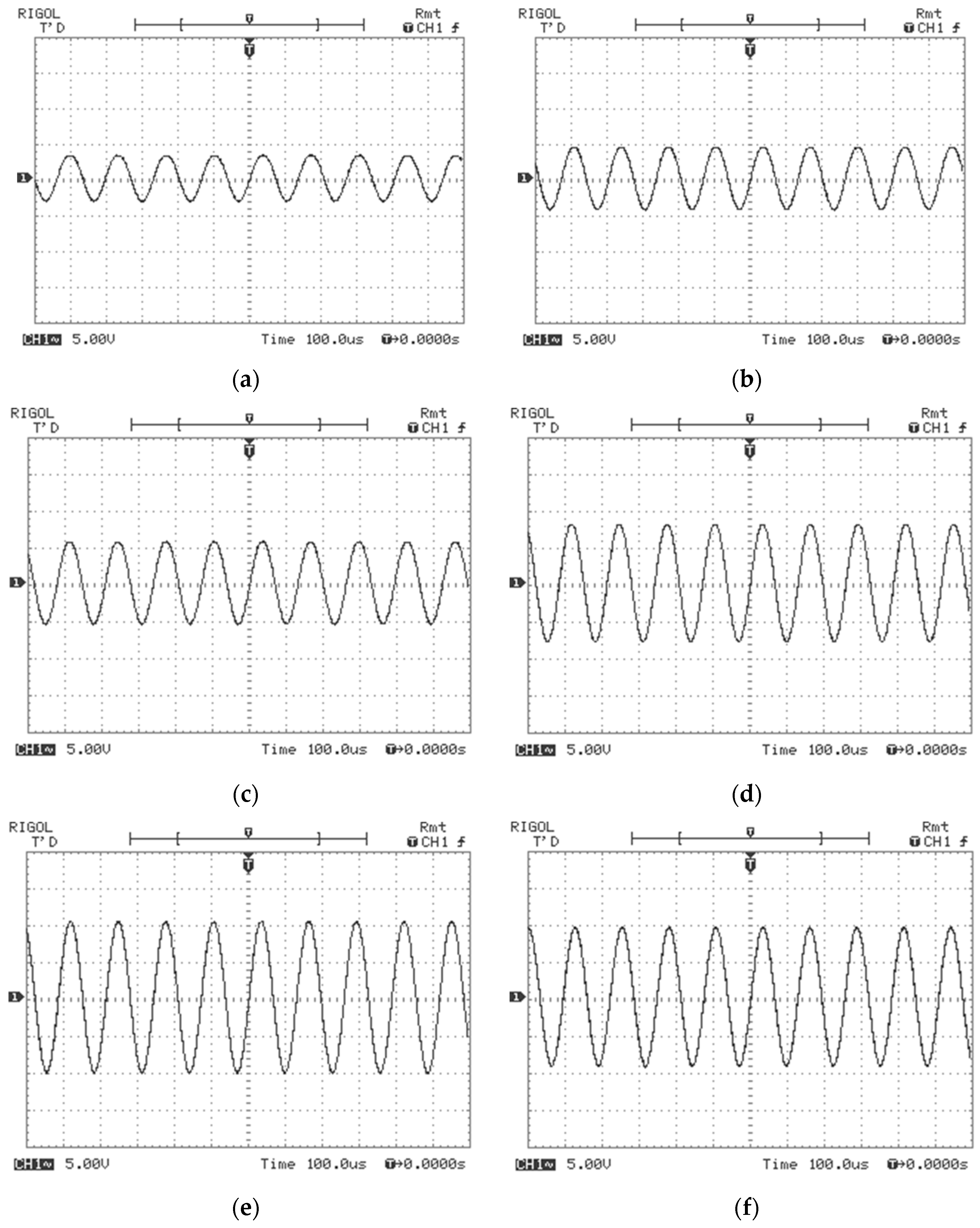
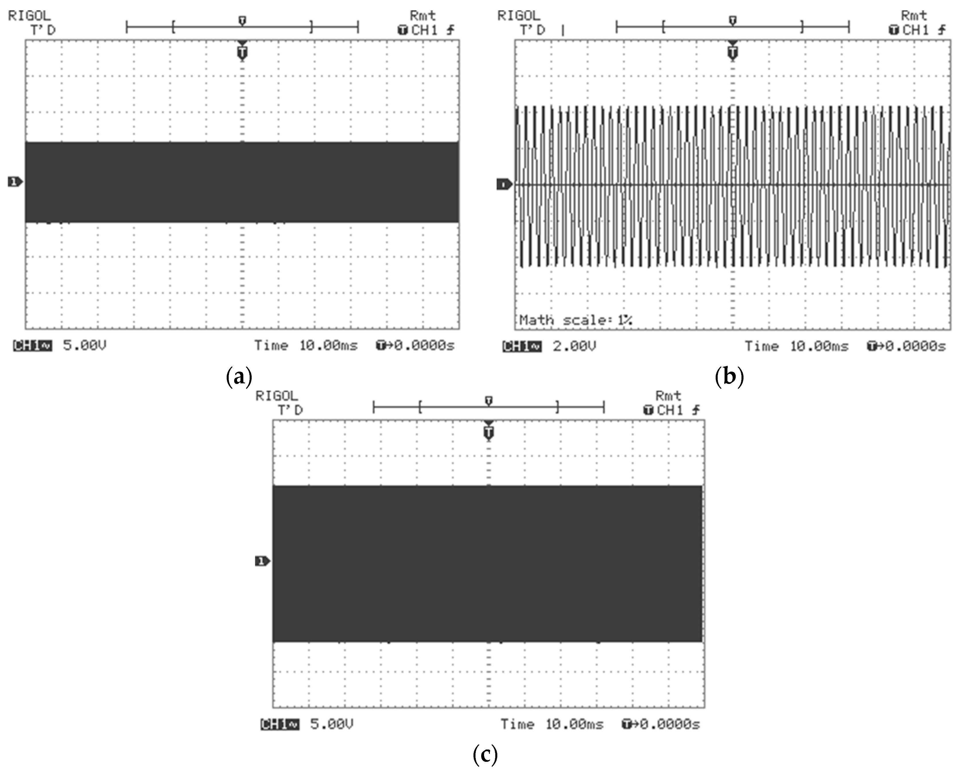
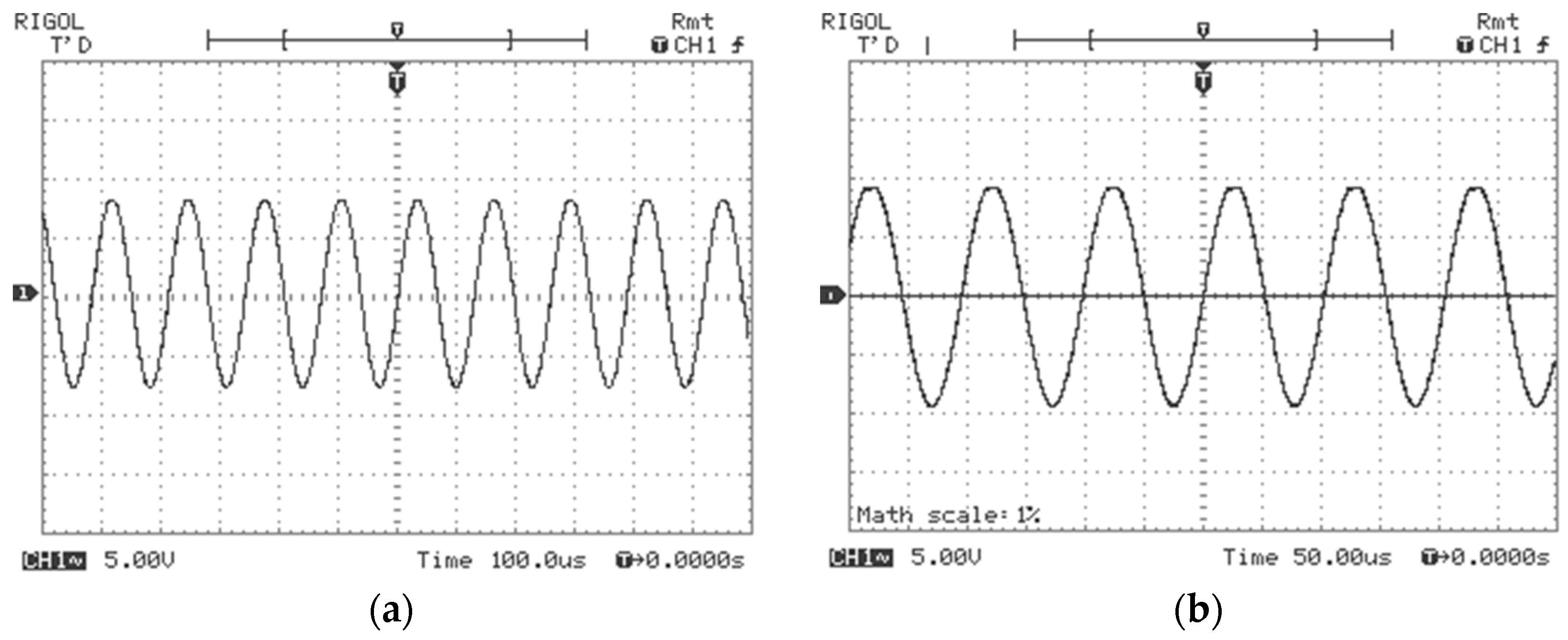
4. Experiments with Discussions

In reality, due to the limitations in the operation of electronic circuits (proportionality coefficients, multiplication coefficients, integration constants), a sinusoidal signal is obtained at the output starting from Equation (13), by the practical implementation with electronic circuits from Figure 7. Simultaneously, it has been discovered that when the u_i grows, the output signal’s amplitude u_e drops. As a result, the block diagram in Figure 7, which has seven functional blocks, is employed for the circuit’s practical realization for proper operation. There are two voltage inputs (u_i and u_f) to the sinusoidal oscillator with changeable frequency and amplitude signal. The circuits employed are two multiplication circuits, two adding circuits, a non-inverting amplifier, and two integration circuits.

The circuit in Figure 7 was used to create a sinusoidal oscillator with changeable frequency and amplitude. Two multiplier circuits (M1, (1) and M2, (2)), two adding circuits (S1, (3) and S2, (4)), a non-inverting amplifier (A1, (5)), and two integration circuits (I1, (6) and I2, (7)) make up the oscillator. The adding, amplification, and integration circuits were constructed with linear circuits (operational amplifiers), while the multiplication circuits were made with specific multiplication circuits (maximum input signals of ±10 V). The sinusoidal oscillator was created using three integrated circuits (two multipliers and one circuit with four operational amplifiers). The sinusoidal oscillator’s variable frequency and amplitude supply was kept at ±15 V for the studies. Resistances of the order of kΩ to tens of kΩ are utilized in the practical execution of the oscillator (R₁ = R₂ = R₃ = R₄; R₅ = R₆ = R₇; R₈ = R₉; R₁₂ = R₁₄; R₁₁ = R₁₃), and capacitors C₁ and C₂ are of the order of hundreds of pF.

The practical implementation was made with two analogue-integrated multiplication circuits AD633N and one linear-integrated circuit TL084 (Figure 8). The meaning of the blocks (seven pieces) in Figure 8 is the same as the meaning of the blocks in Figure 7 (e.g., (1) is a multiplication circuit, etc.).

The electronic assembly has only three integrated circuits (AD 633 JN, 2 pcs., €1.82/pc.; TL 084, €0.85/pc.), 15 resistors (€0.12/pc.), two capacitors (€0.2/pc.), connectors, printed circuit board, and wiring (approx. €0.8/pc.). The approximate price of the analogue computation converter is €7.49.

Aspects from the experiments with the sinusoidal oscillator with variable frequency and amplitude are presented in Figure 9.

The functioning restrictions of the oscillator were discovered, as expected: the constant voltages at the input cannot exceed 10 V (mandated by the multipliers’ input); the sinusoidal signal from the output can only be created over a fixed value of u_f (over 2.3 V); no sinusoidal signal is generated at the output of the oscillator at values not suitable for the integrating circuits (I1 and I2: R₁₁, C₁, R₁₃, C₂); signals that are too large (8 ÷ 10 V) for u_i to cause a non-linear change in the amplitude of the output signal u_e or for u_f to cause distortion of the output signal u_e, given that the frequency of the signal changes linearly.

For normal operation, the output signal’s waveforms (Figure 10, Figure 11 and Figure 12) were measured with a Rigol DS5022M digital oscilloscope (two channels, 25 MHz, 500 MSa/s).

The sinusoidal signal from the output of the sinusoidal oscillator in the settings where adjusting u_i (up to 7 V) results in a linear change in the signal amplitude is shown in the first set of experiments in Figure 10 and Figure 11 (for u_i greater than 7 V, the modification is slightly non-linear). The output signal’s frequency was kept constant (within a tolerable range of 1.5%).

Tests were conducted (for several input voltages) for various time periods in the second set of experiments (Figure 12) in order to determine the sinusoidal oscillator’s stable operation (maintaining the constant amplitude of the output signal). Experiments were carried out for a long period of time (up to 24 h), and the sinusoidal oscillator was discovered to have a non-damped sinusoidal mode of operation. For constant u_i and u_f, the output signal u_e maintains its sinusoidal shape and amplitude throughout time.

The frequency (f_e) and RMS value (u_e) were measured (Figure 13 and Figure 14) with a Fluke 289 digital multimeter (100 kHz frequency band). As can be seen from Figure 13, the converter works for a range of u_f; the output signal is not generated for values that are too small and for values that are limited by the supply voltage of the integrated circuits (Figure 8). In the same way, it was found for the modification of u_i (Figure 14): for values that are too small, the amplitude of the output signal does not change, and for values that are too high, the signal is distorted (deviates from the sinusoidal form). The sinusoidal signal from the output is given for when changing u_f from 2.3 V to 7 V, when the frequency of the output signal f_e changes linearly, and when u_i is constant. The output signal was not distorted and had a steady amplitude (within a reasonable range of ±1.5%).

The output signal of a converter with real components and numerous constraints (nonlinearities, input signal limitations, etc.) does not create a sinusoidal signal under any operating settings. If the DC voltage u_f is too low (less than 2.3 V), the signal from the converter’s output is shown in Figure 15. The output signal has a low amplitude and is unsteady. The output signal’s waveforms from Figure 15, Figure 16 and Figure 17 were measured with a Rigol DS5022M digital oscilloscope.

The signals for the oscillator’s output increase in the direct voltage u_f above the threshold voltage (2.3 V) and reduction in the voltage u_f below the threshold voltage are shown in Figure 16. The time it takes for the signal to stabilize is really brief. A time-stable, non-damped, sinusoidal signal is created at the output as long as u_f ≥ 2.3 V. When the DC voltage at the converter’s output is lower than 2.3 V, no steady signal is produced (the converter does not work properly). The output signal changes frequency proportionally as the input DC voltage u_f rises above 7 V, but it deforms; positive alternating is distorted (Figure 17).

5. Applications of the Analogue Computation Converter Used with Sensors

5.1. Remote Transmission of a Measured Quantity via Electrical Wires

In industrial applications, in many cases, the measuring device or the process control equipment is located at a distance of tens or even hundreds of metres from the place where the measuring sensors are mounted. Some of the measuring sensors that can measure different non-electric quantities (liquid level, pressure, temperature, flow rate, etc.) have a continuous voltage output (e.g., in the 0–10 V range), proportional to the measured quantity. The connection between the transducer and the indicating device or the control equipment is made through an electric line with two conductors, each having a resistance R_l, through which a DC current I flows (which depends on the resistance of the connecting conductors and the input impedance of the measuring device or the control equipment), on which there will be a voltage drop ΔU_l which is determined by the following formula:

$${\mathsf{\Delta }\mathrm{U}}_l=2·R_l·I$$

(16)

$${\mathsf{\Delta }\mathrm{U}}_l={\displaystyle \frac{8·\rho ·l}{\pi ·d^2}}·I$$

(17)

where ρ, l, and d are line parameters (conductor resistivity, line length, and conductor diameter). The higher the current and the length of the conductors, the higher the voltage drop will be. The loss in strength will determine a source of error in the transmission of information at a distance (the signal measured at the end of the electrical connection line is lower than the signal transmitted at the output of the transducer). The DC voltage is strongly disturbed by the electromagnetic noises in the industrial environment. For this reason, for the transmission of information at a distance through electrical wires, it is safer to transmit the information in the form of a sinusoidal signal, the frequency being more difficult to disturb in the industrial environment.

As an example, the remote transmission of the most measured non-electric quantity in the industry was chosen: temperature. Different physical effects determined by the temperature variation are used to measure the temperature. The most important of these are the variation of electrical resistance; the electromotive voltage at the junction of two metals; expansion of solids, liquids, or gases; intensity of emitted radiation; and so on. The temperature range can be higher or lower and depends on the specifics of industrial, scientific, etc. applications. Measurement over a wide temperature range cannot be covered by any of the known types of temperature sensors. Other important parameters are measurement precision, dimensions, sensitivity, stability, and response time. An analysis was made for three types of sensors (common in industry) for temperature measurement: thermistors, thermoresistances, and thermocouples.

Next, for the converter in Figure 8, a constant voltage (5 V) was kept at the u_i input in order not to change the peak-to-peak amplitude of the output sinusoidal signal, and at the u_f input, the signal coming from temperature measurement (through sensors, voltage dividers or other converters). The voltage dividers and converters that make the conversion to DC voltage, as well as the converter in Figure 8, are connected near the temperature sensor, so that after the analogue converter, a signal of a certain frequency proportional to the temperature is transmitted through the electrical line.

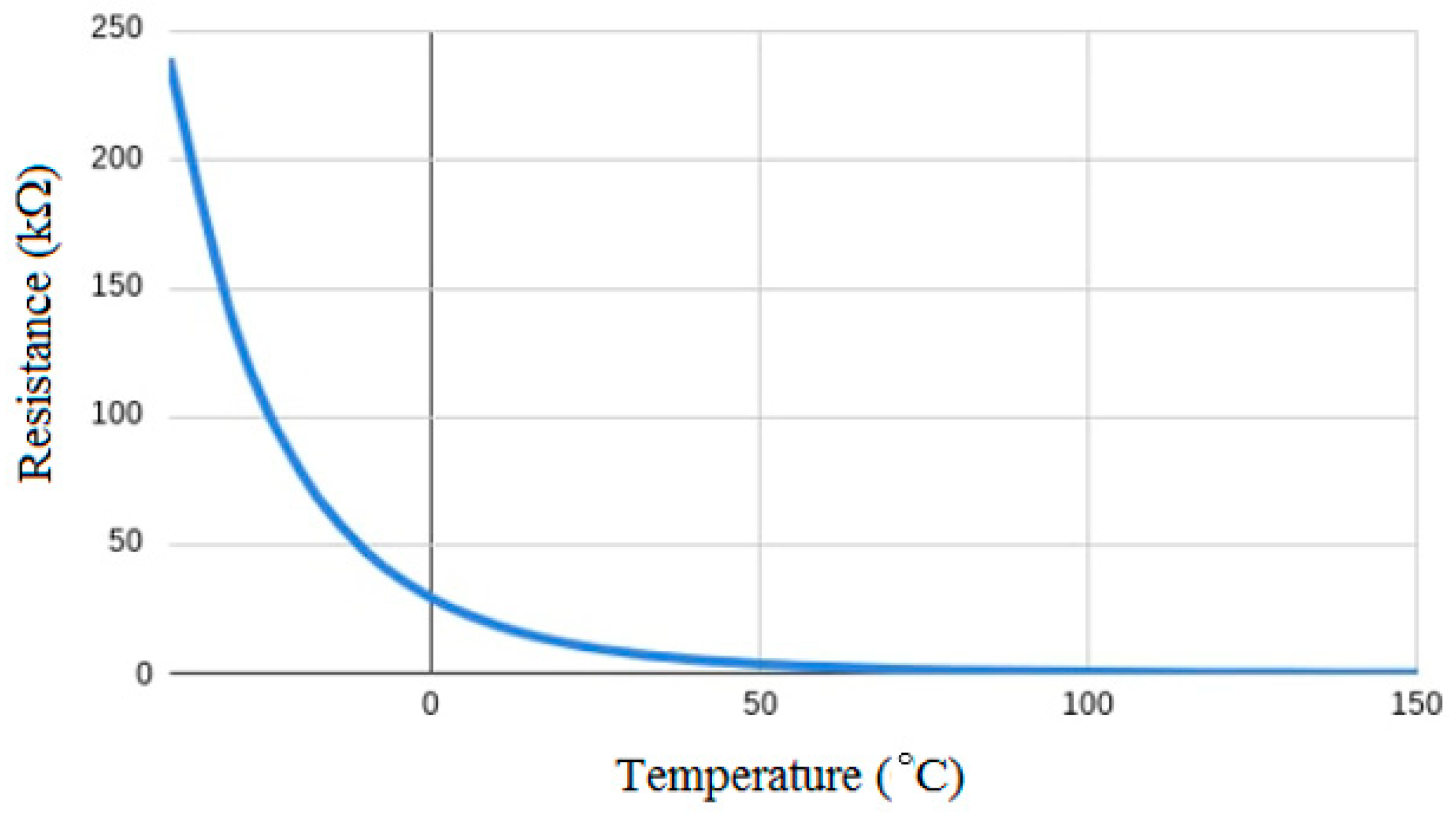
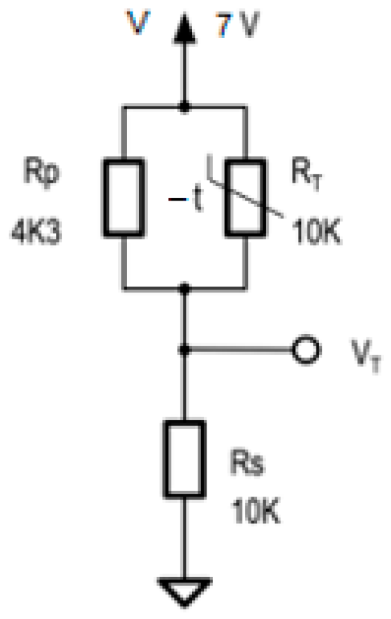
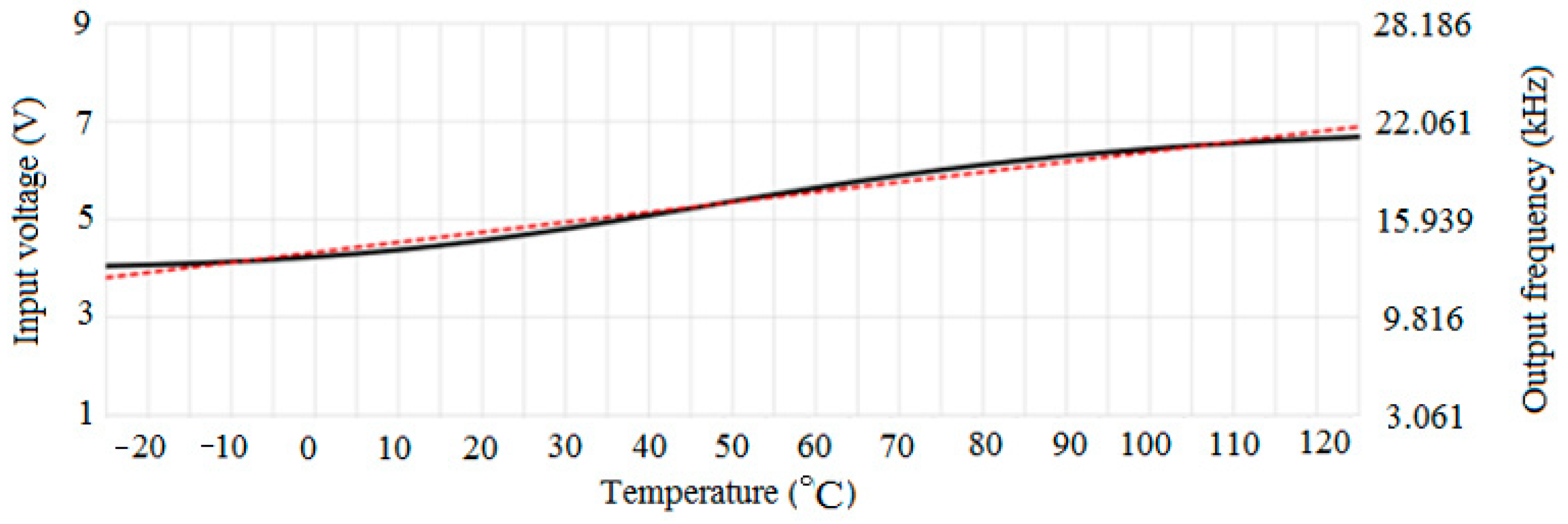
5.2. Temperature Measured with Thermistors

Thermistors are of two constructive types: with a negative characteristic (NTC) and with a positive characteristic (PTC), both types having a non-linear characteristic. The NTC thermistor used in the experiments is 10 kΩ, at 25 °C, and has the resistance temperature characteristic shown in Figure 18.

NTC thermistors are resistors with a negative temperature coefficient, the resistance decreases with increasing temperature. They are mainly used as resistive temperature sensors and current limiting devices. The temperature sensitivity coefficient is about five times that of silicon temperature sensors and about ten times that of resistance temperature sensors. NTC thermistors are typically used in a range from −55 to +200 °C. The non-linearity of the relationship between resistance and temperature exhibited by NTC thermistors has again presented a great challenge when using analogue circuits to accurately measure temperature. However, the rapid development of digital circuits has solved this problem, allowing accurate values to be calculated by interpolating look-up tables or solving equations approximating a typical NTC curve [42].

The equation gives satisfactory results, having an accuracy of ±1 °C in the range from 0 to +100 °C. It is dependent on a single material constant β which can be obtained by measurements. The equation can be written as follows:

$$R\left(T\right)=R\left(T_0\right)·e^{\beta ·\left({\displaystyle \frac{1}{T}}-{\displaystyle \frac{1}{T_0}}\right)}$$

(18)

where R(T) is the resistance at temperature T in Kelvin, and R(T₀) is the resistance of a reference point at temperature T₀. This Equation (18) requires a two-point calibration and is usually not more accurate than ±5 °C over the entire useful range of the NTC thermistor.

The best-known approximation to date is the Steinhart–Hart formula:

$${\displaystyle \frac{1}{T}}=A+B·ln\left(R\right)+C·{\left(ln\left(R\right)\right)}^3$$

(19)

where R is the resistance at temperature T (in Kelvin), and A, B, and C are coefficients derived from experimental measurements. The Steinhart–Hart formula is typically accurate to about ±0.15 °C over the range −50 to +150 °C, which is sufficient for most applications. If higher accuracy is required, the temperature range must be reduced, and an accuracy better than ±0.01 °C is possible in the range from 0 to +100 °C.

In practice, one can convert the thermistor resistance to a voltage using a voltage divider, as shown in Figure 19. By placing the NTC thermistor in the upper part of the divider, a voltage is obtained that increases with temperature, as shown in Figure 20. A 10 kΩ NTC thermistor at 25 °C was used in series with a 10 kΩ series resistance, the divider being fed to a 10 V source. Figure 20 shows that the output voltage has an S-shaped profile (solid line) around the line of best fit (dashed line).

If the divider in Figure 19 is supplied with voltage V (e.g., 10 V), then at the output of the divider, the voltage is obtained as follows:

$$V_T={\displaystyle \frac{R_S}{R_S+R_T}}·V$$

(20)

In Figure 20, the solid curve shows the output of the voltage divider, and the dotted curve is the line of best fit. The output voltage follows an S-shaped curve with a significant deviation from the ideal linear voltage–temperature relationship. At medium temperature values (about 45 °C), the error is particularly large.

If the output of the voltage divider in Figure 19 is connected to the input u_f of the converter in Figure 8, then a signal of a certain frequency is obtained at the output of the converter (Figure 20, right). As well as the voltage at the output of the resistive divider (Figure 19) and the frequency at the output of the analogue converter (Figure 8) that had a non-linear evolution depending on the measured temperature (solid line, Figure 20). If the real temperature is to be known, this curve must be linearized, through successive linearizations (as many linearizations as possible, on as few intervals as possible).

As stated, the analogue converter in Figure 8 can produce a sine–wave signal at the output if u_f (input voltage Figure 20) changes between 2.3 and 7 V. From Figure 20, it can be seen that the analogue converter in Figure 8 can be used to transmit sinusoidal signals proportional to the temperatures between −5 and 40 °C.

The linearity of voltage versus temperature can be improved by adding a resistor in parallel with the NTC thermistor, as shown in Figure 21.

If the divider in Figure 21 is supplied with voltage V, then, at the output of the divider, the voltage is obtained as follows:

$$V_T={\displaystyle \frac{R_S}{R_S+\frac{R_T·R_P}{R_T+R_P}}}·V$$

(21)

Adding a resistor in parallel with the thermistor improves the voltage–temperature linearity, if the values are chosen appropriately (Figure 21). The R_p value (4.3 kΩ) was chosen to be similar to the thermistor resistance at 45 °C to maximize linearity over the temperature range. It can be seen that the voltage curve (solid line) much better approximates the line of best linear fit (dashed line), the measurement errors being smaller than in the previous case.

Adding a parallel resistor improves linearity significantly. This improvement comes at the expense of the signal’s dynamic range, which is now only about 3 V compared to 9 V. Dynamic range and linearity can be optimized by carefully adjusting series and parallel resistors. Better results are also obtained if a narrow temperature range is desired.

If the output of the divider in Figure 22 is connected to the uf input of the converter (Figure 8), at its output, a frequency is obtained that changes almost proportionally to the measured temperature.

By using the divider in Figure 21, the temperature can be measured for a much wider range, between −20 and 120 °C, and the measured temperature can be transmitted in the form of a sinusoidal signal using the analogue converter in Figure 8.

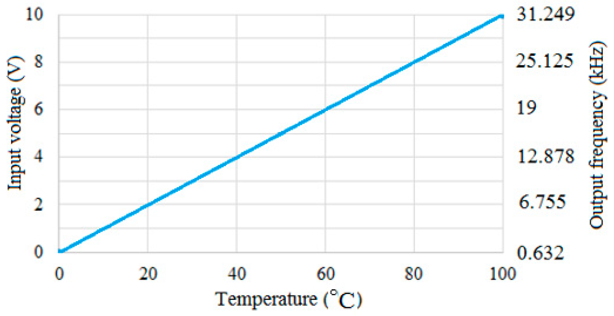
5.3. Temperature Measured with Resistance Temperature Detector

An RTD (Resistance Temperature Detector) is a temperature sensor whose resistance changes as the temperature changes. The resistance increases as the temperature of the transducer increases. The resistance relationship depending on the temperature is known and is repeatable over time. A thermistor is a passive device and does not produce an analogue output (voltage or current) on its own. External electronics are used to measure the resistance of the transducer by passing a small electric current through it to generate a voltage. Typically, a current between 1 mA (or even less) and a maximum of 5 mA (without the risk of self-heating) is used.

Typically, resistance thermometers are constructed of platinum, nickel, or copper. The most common thermoresistance in the industry is Pt 100 (Platinum transducer, 100 Ω at 0 °C). For the Pt 100 thermoresistance, the following formulas can be used [43]:

$$R_t=R_0·\left(1+a·t+b·t^2+c·t^3\left(t-100\right)\right)$$

(22)

for t < 0 °C, and:

$$R_t=R_0·\left(1+a·t+b·t^2\right)$$

(23)

for t > 0 °C, where R_t is the resistance of the thermistor at temperature t; R₀ (100 Ω) is the resistance of the thermistor at the temperature of 0 °C; and a, b, and c are coefficients given in the catalogues.

For positive temperatures, for simplification can be use the following:

$$R_t=R_0·\left(1+a·t\right)$$

(24)

where a = 385 mΩ/°C, because b is very small.

Usually, to obtain a direct voltage proportional to the measured temperature, converters specially built for Pt100 can be used, with output 0–10 V DC (Schneider Electric, RMPT30BD type, France of Rueil-Malmaison, Ile de France). The converter has the following characteristics: it is used with the Pt 100 thermoresistance; powered at 24 V DC; measuring range 0–100 °C; output voltage 0–10 V DC; accuracy 0.2%; sensitivity 100 mV/°C. Figure 23 shows the characteristic of the RMPT30BD resistance–temperature converter.

If the output of the DC voltage–temperature converter is connected to the u_f input of the converter (Figure 8), at its output, a frequency is obtained that changes proportionally to the measured temperature (Figure 23, right). The temperature that can be measured is between 23 and 70 °C (for which a sinusoidal signal is obtained).

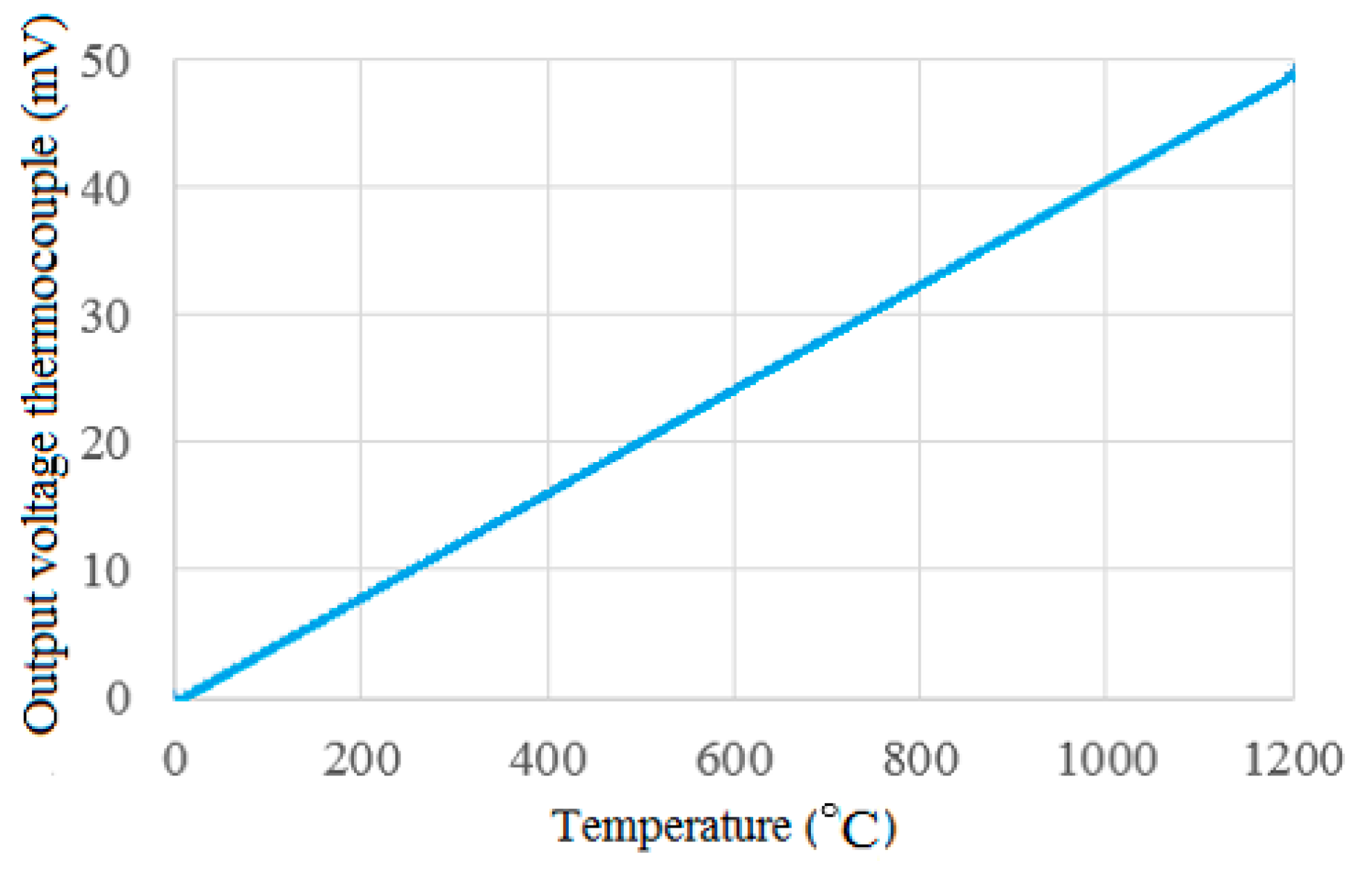
5.4. Temperature Measured with Thermocouples

Thermocouples are the most widespread temperature transducers in the industry, for a very wide range of temperatures and a variety of measurement conditions. They are based on the thermoelectric effect: the appearance of an electromotive voltage in a circuit made of two different metals depending on the difference between the temperatures of the two junctions. The usual thermocouple consists of two wires of different metals or alloys (there are many combinations), welded together to form a measuring junction (or hot junction) and a reference junction (or cold junction). The measured temperature is actually the temperature difference between the two junctions. To measure absolute temperatures, it is necessary that the reference junction be maintained at a constant temperature. For different thermocouples, there are temperature ranges where the output voltage change (of the order of mV or tens of mV) changes linearly with temperature [44]. A converter often used in the industry to which various types of thermocouples can be connected (type B, E, J, K, L, N, R, S, T, U, C) is the LKM 282 (Electrotherm Digital Transducer, Geraberg, Germany). The configuration (choosing the type of thermocouple) is conducted through a programmer (via mini USB), and at the output, a continuous voltage between 0 and 10 V, DC is obtained; the supply is made from 8 to 35 V DC; smoothness error 0.3 K; measurement error 0.2%; response time 0.5 s. The thermoelectric voltages of the transducers are converted temperature-linearly into the output signal ranging from 0 to 10 V.

One of the most common thermocouples, type K (cromel–alumel), was chosen. Figure 24 shows the voltage–temperature characteristic for the K-type thermocouple. The measurement range is from 0 to 1200 °C.

From Figure 24 and Figure 25, it can be seen that when the two converters (LKM 282 and the converter from Figure 8) are connected, a signal with a frequency directly proportional to the temperature measured by the thermocouple is obtained at the output. The temperature that can be measured is between 300 and 900 °C (for which a sinusoidal signal is obtained).

6. Conclusions

Modelling, simulation, and experimentation of an analogue computation converter with variable frequency and amplitude yielded the following results:

–

An analogue computer was developed using the nonhomogeneous second-order linear ordinary differential equation to adjust the frequency and amplitude of the sinusoidal signal at the output using two DC voltages;

–

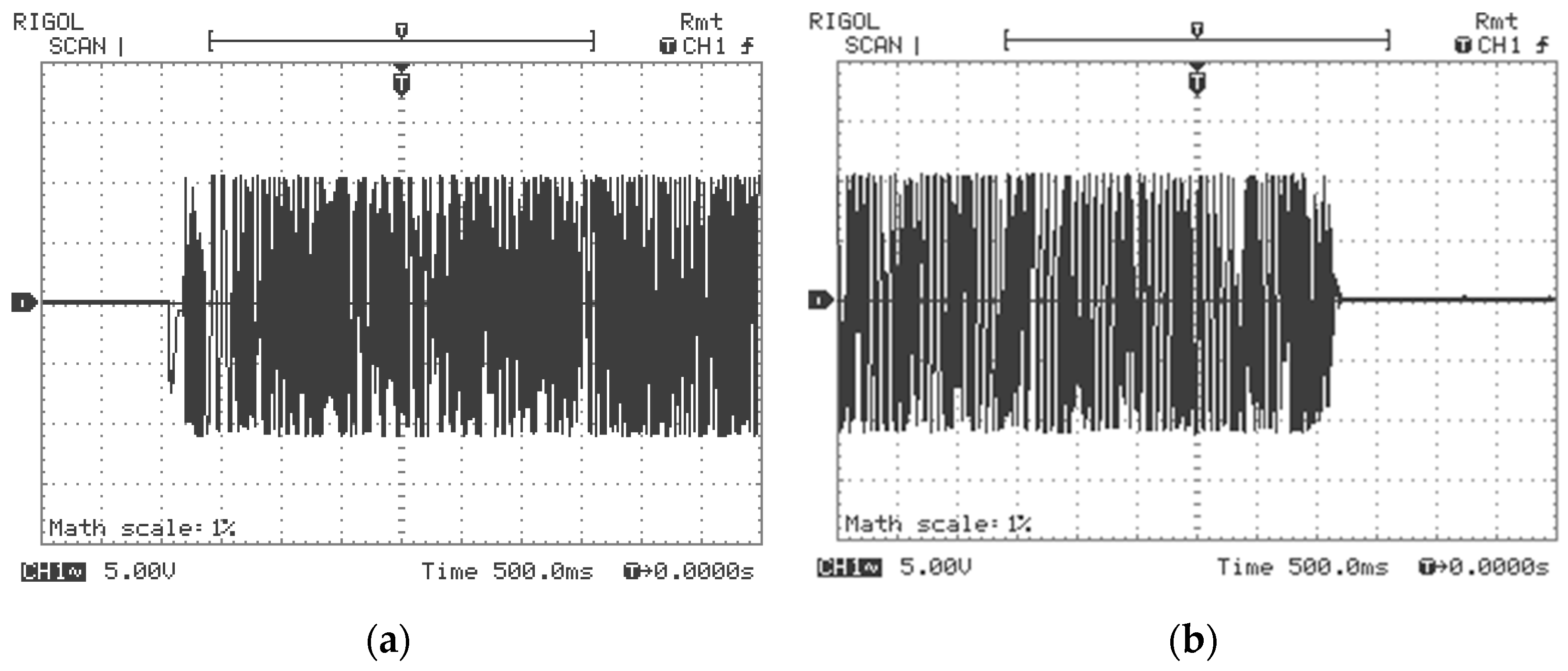
The output signal for u_i and u_f is sinusoidal and stable over time over a variety of DC voltages (non-damped operation mode);

–

The analogue converter has a straightforward design with two DC voltage inputs and one (sinusoidal voltage) output;

–

The response time is relatively short because the sinusoidal converter is only realised with analogue components;

–

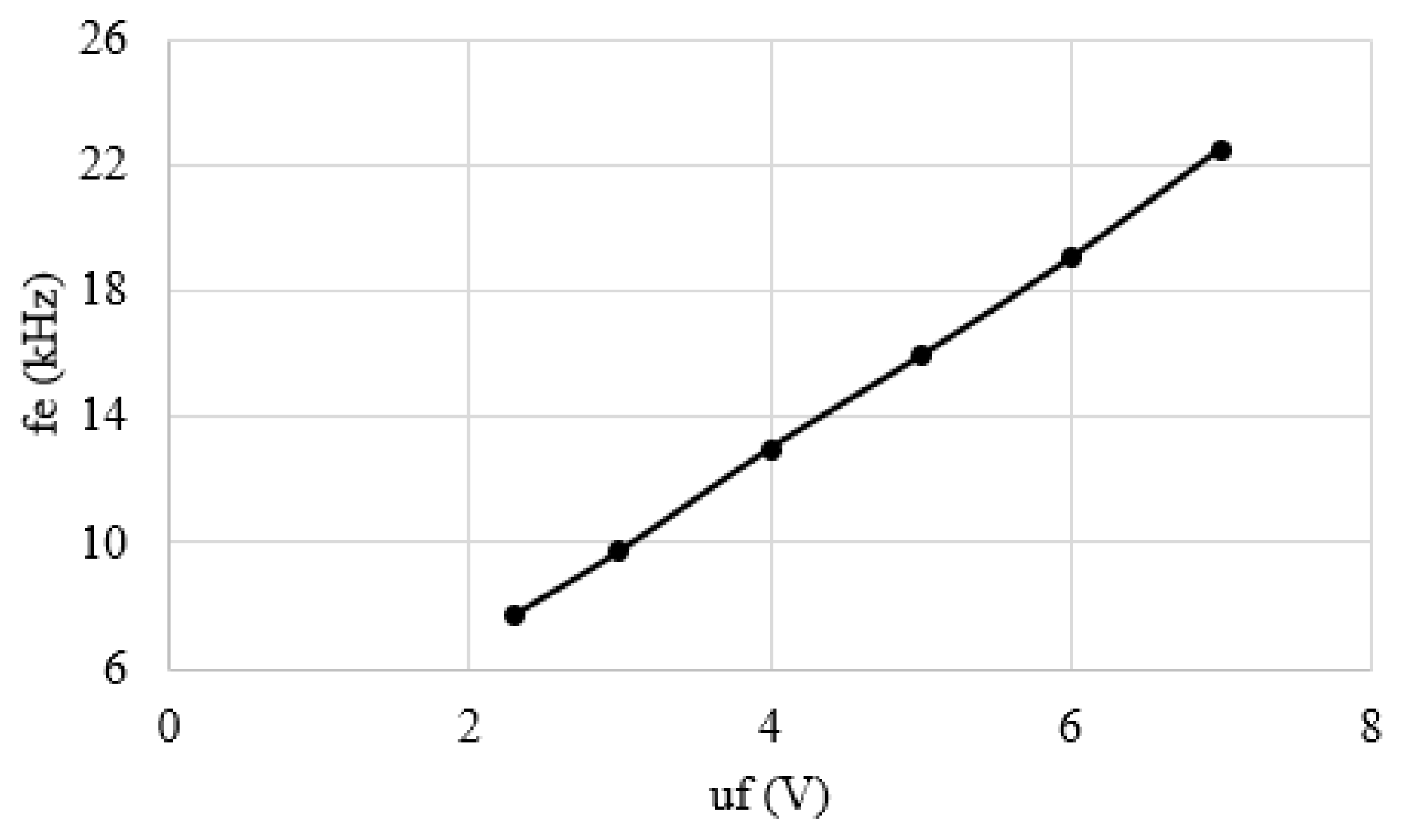
The output signal has a frequency in the kHz range, and the operating range might be in the tens of kHz range;

–

The u_f input of the sinusoidal converter can be used on analogue sensors that have a DC voltage at the output to convert the voltage into a sinusoidal signal.

The following (for transducer applications) will be the focus of future investigations using the analogue computation converter with variable frequency and amplitude:

–

The precise determination of the R-C component limit values for the I1 and I2 integrated circuits, for which the sinusoidal signal at the oscillator’s output has a linear dependence (amplitude and frequency) on the DC voltages at the input;

–

Connecting resistive (for linear, angular displacements, and so on) and capacitive transducers (liquid-level gauges, pressure metres, accelerometers, precision positioners, and so on) to integration circuits to convert the signals into a sinusoidal output signal proportional to the input size of the sensors;

–

Studies on signals with noise at the input of the converter to study the influence on the output of the converter.

7. Patents

The article is based on the concept of patent No. 130458, “Linear voltage converter—variable frequency sinusoidal signal“, from 30 May 2022 at the Office of State for Inventions and Trademarks in Bucharest, Romania.

References

1. Abuelma’atti, M.T.; Al-Ali, A.K.; Buhalim, S.S.; Ahmed, S.T. Digitally Programmable Partially Active-R Sinusoidal Oscillators. Act. Passiv. Electron. Compon. 1994, 17, 83–89. [Google Scholar] [CrossRef]
2. Adragna, C.; Gritti, G.; Raciti, A.; Rizzo, S.A.; Susinni, G. Analysis of the Input Current Distortion and Guidelines for Designing High Power Factor Quasi-Resonant Flyback LED Drivers. Energies 2020, 13, 2989. [Google Scholar] [CrossRef]
3. Baek, S.; Choi, D.; Bu, H.; Cho, Y. Analysis and Design of a Sine Wave Filter for GaN-Based Low-Voltage Variable Frequency Drives. Electronics 2020, 9, 345. [Google Scholar] [CrossRef]
4. Groner, S. Low Distortion Oscillator Design. Master’s Thesis, Zurich University of the Arts, Zurich, Switzerland, 2010; pp. 1–88. [Google Scholar]
5. Mechergui, H.; Haddouk, A. Amplitude control in sinusoidal oscillator. In Proceeding of the International Conference MS’07, Kolkata, India, 3–5 December 2007; pp. 1–7. [Google Scholar]
6. Hong, B.; Hajimiri, A. A Phasor-Based Analysis of Sinusoidal Injection Locking in LC and Ring Oscillators. IEEE Trans. Circuits Syst. I 2019, 66, 355–368. [Google Scholar] [CrossRef]
7. Linares-Barranco, B.; Rodriguez-Vázquez, A.; Sánchez-Sinencio, E.; Huertas, J.L. CMOS OTA-C High-Frequency Sinusoidal Oscillators. IEEE J. Solid State Circuits 1991, 26, 160–165. [Google Scholar] [CrossRef]
8. Osa, J.I.; Carlosena, A. MOSFET-C Sinusoidal Oscillator with Variable Frequency and Amplitude. In Proceedings of the 2000 IEEE International Symposium on Circuits and Systems (ISCAS), Geneva, Switzerland, 28–31 May 2000; pp. 1–6. [Google Scholar]
9. Jaikla, W.; Adhan, S.; Suwanjan, P.; Kumngern, M. Current/Voltage Controlled Quadrature Sinusoidal Oscillators for Phase Sensitive Detection Using Commercially Available IC. Sensors 2020, 20, 1319. [Google Scholar] [CrossRef]
10. Lepkowski, J. Designing Operational Amplifier Oscillator Circuits for Sensor Applications; AN 866 DS00866A; Microchip Tehnology Inc.: Chandler, AZ, USA, 2003; pp. 1–16. [Google Scholar]
11. Hybrid Oscillator and Demodulator LDT Modules; Solartron Metrology: Bognor Regis, UK, 2021.
12. Oscilloscope Fundamentals; Tektronix: Singapore, 2022.
13. Williams, J. Instrumentation Applications for a Monolithic Oscillator. A Clock for All Reasons; Application Note 93; Linear Technology Corporation: Milpitas, CA, USA, 2003; pp. 1–20. [Google Scholar]
14. Oukaira, A.; Mellal, I.; Ettahri, O.; Tabaa, M.; Lakhssassi, A. Simulation amd FPGA Implementation of a Ring Oscillator Sensor for Complex System Design, Special Issue on Advancement in Engineering Technology. Adv. Sci. Technol. Eng. Syst. J. 2018, 3, 317–321. [Google Scholar] [CrossRef]
15. Oscillator Design Guide for STM8AF/AL/S, STM32 MCUs and MPUs; AN 2867 Application Note; STMicroelectronics: Geneva, Switzerland, 2020.
16. Serra, F.M.; Fernándezm, L.M.; Montoya, O.D.; Gil-González, W.; Hernández, J.C. Nonlinear Voltage Control for Three-Phase DC-AC Converters in Hybrid Systems: An Application of the PI-PBC Method. Electronics 2020, 9, 847. [Google Scholar] [CrossRef]
17. Sagbas, M.; Ayten, U.E.; Herencsar, N.; Minaei, S. Current and Voltage Mode Multiphase Sinusoidal Oscillators Using CBTAs. RadioEngineering 2013, 22, 24–33. [Google Scholar]
18. Cheng, J.; Chen, D.; Chen, G. Modeling and Compensation for Dead-Time Effect in High Power IGBT/IGCT Converters with SHE-PWM Modulation. Energies 2020, 13, 4348. [Google Scholar] [CrossRef]
19. Fiore, J.M. Operational Amplifiers & Linear Integrated Circuits: Theory and Application; Creative Commons: Mountain View, CA, USA, 2020; pp. 1–589. [Google Scholar]
20. Gasulla, M.; Li, X.; Meijer, G.C.M. The Noise Performance of a High-Speed Capacitive-Sensor Interface Based on a Relaxation Oscillator and a Fast Counter. IEEE Trans. Instrum. Meas. 2005, 54, 1934–1940. [Google Scholar] [CrossRef]
21. Mancini, R.; Palmer, R. Sine-Wave Oscillator; Application Report SLOA060; Texas Instruments: Dallas, TX, USA, 2001; pp. 1–21. [Google Scholar]
22. Pandiev, I.M.; Todorov, T.G.; Yakimov, P.I.; Doychev, D.D. A Practical Approach to Design and Analysis Sinusoidal Oscillators. Annu. J. Electron. 2009, 92–95. [Google Scholar]
23. Stave, N.J. Analysis of BJT Colpitts Oscillators—Empirical and Mathematical Methods for Predicting Behavior. Master’s Thesis, Marquette University, Milwaukee, WI, USA, 2009; pp. 1–151. [Google Scholar]
24. Rivera, M.; Rojas, S.; Restrepo, C.; Muñoz, J.; Baier, C.; Wheeler, P. Control Techniques for a Single-Phase Matrix Converter. Energies 2020, 13, 6337. [Google Scholar] [CrossRef]
25. Chang, E.C. High-Performance Pure Sine Wave Inverter with Robust Intelligent Sliding Mode Maximum Power Point Tracking for Photovoltaic Applications. Micromachines 2020, 11, 585. [Google Scholar] [CrossRef]
26. Vasan, B.K. Waveform Generation in Phase Shift Oscillators Using Harmonic Programming Techniques. Ph.D. Thesis, Iowa State University, Ames, IA, USA, 2013; pp. 1–151. [Google Scholar]
27. Sotner, R.; Jerabek, J.; Herencsar, N.; Horng, J.W.; Vrba, K.; Dostal, T. Simple Oscillator with Enlarged Tunability Range Based on ECCII and VGA Utilizing Commercially Available Analog Multiplier. Meas. Sci. Rev. 2016, 16, 35–41. [Google Scholar] [CrossRef]
28. Lahiri, A. New Canonic Active RC Sinusoidal Oscillator Circuits Using Second-Generation Current Conveyors with Application as a Wide-Frequency Digitally Controlled Sinusoid Generator. Act. Passiv. Electron. Compon. 2011, 2011, 274394. [Google Scholar] [CrossRef]
29. Mittal, N.; Charan, P.; Majeed, F. A Novel Tunable High Frequency Sinusoidal Oscillator Based on the Second Generation Current Controlled Conveyor. Int. J. Sci. Res. Publ. 2013, 3, 2250–3153. [Google Scholar]
30. Khandi, M.R. Modeling and Estimation of Phase Noise in Oscillators with Colored Noise Sources. Ph.D. Thesis, Chalmers University of Technology, Göteborg, Sweden, 2013. Technical Report No. R019. pp. 1–90. [Google Scholar]
31. Razavi, B. A Study of Phase Noise in CMOS Oscillators. IEEE J. Solid State Circuits 1996, 31, 331–343. [Google Scholar] [CrossRef]
32. Yan, J. A Low Total Harmonic Distortion Sinusoidal Oscillator Based on Digital Harmonic Cancellation Technique. Master’s Thesis, Texas A&M University, College Station, TX, USA, 2012; pp. 1–129. [Google Scholar]
33. Yamaguchi, T.; Ueno, A. Capacitive-Coupling Impedance Spectroscopy Using a Non-Sinusoidal Oscillator and Discrete-Time Fourier Transform: An Introductory Study. Sensors 2020, 20, 6392. [Google Scholar] [CrossRef]
34. Odame, K.M.; Hasler, P. Theory and Design of OTA-C Oscillators with Native Amplitude Limiting. IEEE Trans. Circuits Syst. I Regul. Pap. 2009, 56, 40–50. [Google Scholar] [CrossRef]
35. Kolářová, E.; Brančík, L. Application of Stochastic Differential Equations in Second-Order Electrical Circuits Analysis. Przegląd Elektrotechniczny 2012, 88, 103–107. [Google Scholar]
36. Maoil´eidigh, D.Ó.; Hudspeth, A.J. Sinusoidal-Signal Detection by Active, Noisy Oscillators on The Brink of Self-Oscillation. Phys. D Nonlinear Phenom. 2018, 378–379, 33–45. [Google Scholar] [CrossRef]
37. Priandana, E.R.; Noguchi, T. Pure Sinusoidal Output Single-Phase Current-Source Inverter with Minimized Switching Losses and Reduced Output Filter Size. Electronics 2019, 8, 1556. [Google Scholar] [CrossRef]
38. Sullivan, D.B.; Allan, D.W.; Howe, D.A.; Walls, W.L. Characterization of Clocks and Oscillators; National Institute of Standards and Technology: Gaithersburg, MD, USA, 1990; pp. 1–364. [Google Scholar]
39. Tindel, S. Second Order Linear Equations. Differential Equations; Purdue University: West Lafayette, IN, USA, 2019; pp. 1–115. [Google Scholar]
40. Jang, J. Transient Analysis, Chapter 5, Electrical Engineering; Chung-Ang University: Seoul, Republic of Korea, 2018; pp. 1–22. [Google Scholar]
41. Korn, G.A.; Korn, T.M. Electronic Analog and Hybrid Computers, 2nd ed.; McGraw-Hill: New York, NY, USA, 1972. [Google Scholar]
42. Potter, D. Measuring Temperature with Thermistor—A Tutorial. National Instruments, Application Note 065, 340904B-01, November 1996, 8 p. Available online: https://users.wpi.edu/~sullivan/ME3901/Laboratories/03-Temperature_Labs/Thermistor_an065.pdf (accessed on 16 June 2024).
43. Resistance Temperature Detectors (RTDs); Thermo Sensor Corporation: Garland, TX, USA, 2013.
44. Park, R.M. Thermocouple Fundamentals; Marlin Manufacturing Corporation: Cleveland, OH, USA, 2015. [Google Scholar]
Figure 1. y(t) response depending on ξ (Equation (6)).
Computation 12 00169 g001
Figure 2. Theoretical block diagram of analogue computers that fulfill the function of an analogue sinusoidal oscillator with variable frequency and amplitude.
Computation 12 00169 g002
Figure 3. Block diagram for an analogue computation converter with changeable frequency and amplitude made in Simulink/Matlab R2014.
Computation 12 00169 g003
Figure 4. Output signal when: (a) Ci = 3, Cf = 3, fe = 4.694 kHz, Vepp = 6, VeRMS = 2.127; (b) Ci = 3, Cf = 7, fe = 11.11 kHz, Vepp = 6, VeRMS =2.127; (c) Ci = 3, Cf = 11, fs = 17.094 kHz, Vepp = 6, VeRMS = 2.127; (d) Ci = 3, Cf = 15, fs = 24.57 kHz, Vepp = 6, VeRMS = 2.127 (time (s) on horizontal axis; the output signal amplitude on vertical axis).
Computation 12 00169 g004
Figure 5. Output signal when: (a) Ci = 1, Cf = 9, fs = 14.326 kHz, Vepp = 2, VeRMS = 0.709; (b) Ci = 3, Cf = 9, fs = 14.326 kHz, Vepp = 6, VeRMS =2.127; (c) Ci = 5, Cf = 9, fs = 14.326 kHz, Vepp = 10, VeRMS =3.546; (d) Ci = 7, Cf = 9, fs = 14.326 kHz, Vepp = 14, VeRMS = 4.964 (time (s) on horizontal axis; the output signal amplitude on vertical axis).
Computation 12 00169 g005
Figure 6. Output signal when: (a) Ci = 1, Cf = 9, fs = 14.326 kHz, Vepp = 2, VeRMS = 0.709; (b) Ci = 3, Cf = 9, fs = 14.326 kHz, Vepp = 6, VeRMS = 2.127; (c) Ci = 5, Cf = 9, fs = 14.326 kHz, Vepp = 10, VeRMS = 3.546; (d) Ci = 7, Cf = 9, fs = 14.326 kHz, Vepp = 14, VeRMS = 4.964 (time (s) on horizontal axis; the output signal amplitude on vertical axis).
Computation 12 00169 g006
Figure 7. An electronic diagram of the analogue computation converter.
Computation 12 00169 g007
Figure 8. Practical electronic diagram of analogue computation converter.
Computation 12 00169 g008
Figure 9. Aspects of experiments with a analogue computation converter.
Computation 12 00169 g009
Figure 10. Sinusoidal output signal (constant frequency, fe = 7.73 kHz) for: (a) ui = 0 V; uf = 2.3 V; ueRMS = 2.628 V; (b) ui = 1 V; uf = 2.3 V; ueRMS = 3.706 V; (c) ui = 2 V; uf = 2.3 V; ueRMS = 3.94 V; (d) ui = 4 V; uf = 2.3 V; ueRMS = 5.616 V; (e) ui = 6 V; uf = 2.3 V; ueRMS = 7.219 V; (f) ui = 8 V; uf = 2.3 V; ueRMS = 6.652 V.
Computation 12 00169 g010
Figure 11. Output sinusoidal signal for: (a) ui = 2 V; uf = 2.3 V; fe = 7.623 kHz; ueRMS = 3.899 V; (b) ui = 0 V; uf = 3 V; fe = 9.576 kHz; ueRMS =1.0 V; (c) ui = 6 V; uf = 5 V; fe = 15.819 kHz; ueRMS = 7.471 V.
Computation 12 00169 g011
Figure 12. Sinusoidal output signal (constant amplitude, ueRMS = 5.923 V) for: (a) ui = 4 V; uf = 2.3 V; fe = 7.73 kHz; (b) ui = 4 V; uf = 3 V; fe = 9.754 kHz; (c) ui = 4 V; uf = 4 V; fe = 13.008 kHz; (d) ui = 4 V; uf = 5 V; fe = 15.921 kHz; (e) ui = 4 V; uf = 6 V; fe = 19.028 kHz.
Computation 12 00169 g012aComputation 12 00169 g012b
Figure 13. The frequency of the sinusoidal signal fe from the output as a function of uf (DC voltage) when ui (DC voltage) is constant.
Computation 12 00169 g013
Figure 14. RMS voltage of the sinusoidal output signal ueRMS as a function of the input voltage ui (DC voltage) when uf is constant (DC voltage).
Computation 12 00169 g014
Figure 15. Output signal for ui = 10 V; uf = 2.25 V; fe = 7.57 kHz; and ueRMS = 0.424 V.
Computation 12 00169 g015
Figure 16. Output signal for ui = 5 V; uf = 5 V; fe = 15.819 kHz; ueRMS = 2.515 V: (a) when the uf voltage increases above 2.3 V (threshold voltage) up to 5 V; (b) when the uf voltage drops from 5 V to below 2.3 V (threshold voltage).
Computation 12 00169 g016
Figure 17. Output signal for (a) ui = 0 V; uf = 8 V; fe = 21.098 kHz; usRMS =1.1458 V; (b) ui = 0 V; uf = 10 V; fe = 26.580 kHz; ueRMS = 1.2344 V.
Computation 12 00169 g017
Figure 18. The characteristic of the NTC thermistor with the value of 10 kΩ at 25 °C.
Computation 12 00169 g018
Figure 19. Resistive divider with NTC thermistor and resistance connected in series.
Computation 12 00169 g019
Figure 20. The voltage at the output of the divider in Figure 19 depending on the temperature (left) and the frequency at the output of the converter (Figure 8) depending on the temperature (right)—solid line; linearization of the transducer—broken line.
Computation 12 00169 g020
Figure 21. Using series and parallel resistors with the thermistor.
Computation 12 00169 g021
Figure 22. The voltage at the output of the divider in Figure 21 depending on the temperature (left) and the frequency at the output of the converter (Figure 8) depending on the temperature (right)—solid line; linearization of the transducer—broken line.
Computation 12 00169 g022
Figure 23. The characteristic of the DC voltage–temperature converter (left, RMPT30BD) and the frequency–temperature characteristic when the converter of Figure 8 (right) is also used.
Computation 12 00169 g023
Figure 24. Voltage–temperature characteristic for thermocouple type K (cromel–alumel).
Computation 12 00169 g024
Figure 25. The DC voltage–thermocouple voltage characteristic for the LKM 282 converter (left) and the frequency–thermocouple voltage characteristic for the converter in Figure 8 connected to the LKM 282 converter (right).
Computation 12 00169 g025