Abstract
Outlier detection, or anomaly detection as it is known in the machine learning community, has gained interest in recent years, and it is commonly used when the sample size is smaller than the number of variables. In 2015, an outlier detection procedure was proposed 7 for this high-dimensional setting, replacing the classic minimum covariance determinant estimator with the minimum diagonal product estimator. Computationally speaking, their method has two drawbacks: (a) it is not computationally efficient and does not scale up, and (b) it is not memory efficient and, in some cases, it is not possible to apply due to memory limits. We address the first issue via efficient code written in both R and C++, whereas for the second issue, we utilize the eigen decomposition and its properties. Experiments are conducted using simulated data to showcase the time improvement, while gene expression data are used to further examine some extra practicalities associated with the algorithm. The simulation studies yield a speed-up factor that ranges between 17 and 1800, implying a successful reduction in the estimator’s computational burden.
MSC:
6208; 62H99
1. Introduction
High-dimensional data are frequently obtained in the current era in many scientific fields, with the most prevalent field being that of bioinformatics, where the number of variables (p) far exceeds the sample size (n). For instance, gene expression datasets usually number more than 50,000 variables but only a few hundred observations. On the other hand, genome-wide association study datasets could count more than 200,000 variables. Adding to this, the rapid growth in data availability and volume necessitates not only high computing power but also efficient and scalable statistical and machine learning algorithms.
However, in general, statistical and machine learning algorithms are not robust to outliers in data. Outliers is a frequently met phenomenon that has been long and well-studied in the area of statistics. The statistical literature concerning outlier detection methods and algorithms robust to outliers is vast [1] and dates back decades. However, it must be made clear that there is a clear distinction between outlier detection and robust algorithms. The first category of algorithms detect the (possible or candidate) outlying observations in order to be removed from subsequent analyses, whereas the latter category employs algorithms that provide low weight in these values, without removing them. In the machine learning community, outlier detection is better known as anomaly detection [2], but regardless of the terminology used, the concept is the same, i.e., the detection of possibly unusual observations.
Outlier detection in the context has been extensively studied. Furthermore, outlier detection within the high-dimensional data setting () has recently gained research interest due to the fact that traditional techniques are not applicable within this frame. In [3], the authors proposed a new procedure for detecting outliers in high-dimensional data sets. The method relies on the classical minimum covariance determinant (MCD) estimator [4], but employs a diagonal covariance matrix instead, yielding the minimum diagonal product (MDP) estimator. The MDP has been shown to work reasonably well [3], but in harder cases, when p is at the order of hundreds or thousands, it requires a tremendous amount of time.
The contribution of this paper is to alleviate the associated computation cost of the MDP. Specifically, we aim to improve the efficiency of the R code of the MDP using three axes of improvements: (a) efficient coding, (b) translation of some parts of the R code into C++, and (c) exploitation of linear algebra tricks. The third axis not only reduces the computational cost but also reduces the computer’s memory (RAM) requirements. Lastly, using the computationally efficient version of the MDP algorithm, we study the stochasticity of the algorithm. Multiple runs of the algorithm do not always produce the same results, and the algorithm may not detect the same candidate outliers. Using real gene expression data we examine the MDP’s stability in the choice of possible outliers for various dimensionalities as the number of iterations increases and determine how the computational time is affected.
2. High-Dimensional Multivariate Outlier Detection with the MDP
Similarly to the MCD estimator, the MDP estimator [3] initiates using a subset of the observations and iteratively searches for the optimal subset, i.e., the subset that yields the minimum product of variances of the variables. This requires a doubly iterative procedure, as described in Steps 2–5 below, where the Mahalanobis distances are computed and weights are allocated to the observations. Once the set of h observations is found, the Mahalanobis distances are computed and subsequently refined. The correlation matrix is then computed and used to derive new weights for the distances for the observations. The correlation matrix is again computed using the updated set of observations, and the Mahalanobis distances are computed for the last time and scaled. Finally, the scaled distances that exceed a cut-off point correspond to the candidate outlying observations. The steps of the MDP estimator are briefly summarized below.
- Step 1
- Set the number of observations to , repeating Steps 2–5 m times.
- Step 2
- Randomly select a small sample of size 2 and compute the mean vector and diagonal covariance matrix . Use these values to compute the Mahalanobis distances of all observations as follows:
- Step 3
- The h smallest are assigned a weight 1, while the others are assigned a weight of 0.
- Step 4
- Recompute and using h observations with weight 1 and recompute the Mahalanobis distances.
- Step 5
- Repeat Steps 3–4 15 times until the weights no further change.
- Step 6
- Compute the Mahalanobis distances using the and of the h observations obtained from Steps 2–5 as follows:
- Step 7
- Refine the Mahalanobis distances:
- Step 8
- Compute , where denotes the correlation matrix of h observations: .
- Step 9
- Compute the following quantity:where . Then, retain the observations , for which , which is the quantile of the standard normal distribution.
- Step 10
- Using the observations from Step 9, update the Mahalanobis distances, termed this time for convenience, and compute the updated trace of the correlation matrix . Then, update .
- Step 11
- Compute the following quantities:
- Step 12
- Compute the following quantity:
- Step 13
- The observations for which the inequality holds true are possible or candidate outliers.
The theoretical properties of the MDP algorithm, along with its performance, can be found in [3]; hence, we do not discuss them here. The purpose of this work is to provide an efficient and scalable version of the MDP.
Breaking Down the R Code
Below are the two functions written in R, the original function RMDP() used in the paper proposing MDP [3], followed by the optimized function rmdp(), available in the R package Rfast [5].
RMDP <- function(y, alpha = 0.05, itertime = 100) {
 ## y is the data
 ## alpha is the significance level
 ## itertime is the number of iterations
 y <- as.matrix(y)  ## makes sure y is a matrix
 n <- nrow(y)  ## sample size
 p <- ncol(y)  ## dimensionality
 h <- round(n/2) + 1
 init_h <- 2
 delta <- alpha/2
 bestdet <- 0
 jvec <- array(0, dim = c(n, 1))
 #####
 for (A in 1:itertime) {
   id <- sample(n, init_h)
   ny <- y[id, ]
   mu_t <- apply(ny, 2, mean)
   var_t <- apply(ny, 2, var)
   dist <- apply( ( t((t(y) - mu_t) / var_t^0.5) )^2, 1, sum)
   crit <- 10
   l <- 0
   while (crit != 0 & l <= 15) {
     l <- l + 1
     ivec <- array(0, dim = c(n, 1))
     dist_perm <- order(dist)
     ivec[ dist_perm[1:h] ] <- 1
     crit <- sum( abs(ivec - jvec) )
     jvec <- ivec
     newy <- y[dist_perm[1:h], ]
     mu_t <- apply(newy, 2, mean)
     var_t <- apply(newy, 2, var)
     dist <- apply( ( t( (t(y) - mu_t ) / var_t^0.5) )^2, 1, sum )
   }
   tempdet <- prod(var_t)
   if (bestdet == 0 | tempdet < bestdet) {
     bestdet <- tempdet
     final_vec <- jvec
   }
 }
 #####
 submcd <- seq(1, n)[final_vec != 0]
 mu_t <- apply( y[submcd, ], 2, mean )
 var_t <- apply( y[submcd, ], 2, var )
 dist <- apply( ( t( (t(y) - mu_t)/var_t^0.5) )^2, 1, sum )
 dist <- dist * p / median(dist)
 ER <- cor( y[submcd, ] )
 ER <- ER %*% ER
 tr2_h <- sum( diag(ER) )
 tr2 <- tr2_h - p^2 / h
 cpn_0 <- 1 + (tr2_h) / p^1.5
 w0 <- (dist - p) / sqrt( 2 * tr2 * cpn_0 ) < qnorm(1 - delta)
 nw <- sum(w0)
 sub <- seq(1, n)[w0]
 mu_t <- apply( y[sub,], 2, mean )
 var_t <- apply( y[sub,], 2, var )
 ER <- cor( y[sub, ] )
 ER <- ER %*% ER
 tr2_h <- sum( diag(ER) )
 tr2 <- tr2_h - p^2 / nw
 dist <- apply( ( t( (t(y) - mu_t)/var_t^0.5) )^2, 1, sum )
 scale <- 1 + 1/sqrt( 2 *  pi) * exp( - qnorm(1 - delta)^2 / 2 ) /
 (1 - delta) * sqrt( 2 * tr2) / p
 dist <- dist / scale
 cpn_1 <- 1 + (tr2_h) / p^1.5
 w1 <- (dist - p) / sqrt(2 * tr2 * cpn_1 ) < qnorm(1 - alpha)
 list(decision = w1)
}
 rmdp <- function(y, alpha = 0.05, itertime = 100) {
  dm <- dim(y)
  n <- dm[1]
  p <- dm[2]
  h <- round(n/2) + 1
  init_h <- 2
  delta <- alpha/2
  runtime <- proc.time()
  id <- replicate( itertime, sample.int(n, 2) ) - 1
  final_vec <- as.vector( .Call(“Rfast_rmdp”, PACKAGE = “Rfast”, y, h, id, itertime) )
  submcd <- seq(1, n)[final_vec != 0]
  mu_t <- Rfast::colmeans(y[submcd, ])
  var_t <- Rfast::colVars(y[submcd, ])
  sama <- ( t(y) - mu_t )^2 / var_t
  disa <- Rfast::colsums(sama)
  disa <- disa * p / Rfast::Median(disa)
  b <- Rfast::hd.eigen(y[submcd, ], center = TRUE, scale = TRUE)$values
  tr2_h <- sum(b^2)
  tr2 <- tr2_h - p^2/h
  cpn_0 <- 1 + (tr2_h) / p^1.5
  w0 <- (disa - p) / sqrt(2 * tr2 * cpn_0) < qnorm(1 - delta)
  nw <- sum(w0)
  sub <- seq(1, n)[w0]
  mu_t <- Rfast::colmeans(y[sub, ])
  var_t <- Rfast::colVars(y[sub, ])
  sama <- (t(y) - mu_t)^2/var_t
  disa <- Rfast::colsums(sama)
  b <- Rfast::hd.eigen(y[sub, ], center =  TRUE, scale = TRUE)$values
  tr2_h <- sum(b^2)
  tr2 <- tr2_h - p^2/nw
  scal <- 1 + exp( -qnorm(1 - delta)^2/2 ) / (1 - delta) * sqrt(tr2) / p / sqrt(pi)
  disa <- disa/scal
  cpn_1 <- 1 + (tr2_h) / p^1.5
  dis <- (disa - p) / sqrt(2 * tr2 * cpn_1)
  wei <- dis < qnorm(1 - alpha)
  runtime <- proc.time() - runtime
  list(runtime = runtime, dis = dis, wei = wei)
 }
At first, note that rmdp() is shorter than RMDP(). Secondly, listed below are the three optimization pillars that improved RMDP() both in execution time and memory-wise.
-
Translation to C++: The chunk of code in the function RMDP that was transferred to C++ is indicated by five hashtags in the RMDP() function (in rmdp(), this is indicated by the command Call (“Rfast_rmdp”, PACKAGE = “Rfast”, y, h, id, itertime)). This part contains a for and a while loop and it is known that these loops are much faster in C++ than in R. Translation is essential due to the fact that R is an interpreted language; that is, it “interprets” the source code line by line. R translates it into an efficient intermediate representation or object code and immediately executes that. On the contrary, C++ is a compiled language meaning that it is generally translated into a machine language that can be understood directly by the system, making the generated program highly efficient. Further, the execution of the for loop in parallel (in C++) reduces the computational cost by a factor of 2, as seen by the time experiments in the next section.
-
Use of more efficient R functions:
-
The functions used to compute the column-wise means and variances, apply(y, 2, mean) and apply(y, 2, var), are substituted by the functions colmeans() and colVars(), both of which are available in Rfast.
-
The built-in R function median() is substituted with Rfast’s command Median(). These functions are, to the best of our knowledge, the most efficient ones contained in a contributed R package.
-
The chunk of code,
mu_t <- apply( y[submcd, ], 2, mean )
var_t <- apply( y[submcd, ], 2, var )
dist <- apply( ( t( (t(y) - mu_t)/var_t^0.5) )^2, 1, sum ),
was written in a much more efficient manner as follows:mu_t <- Rfast::colmeans(y[sub, ]) var_t <- Rfast::colVars(y[sub, ]) sama <- (t(y) - mu_t)^2/var_t disa <- Rfast::colsums(sama).
This is an example of efficiently written R code. The third line above (object sama) is written in this way due to R’s execution style, which is similar to C++’s execution style. R does not apply row-wise operations using a vector in a matrix, but rather column-wise operations. This means that if one wants to subtract a vector from each row of a matrix, they need to transpose the matrix and subtract the vector from each column. -
We further examine the case of the hd.eigen() function that is used twice in the code. The data must be normalized prior to the application of the eigendecomposition. Thus, the functions colmeans() and colVars() are present within the hd.eigen() function. However, for the case of , their call requires only 0.03 s; hence, no significant computational reduction is gained. Another alternative would be to translate the whole function rmdp() into C++, but we believe that the computational reduction will not be dramatic and perhaps would save only a few seconds in the difficult cases examined in the following sections.
-
-
Linear algebra tricks: Steps 8 and 10 of the high-dimensional MDP algorithm require computation of the trace of the square of the correlation matrix . Notice that this computation occurs twice, one time at every step. It is well known from linear algebra [6] that for a given matrix , its eigendecomposition is given by , where is an orthogonal matrix with p eigenvectors and is a diagonal matrix that contains the p eigenvalues, and also . Further, . This trick allows one to avoid computing the correlation matrix, multiplying it by itself, and then, computing the sum of its diagonal elements.R’s built-in function prcomp() performs the eigendecomposition of a matrix pretty fast and in a memory-efficient manner. The drawback of prcomp() is that it computes p eigenvectors and p eigenvalues when, in fact, most n eigenvalues are non-zero since the rank of the correlation matrix in this case is at most n. Hence, instead of the function prcomp(), the function hd.eigen() available in Rfast is applied. This function is an optimized function for the case of that returns the first n eigenvectors and eigenvalues. Thus, hd.eigen() is not only faster than prcomp() in the high-dimensional settings, but requires less memory. The function takes the original data () and standardizes them (), performing the eigendcomposition of the matrix . The sum of the squared eigenvalues divided by equals .
3. Experiments
Time comparison-based experiments were conducted to demonstrate the efficiency of the improved R-coded function rmdp() over the initial function RMDP(). The sample size was set equal to , and the dimensionality was set equal to p = (100, 200, 500, 1000, 2000, 5000, 10,000, 20,000). The number of iterations (m) in the for loop (see Step 1) was set to 500. All experiments were performed on a Dell laptop with an Intel i5-10351 CPU at 1.19 GHz, using 8 GB RAM and R 4.3.1. The results are shown in Table 1.

Table 1.
Execution times of RMDP() and rmdp() functions, where the ratio refers to the computation time of the first function divided by the computation time of the second function. The number of iterations (see Step 1) is .
The conclusions from these short experiments are two-fold. First, the speed-up factor (ratio of computation times) ranges from 8 to 1821, meaning that the RMDP() function is much slower than the rmdp() function. For the case of , the RMDP() requires 51 min, whereas rmdp() requires only 21 s. Something similar is observed for the case of . When , the first function requires more than an hour, whereas the latter requires three minutes. This implies that dimensionality and sample size play a significant role, meaning that, even for the rmdp() function, the time does not scale-up linearly with the sample size. Secondly, in high-dimensional settings when R’s memory limit has been reached, the RMDP() function will not be executed; however, the rmdp() function will be executed. This is because the first function is memory-wise expensive, whereas its improved version requires less RAM memory. Thirdly, the number of iterations (m) when searching for the optimal determinant, using the initial subset of two observations only (see Steps 2–5 of the MDP algorithm) increases from 500 to 1000 or more, and the computational cost increases dramatically.
The algorithm is stochastic, and to achieve consistent results with multiple runs, m must be sufficiently high: the higher the p, the higher the m. This is why the experiments were repeated with , and the results are presented in Table 2. Here, the speed-up factors are reduced, spanning from 8 to 938; however, the conclusions remain the same: the rmdp() function remains computationally highly efficient compared to its competitor.
Table 2.
Execution times of RMDP() and rmdp() functions, where the ratio refers to the computation time of the first function divided by the computation time of the second function. The number of iterations (see Step 1) is .
4. Application in Bioinformatics
Two real gene expression datasets, GSE13159 and GSE31161 (which, from a biological standpoint, have already been uniformly pre-processed, curated, and automatically annotated), were downloaded from the Biodataome (http://dataome.mensxmachina.org/ (accessed on 3 September 2024)) platform [7] and were used in the experiments (these datasets were also used in [8]). The dimensions of the datasets were equal to 2096 × 54,630 for the GSE13159 and 1035 × 54,675 for the GSE 31161.
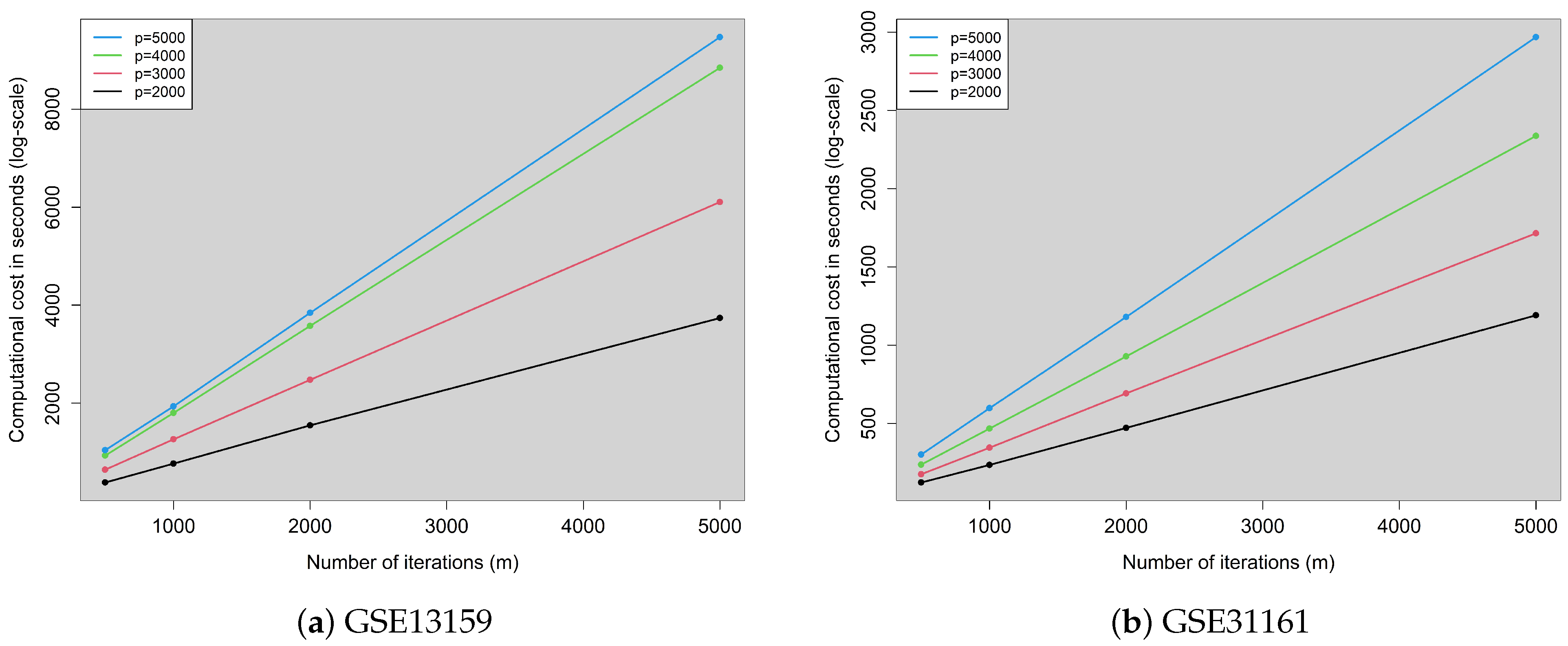
We randomly selected p = 2000, 3000, 4000, and 5000 variables and run the optimized rmdp() function (with parallel computations) 20 times with a varying number of iterations, m (see Step 1), equal to 500, 1000, 2000, and 5000. The purpose of this exercise was dual: first, to evaluate the computational cost with such a high dimensional dataset, and secondly, to assess the effect of the iterations on the stability of the outliers detected. Table 3 contains the relevant results, and Figure 1 visualizes the computational cost.
Table 3.
Computational cost (left, in seconds) and stability (right, in %) in the outliers detected for the GSE13159 and GSE31161 datasets.
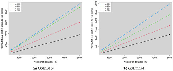
Figure 1.
Computational cost of the rmdp() function with parallel computations as a function of the number of iterations (m) for different dimensionalities. (a) GSE13159. (b) GSE31161.
Table 3 clearly shows that it would be computationally prohibitive to use the original RMDP() with datasets of this size. Figure 1 clearly shows that, regardless of the dataset (and hence sample size), for each dimensionality, the number of iterations m affects the computational cost in a linear manner. However, for every increase in the dimensionality, the computational cost increases at a super-linear rate. This can be claimed for the the sample size as well since the GSE13159 contains almost double the observations GSE31161 contains; however, the time required is more than double. Regarding the stability of the outliers detected, the percentages of agreement are quite high (close to 100%), indicating that the number of iterations does not have an important effect. That is, whether the MDP algorithm is run with or with , the detected outliers will be almost the same, except for 1 or 2 (for sample sizes of the order of 1000 or 2000). This observation, in conjunction with the computational cost, is an important one. Given that the MDP algorithm with requires approximately 10 times more time than and the results are nearly the same, there is no reason to increase the number of iterations m in Step 1.
5. Conclusions
The goal of this short paper was to demonstrate that efficient coding, knowledge of how R operates during mathematical operations, and the use of C++ sometimes are enough to make an algorithm really fast. Mathematical tricks, from linear algebra in our case, are also required to boost the speed of the function. In simple words, the algorithm is important but its implementation is also crucial if one is interested in computational costs. We were able to reduce the computational cost of a computationally demanding algorithm by following the aforementioned suggestions. The results from the experiments showcased a successful application of these suggestions in the high-dimensional setting, a computationally demanding case scenario. Overall, our suggestions lead to tremendous reductions in time, with a speed-up factor ranging from only 17 to more than 1800. That is, our new implementation can be up to 1800 times faster than the original implementation provided by the authors of the algorithm.
Finally, the experiments with real datasets further revealed that the initial implementation of the MDP algorithm would be almost impossible to run with datasets of these dimensions. Secondly, there was evidence that the number of iterations of the algorithm does not seem to affect its stability in the outlier detection, which further assures that the computational cost of the MDP algorithm will not explode, even with the use of the rmdp() function with parallel computation.
We did not compare the MDP algorithm to other competing algorithms because this was outside the scope of the paper. The practical significance of this paper was to reduce the computational cost of a well-established algorithm to make it computationally more affordable and hence scalable. The theoretical soundness and capabilities of the MDP algorithm have been already discussed [3]. Our task was to implement and provide a scalable, fast, and more usable function via R so that researchers can use it.
Finally, we should highlight that the MDP algorithm is not only applicable to gene expression data or bioinformatics data in general, as it can be applied to any case scenario involving high-dimensional data. Further, the tricks presented in this paper can be applied to other problems as well. The use of more computationally efficient functions, the use of R packages that contain faster implementations (perhaps written in C++), and the use of linear algebra tricks, like the one we used, are not exclusively to be applied in our case but can be applied to any problem, regardless of whether the data are high-dimensional or simply multivariate. In other words, a fast algorithm requires programming skills and mathematical skills, and our paper showcases this.
Author Contributions
M.T. conceived the idea and discussed it with A.A. and O.A., M.P. translated the R code to C++, M.T., A.A. and O.A. designed the simulation studies. M.T. wrote the paper with inputs from all other authors. All authors have read and agreed to the published version of the manuscript.
Funding
This research received no external funding.
Data Availability Statement
The GSE data used in the paper are public and can be freely accessed. Reference is given within the manuscript.
Conflicts of Interest
The authors declare no conflict of interest.
References
- Rousseeuw, P.J.; Hubert, M. Robust statistics for outlier detection. Wiley Interdiscip. Rev. Data Min. Knowl. Discov. 2011, 1, 73–79. [Google Scholar] [CrossRef]
- Omar, S.; Ngadi, A.; Jebur, H.H. Machine Learning Techniques for Anomaly Detection: An Overview. Int. J. Comput. Appl. 2013, 79, 33–41. [Google Scholar] [CrossRef]
- Ro, K.; Zou, C.; Wang, Z.; Yin, G. Outlier detection for high-dimensional data. Biometrika 2015, 102, 589–599. [Google Scholar] [CrossRef]
- Rousseeuw, P.J.; Driessen, K.V. A fast algorithm for the minimum covariance determinant estimator. Technometrics 1999, 41, 212–223. [Google Scholar] [CrossRef]
- Papadakis, M.; Tsagris, M.; Dimitriadis, M.; Fafalios, S.; Tsamardinos, I.; Fasiolo, M.; Borboudakis, G.; Burkardt, J.; Zou, C.; Lakiotaki, K.; et al. Rfast: A Collection of Efficient and Extremely Fast R Functions; R Package Version 2.1.0; 2023. Available online: https://cloud.r-project.org/web/packages/Rfast/Rfast.pdf (accessed on 3 September 2024).
- Strang, G. Introduction to Linear Algebra, 6th ed.; Wellesley-Cambridge Press: Wellesley, MA, USA, 2023. [Google Scholar]
- Lakiotaki, K.; Vorniotakis, N.; Tsagris, M.; Georgakopoulos, G.; Tsamardinos, I. BioDataome: A collection of uniformly preprocessed and automatically annotated datasets for data-driven biology. Database 2018, 2018, bay011. [Google Scholar] [CrossRef] [PubMed]
- Fayomi, A.; Pantazis, Y.; Tsagris, M.; Wood, A.T. Cauchy robust principal component analysis with applications to high-dimensional data sets. Stat. Comput. 2024, 34, 26. [Google Scholar] [CrossRef]
Disclaimer/Publisher’s Note: The statements, opinions and data contained in all publications are solely those of the individual author(s) and contributor(s) and not of MDPI and/or the editor(s). MDPI and/or the editor(s) disclaim responsibility for any injury to people or property resulting from any ideas, methods, instructions or products referred to in the content. |
© 2024 by the authors. Licensee MDPI, Basel, Switzerland. This article is an open access article distributed under the terms and conditions of the Creative Commons Attribution (CC BY) license (https://creativecommons.org/licenses/by/4.0/).