Computational Analysis of a Novel Iterative Scheme with an Application

Abstract

The computational study of fixed-point problems in distance spaces is an active and important research area. The purpose of this paper is to construct a new iterative scheme in the setting of Banach space for approximating solutions of fixed-point problems. We first prove the strong convergence of the scheme for a general class of contractions under some appropriate assumptions on the domain and a parameter involved in our scheme. We then study the qualitative aspects of our scheme, such as the stability and order of convergence for the scheme. Some nonlinear problems are then considered and solved numerically by our new iterative scheme. The numerical simulations and graphical visualizations prove the high accuracy and stability of the new fixed-point scheme. Eventually, we solve a 2D nonlinear Volterra Integral Equation (VIE) via the application of our main outcome. Our results improve many related results in fixed-point iteration theory.

1. Introduction

Fixed-point approximation for an operator equation is an active research topic on its own. This is due to the fact that many classes of nonlinear problems are not easy to solve directly [1,2,3,4,5,6,7]. In such cases, the solution to any such type of problem is expressed as a fixed point of a certain linear or nonlinear function with the domain as an appropriate subset of some distance space. Fixed-point theorems are the most fundamental results in analysis that guarantee the existence of unique or non-unique fixed-point solutions for operator equations. Sometimes, it is possible that an operator equation may have a solution but the basic fixed-point method may fail to approximate it. Hence, in such cases, the approximation of the solution is not an easy task. For more details on this in the literature, see [8,9,10,11,12,13] and others.

In recent years, fixed-point theory has experienced rapid growth due to its significant applications in various areas of pure and applied mathematics. Consider a real Banach space ($\mathfrak{B},\left|\right|.\left|\right|$) with $\mathfrak{D}$ as a nonempty, closed, and convex subset of $\mathfrak{B}$. Let $\Gamma :\mathfrak{D}\to \mathfrak{D}$ be a self-mapping on $\mathfrak{D}$, and let $a_0\in \mathfrak{D}$. Then, $a_0$ is called a fixed point for $\Gamma$ if $a_0=\Gamma a_0$. In this paper, we have denoted throughout that $F_{\Gamma }=\{r\in \mathfrak{D}:\Gamma r=r\}$, the fixed point set of $\Gamma$.

For approximating fixed-point solutions, Picard suggested the following iterative scheme in 1880, which reads as follows:

$$a_{n+1}=\Gamma a_n,(\mathrm{where}n=0,1,2,\dots ).$$

(1)

Notice that Picard’s iteration is a fundamental iterative scheme in fixed-point theory that produces an iterative sequence ${\left\{a_n\right\}}_{n=0}^{\infty }$ called the Picard iterative sequence for any initial guess, namely, $a_0\in \mathfrak{D}$.

In 1953, Mann [14] extended the concept of Picard iterative sequences by introducing a more general iterative method as follows:

$$a_{n+1}=(1-{\sigma }_n)a_n+{\sigma }_n\Gamma a_n,(\mathrm{where}n=0,1,2,\dots ),$$

(2)

where the scalar sequence ${\left\{{\sigma }_n\right\}}_{n=0}^{\infty }$ is in the interval $[0, 1]$. As for ${\sigma }_n=1$, the Mann iterative scheme reduces to the Picard one.

In 1974, Ishikawa [15] was the first author who suggested the two-step iterative scheme as follows:

$$\left\{\begin{array}{c}{a}_1\in \mathfrak{D},\hfill \\ b_n=(1-{\theta }_n)a_n+{\theta }_n\Gamma a_n,\hfill \\ a_{n+1}=(1-{\sigma }_n)a_n+{\sigma }_n\Gamma b_n,(\mathrm{where}n=0,1,2,\dots ),\hfill \end{array}\right.$$

(3)

where the scalar sequences ${\left\{{\sigma }_n\right\}}_{n=0}^{\infty }$ and ${\left\{{\theta }_n\right\}}_{n=0}^{\infty }$ are in the interval $[0, 1]$. The Ishikawa iteration can be considered a two-step Mann iteration and includes both Mann and Picard iterative schemes as special cases. For example, for ${\theta }_n=0$, the Ishikawa iteration reduces to the Mann iteration. Recently, numerous researchers have investigated new iterative schemes [14,15,16,17,18,19,20,21,22,23,24,25,26,27,28,29,30,31] containing a number of steps for approximating fixed points of various classes of nonlinear operators and solving operator equations within appropriate classes of distance spaces.

Sometimes, one- and two-step iterations like Picard, Mann, and Ishikawa are not the best option for numerical reckoning of fixed points of some classes of selfmaps due to the slow convergence rates. Hence, in such cases, three-step iterations that are known to converge rapidly to fixed points of many nonlinear mappings are requested. Thus, to achieve this objective, Karakaya [21] in 2017 introduced the following three-step iteration:

$$\left\{\begin{array}{c}{x}_1\in \mathfrak{D},\hfill \\ z_n=\Gamma x_n,\hfill \\ y_n=(1-{\sigma }_n)z_n+{\sigma }_n\Gamma z_n,\hfill \\ x_{n+1}=\Gamma y_n,(\mathrm{where}n=0,1,2,\dots ),\hfill \end{array}\right.$$

(4)

where the scalar sequence ${\left\{{\sigma }_n\right\}}_{n=0}^{\infty }$ is in the interval $[0,1]$.

Keeping the above work in mind, Ullah and Arshad [23] in 2018 constructed a simple three-step iteration called M-iteration as follows:

$$\left\{\begin{array}{c}{x}_1\in \mathfrak{D},\hfill \\ z_n=(1-{\sigma }_n)x_n+{\sigma }_n\Gamma x_n,\hfill \\ y_n=\Gamma z_n,\hfill \\ x_{n+1}=\Gamma y_n,(\mathrm{where}n=0,1,2,\dots ),\hfill \end{array}\right.$$

(5)

where the scalar sequence ${\left\{{\sigma }_n\right\}}_{n=0}^{\infty }$ is in the interval $[0,1]$.

Similarly, Abbas et al. [24] in 2018 studied the following new three-step iteration:

$$\left\{\begin{array}{c}{x}_1\in \mathfrak{D},\hfill \\ z_n=\Gamma x_n,\hfill \\ y_n=\Gamma z_n,\hfill \\ x_{n+1}=(1-{\sigma }_n)y_n+{\sigma }_n\Gamma y_n,(\mathrm{where}n=0,1,2,\dots ),\hfill \end{array}\right.$$

(6)

where the scalar sequence ${\left\{{\sigma }_n\right\}}_{n=0}^{\infty }$ is in the interval $[0,1]$. The authors studied the rate of convergence of the above scheme and compared these convergence rates with all of the above iterations.

It is worth mentioning that all the above iterative schemes are constructed upon the same idea. Thus, to study fixed-point schemes in a new sense, Sharma et al. [28] very recently constructed a new type of iterative scheme that is different in design from all of the above iterative schemes. Their new type of scheme reads as follows:

$$\left\{\begin{array}{c}{a}_1\in \mathfrak{D},\hfill \\ c_n={\displaystyle \frac{\mu a_n+\Gamma a_n}{\mu +1}},\hfill \\ b_n=\Gamma c_n,\hfill \\ a_{n+1}=\Gamma b_n,(\mathrm{where}n=0,1,2,\dots ),\hfill \end{array}\right.$$

(7)

where $\mu >0$ is a real number.

Sharma et al. [28] constructed the above fixed-point scheme by using the idea of Kanwar et al. [20]. The Kanwar et al. [20] scheme reads as follows:

$$a_{n+1}={\displaystyle \frac{\mu a_n+\Gamma a_n}{\mu +1}},(\mathrm{where}n=0,1,2,\dots ),$$

(8)

where the number $\mu \ge 0$, and notice that when $\mu =0$, the above scheme reduces to the case of Picard’s iteration.

In recent years, we have seen that iterative construction under various iterative schemes has attracted many researchers and new fixed-point convergence results have been obtained. Moreover, they suggested new applications of these new outcomes. Motivated by these considerations, we propose a new iterative scheme for solving a wide range of nonlinear problems in Banach spaces. This novel scheme is straightforward and requires minimal initial information. Its primary advantage lies in its simplicity, relying on just a single sequence of scalars while also exhibiting a rapid rate of convergence. Additionally, we explore its application within the framework of 2D Volterra equations.

2. Preliminaries

To prove the main outcome, some basic facts are needed from the present literature. We will use these concepts and results for proving our main results.

The following general concept of mappings is from Zamfirescu [32].

Definition 1. 

Assume that Γ is a selfmap on a Banach space, namely $\mathfrak{B}$. In this case, Γ is called a generalized contraction in the sense of Zamfirescu contraction provided that there are some constants, namely $\sigma ,\theta$, and ξ with $0\le \sigma <1,0\le \theta ,\xi <0.5$ such that for any choice of $a,b\in \mathfrak{B}$, at least one of the following conditions hold:

($c_1$). 

$\left|\right|\Gamma a-\Gamma b\left|\right|\le \sigma \left|\right|a-b\left|\right|$;

($c_2$). 

$\left|\right|\Gamma a-\Gamma b\left|\right|\le \theta \left[\right||a-\Gamma a||+||b-\Gamma b|\left|\right]$;

($c_3$). 

$\left|\right|\Gamma a-\Gamma b\left|\right|\le \xi \left[\right||a-\Gamma b||+||b-\Gamma a|\left|\right]$.

Zamfirescu [32] provided that the mappings from the above class admit a unique fixed point in the setting of complete metric spaces and the fixed point can be approximated by Picard’s iteration (1).

The class of Zamfirescu includes many classical contractions. In [33], Berinde extended the concept of these mappings as follows:

A mapping $\Gamma$ is called a generalized contraction in the sense of Berinde [33] provided that

$$\begin{array}{c}\hfill \left|\right|\Gamma a-\Gamma b\left|\right|\le 2\rho \left|\right|a-\Gamma a\left|\right|+\rho \left|\right|a-b\left|\right|,\end{array}$$

(9)

for every choice of $a,b$ in the normed space $\mathfrak{B}$; here, $\rho =max\{\sigma ,{\displaystyle \frac{\theta }{1-\theta }},{\displaystyle \frac{\xi }{1-\xi }}\},0\le \sigma <1$, with $0\le \theta ,\xi <0.5$.

Following the above concepts, Osilike [34] suggested a new class of mappings that are more general than the class of mappings introduced in [11]. A mapping $\Gamma$ is called a generalized contraction in the sense of Osilike provided that one has constants $L\ge 0$, $\rho \in [0,1)$ for any choice of $a,b$ in the normed space $\mathfrak{B}$, and it follows that

$$\begin{array}{c}\hfill \left|\right|\Gamma a-\Gamma b\left|\right|\le L\left|\right|a-\Gamma a\left|\right|+\rho \left|\right|a-b\left|\right|.\end{array}$$

(10)

Once existence of a fixed point for any self map is obtained, it is needed to compute the fixed point of the given mapping. However, when we approximate the fixed point, stability analysis of the proposed method is also important. In [35], the authors obtained the stability and convergence of basic iterative schemes due to Picard and Mann for mappings related to (10) under the following condition: one has a constant $\rho \in [0,1)$ and a function $\psi$ from $[0,\infty )$ to $[0,\infty )$ such that $\psi \left(0\right)=0$ and $\psi$ are increasing and continuous functions, such that

$$\begin{array}{c}\hfill \left|\right|\Gamma a-\Gamma b\left|\right|\le \psi \left(\right||a-\Gamma a|\left|\right)+\rho \left|\right|a-b\left|\right|,\end{array}$$

(11)

for all points $a,b$ in the normed space $\mathfrak{B}$.

Now to obtain the required fixed point results, we need some basic lemmas.

Lemma 1 

([36]). Assume that we have a sequence ${\left\{{ϵ}_n\right\}}_{n=0}^{\infty }$ composed of positive real numbers such that ${lim}_{n\to \infty }{ϵ}_n=0$, where $\rho \in (0,1)$. In this case, for any other positive real numbers sequence, namely ${\left\{x_n\right\}}_{n=0}^{\infty }$, if one has a property that $x_{n+1}\le {ϵ}_n+\rho x_n$, then ${lim}_{n\to \infty }{x}_n=0$ holds.

Lemma 2 

([37]). Assume that the condition $a_{n+1}\le (1-{\eta }_n)a_n+b_n$ holds for any two sequences ${\left\{a_n\right\}}_{n=0}^{\infty }$, ${\left\{b_n\right\}}_{n=0}^{\infty }$ and $0<{\eta }_n<1$. If one has ${\displaystyle \frac{b_n}{{\eta }_n}}\to 0$ and ${\sum }_{n=0}^{\infty }{\eta }_n=\infty$, then it follows that ${lim}_{n\to \infty }{a}_n=0$.

The following definition is about the stability of an iterative scheme that can be found in [38].

Definition 2. 

A given iterative scheme, namely $a_{n+1}=f(\Gamma ,a_n)$, is known as stable (sometimes called Γ-stable) on a given selfmap $Gamma$ provided that it is convergent to a fixed point r of Γ and the following condition is true for any other sequence, namely $t_n$:

$$\underset{n\to \infty }{lim}{ϵ}_n=0\iff \underset{n\to \infty }{lim}{t}_n=r,$$

where ${ϵ}_n=\left|\right|t_{n+1}-f(\Gamma ,t_n)\left|\right|$.

We can also compare two iterative schemes. The following definition for the comparison of two fixed-point schemes was provided by Berinde [39].

Definition 3. 

If we have two sequences, namely ${\left\{a_n\right\}}_{n=0}^{\infty }$ and ${\left\{b_n\right\}}_{n=0}^{\infty }$, obtained from two iteration schemes and convergent, respectively, to a and b, then, in this case, the first sequence ${\left\{a_n\right\}}_{n=0}^{\infty }$ is known as faster convergent as compared to ${\left\{b_n\right\}}_{n=0}^{\infty }$ when the following condition is held:

$$\underset{n\to \infty }{lim}\left|{\displaystyle \frac{a_n-a}{b_n-b}}\right|=0.$$

Definition 4 

([39]). Assume that we have two sequences, namely ${\left\{x_n\right\}}_{n=0}^{\infty }$ and ${\left\{y_n\right\}}_{n=0}^{\infty }$, that are produced from two different iterations but both converge to a fixed point r. If ${\left\{a_n\right\}}_{n=0}^{\infty }$ and ${\left\{b_n\right\}}_{n=0}^{\infty }$ are two sequences that are convergent to zero, then the error estimates satisfy $\left|\right|x_n-r\left|\right|\le a_n$ and $\left|\right|y_n-r\left|\right|\le b_n$. If the sequence ${\left\{a_n\right\}}_{n=0}^{\infty }$ is faster convergent than ${\left\{b_n\right\}}_{n=0}^{\infty }$, then ${\left\{x_n\right\}}_{n=0}^{\infty }$ is also faster convergent than ${\left\{y_n\right\}}_{n=0}^{\infty }$.

Definition 5 

([33]). Assume that we have sequence ${\left\{a_n\right\}}_{n=0}^{\infty }$ in a Banach space, namely $\mathfrak{B}$. ${\left\{a_n\right\}}_{n=0}^{\infty }$ is strongly convergent to a point r iff ${lim}_{n\to \infty }\left|\right|a_n-r\left|\right|=0$.

3. Novel Iteration and Convergence Results

Assume that $\mathfrak{D}$ is any closed subset of a Banach space. Our new iteration scheme in this case reads as follows:

$$\left\{\begin{array}{c}{a}_1\in \mathfrak{D},\hfill \\ e_n={\displaystyle \frac{\mu a_n+\Gamma a_n}{\mu +1}},\hfill \\ d_n=\Gamma e_n,\hfill \\ c_n=\Gamma d_n,\hfill \\ b_n=\Gamma c_n,\hfill \\ a_{n+1}=\Gamma b_n,(n=1,2,3,\dots ).\hfill \end{array}\right.$$

(12)

where $a_1$ is a starting guess and the scalar $\mu >0$ is a fixed real constant.

Now we are going to provide some convergence results of our new scheme.

Theorem 1. 

Assume that Γ is any selfmap from a convex closed nonempty subset $\mathfrak{D}$ of a Banach space. If Γ satisfies (11) and has a fixed point, namely r, then the sequence ${\left\{a_n\right\}}_{n=0}^{\infty }$ generated in (12) is strongly convergent to the unique fixed point.

Proof. 

We want to show that ${lim}_{n\to \infty }{a}_n=r$. Considering (12), one has

$$\begin{array}{ccc}\hfill \left|\right|e_n-r\left|\right|& =& \left|\right|{\displaystyle \frac{\mu a_n+\Gamma a_n}{\mu +1}}-r\left|\right|\hfill \\ & =& \left|\right|\left({\displaystyle \frac{\mu }{\mu +1}}\right)(a_n-r)+\left({\displaystyle \frac{1}{\mu +1}}\right)(\Gamma a_n-r)\left|\right|\hfill \\ & \le & \left({\displaystyle \frac{\mu }{\mu +1}}\right)\left|\right|a_n-r\left|\right|+\left({\displaystyle \frac{1}{\mu +1}}\right)\left|\right|\Gamma a_n-r\left|\right|\hfill \\ & \le & \left({\displaystyle \frac{\mu }{\mu +1}}\right)\left|\right|a_n-r\left|\right|+\left({\displaystyle \frac{1}{\mu +1}}\right)\left(\psi \right(\left|\right|r-\Gamma r\left|\right|)+\rho \left|\right|r-a_n\left|\right|)\hfill \\ & =& \left({\displaystyle \frac{\mu }{\mu +1}}\right)\left|\right|a_n-r\left|\right|+\left({\displaystyle \frac{\rho }{\mu +1}}\right)\left|\right|a_n-r\left|\right|\hfill \\ & =& \left({\displaystyle \frac{\mu +\rho }{\mu +1}}\right)\left|\right|a_n-r\left|\right|.\hfill \end{array}$$

(13)

Moreover, we have

$$\begin{array}{ccc}\hfill \left|\right|d_n-r\left|\right|& =& \left|\right|\Gamma e_n-r\left|\right|\hfill \\ & =& \left|\right|\Gamma r-\Gamma e_n\left|\right|\hfill \\ & \le & \psi \left(\right||r-\Gamma r\left|\right|)+\rho \left|\right|r-e_n\left|\right|\hfill \\ & =& \rho \left|\right|e_n-r\left|\right|,\hfill \end{array}$$

(14)

$$\begin{array}{ccc}\hfill \left|\right|c_n-r\left|\right|& =& \left|\right|\Gamma d_n-r\left|\right|\hfill \\ & =& \left|\right|\Gamma r-\Gamma d_n\left|\right|\hfill \\ & \le & \psi \left(\right||r-\Gamma r\left|\right|)+\rho \left|\right|r-d_n\left|\right|\hfill \\ & =& \rho \left|\right|d_n-r\left|\right|,\hfill \end{array}$$

(15)

$$\begin{array}{ccc}\hfill \left|\right|b_n-r\left|\right|& =& \left|\right|\Gamma c_n-r\left|\right|\hfill \\ & =& \left|\right|\Gamma r-\Gamma c_n\left|\right|\hfill \\ & \le & \psi \left(\right||r-\Gamma r\left|\right|)+\rho \left|\right|r-c_n\left|\right|\hfill \\ & =& \rho \left|\right|c_n-r\left|\right|,\hfill \end{array}$$

(16)

and

$$\begin{array}{ccc}\hfill \left|\right|a_{n+1}-r\left|\right|& =& \left|\right|\Gamma b_n-r\left|\right|\hfill \\ & =& \left|\right|\Gamma r-\Gamma b_n\left|\right|\hfill \\ & \le & \psi \left(\right||r-\Gamma r\left|\right|)+\rho \left|\right|r-b_n\left|\right|\hfill \\ & =& \rho \left|\right|b_n-r\left|\right|.\hfill \end{array}$$

(17)

Substituting (14)–(16) in (17), we have

$$\begin{array}{ccc}\hfill \left|\right|a_{n+1}-r\left|\right|& \le & {\rho }^4\left|\right|e_n-r\left|\right|.\hfill \end{array}$$

(18)

From (13) in (18), one has

$$\begin{array}{ccc}\hfill \left|\right|a_{n+1}-r\left|\right|& \le & {\rho }^4\left({\displaystyle \frac{\mu +\rho }{\mu +1}}\right)\left|\right|a_n-r\left|\right|.\hfill \end{array}$$

(19)

Again, it follows that

$$\begin{array}{ccc}\hfill \left|\right|a_n-r\left|\right|& \le & {\rho }^4\left({\displaystyle \frac{\mu +\rho }{\mu +1}}\right)\left|\right|a_{n-1}-r\left|\right|\hfill \\ \hfill \left|\right|a_{n-1}-r\left|\right|& \le & {\rho }^4\left({\displaystyle \frac{\mu +\rho }{\mu +1}}\right)\left|\right|a_{n-2}-r\left|\right|\hfill \\ \hfill .\\ \hfill .\\ \hfill .\\ \hfill \left|\right|a_1-r\left|\right|& \le & {\rho }^4\left({\displaystyle \frac{\mu +\rho }{\mu +1}}\right)\left|\right|a_0-r\left|\right|.\hfill \end{array}$$

From the above inequalities, we obtain

$$\begin{array}{ccc}\hfill \left|\right|a_{n+1}-r\left|\right|& \le & {\rho }^{4(n+1)}{\left({\displaystyle \frac{\mu +\rho }{\mu +1}}\right)}^{n+1}\left|\right|a_0-r\left|\right|.\hfill \end{array}$$

(20)

As $\rho <1$, then $\mu +\rho <\mu +1$, $0<{\displaystyle \frac{\mu +\rho }{\mu +1}}<1$, which implies that

$${\rho }^{4(n+1)}{\left({\displaystyle \frac{\mu +\rho }{\mu +1}}\right)}^{n+1}\to 0$$

as $n\to \infty$.

Now we see from (20) that ${lim}_{n\to \infty }\left|\right|a_{n+1}-r\left|\right|=0$. Eventually, this shows that $\left\{a_n\right\}$ is strongly convergent to r.

It remains to show that the fixed point of $\Gamma$ is unique. For this, we take two fixed points of r, $r^{*}$ of $\Gamma$, that is, $\Gamma r=\Gamma r^{*}=r$ with $r\ne r^{*}$. Then, we have

$$\begin{array}{ccc}\hfill \left|\right|r-r^{*}\left|\right|& =& \left|\right|\Gamma r-\Gamma r^{*}\left|\right|\hfill \\ & \le & \psi \left(\right||r-\Gamma r\left|\right|)+\rho \left|\right|r-r^{*}\left|\right|\hfill \\ & =& \rho \left|\right|r-r^{*}\left|\right|\hfill \\ & <& \left|\right|r-r^{*}\left|\right|,\hfill \end{array}$$

but $\rho <1$. This is a contradiction, and hence, $r=r^{*}$. □

Theorem 2. 

Assume that Γ is any selfmap from a convex closed nonempty subset $\mathfrak{D}$ of a Banach space. If Γ satisfies (11) and has a fixed point, namely r, then the sequence ${\left\{a_n\right\}}_{n=0}^{\infty }$ generated in (12) is strongly convergent to the unique fixed point and the convergence is Γ-stable.

Proof. 

The first part follows from the last theorem. To prove the other part, we may take another sequence ${\left\{t_n\right\}}_{n=0}^{\infty }$ and assume that $a_{n+1}=f(\Gamma ,a_n)$ is convergent to r. Suppose ${ϵ}_n=\left|\right|t_{n+1}-f(\Gamma ,t_n)\left|\right|$. We need to prove that ${lim}_{n\to \infty }{ϵ}_n=0$ iff ${lim}_{n\to \infty }{t}_n=r$. First, we assume that ${lim}_{n\to \infty }{ϵ}_n=0$, and we have

$$\begin{array}{ccc}\hfill \left|\right|t_{n+1}-r\left|\right|& =& \left|\right|t_{n+1}-f(\Gamma ,t_n)+f(\Gamma ,t_n)-r\left|\right|\hfill \\ & \le & \left|\right|t_{n+1}-f(\Gamma ,t_n)\left|\right|+\left|\right|f(\Gamma ,t_n)-r\left|\right|\hfill \\ & =& {ϵ}_n+\left|\right|f(\Gamma ,t_n)-r\left|\right|\hfill \\ & =& {ϵ}_n+\left|\right|\Gamma (\Gamma (\Gamma (\Gamma ({\displaystyle \frac{\mu t_n+\Gamma t_n}{\mu +1}}))))-r\left|\right|\hfill \\ & =& {ϵ}_n+\left|\right|\Gamma r-\Gamma (\Gamma (\Gamma (\Gamma ({\displaystyle \frac{\mu t_n+\Gamma t_n}{\mu +1}}))))\left|\right|\hfill \\ & \le & {ϵ}_n+\rho \left|\right|r-\Gamma (\Gamma (\Gamma ({\displaystyle \frac{\mu t_n+\Gamma t_n}{\mu +1}})))\left|\right|\hfill \\ & =& {ϵ}_n+\rho \left|\right|\Gamma r-\Gamma (\Gamma (\Gamma ({\displaystyle \frac{\mu t_n+\Gamma t_n}{\mu +1}})))\left|\right|\hfill \\ & \le & {ϵ}_n+{\rho }^2\left|\right|r-\Gamma (\Gamma ({\displaystyle \frac{\mu t_n+\Gamma t_n}{\mu +1}}))\left|\right|\hfill \\ & =& {ϵ}_n+{\rho }^2\left|\right|\Gamma r-\Gamma (\Gamma ({\displaystyle \frac{\mu t_n+\Gamma t_n}{\mu +1}}))\left|\right|\hfill \\ & \le & {ϵ}_n+{\rho }^3\left|\right|r-\Gamma ({\displaystyle \frac{\mu t_n+\Gamma t_n}{\mu +1}})\left)\right||\hfill \\ & =& {ϵ}_n+{\rho }^3\left|\right|\Gamma r-\Gamma ({\displaystyle \frac{\mu t_n+\Gamma t_n}{\mu +1}}))||\hfill \\ & \le & {ϵ}_n+{\rho }^4\left|\right|r-({\displaystyle \frac{\mu t_n+\Gamma t_n}{\mu +1}})\left|\right|\hfill \\ & =& {ϵ}_n+{\rho }^4\left|\right|({\displaystyle \frac{\mu }{\mu +1}})(r-t_n)+({\displaystyle \frac{1}{\mu +1}})(r-\Gamma t_n)\left|\right|\hfill \\ & \le & {ϵ}_n+{\rho }^4(({\displaystyle \frac{\mu }{\mu +1}})\left|\right|r-t_n\left|\right|+({\displaystyle \frac{1}{\mu +1}})\left|\right|\Gamma r-\Gamma t_n\left|\right|)\hfill \\ & \le & {ϵ}_n+{\rho }^4(({\displaystyle \frac{\mu }{\mu +1}})\left|\right|r-t_n\left|\right|+({\displaystyle \frac{1}{\mu +1}})(\psi (\left|\right|r-\Gamma r\left|\right|)+\rho \left|\right|r-t_n\left|\right|))\hfill \\ & \le & {ϵ}_n+{\displaystyle \frac{{\rho }^4(\mu +\rho )}{\mu +1}}\left|\right|t_n-r\left|\right|.\hfill \end{array}$$

Notice that ${\displaystyle \frac{{\rho }^4(\mu +\rho )}{\mu +1}}<1$ and ${lim}_{n\to \infty }{ϵ}_n=0$; according to Lemma 1, it follows that ${lim}_{n\to \infty }{t}_n=r$.

Conversely, we consider that ${lim}_{n\to \infty }{t}_n=r$ is held. Now, we have

$$\begin{array}{ccc}\hfill {ϵ}_n& =& \left|\right|t_{n+1}-f(\Gamma ,t_n)\left|\right|\hfill \\ & =& \left|\right|t_{n+1}-r+r-f(\Gamma ,t_n)\left|\right|\hfill \\ & \le & \left|\right|t_{n+1}-r\left|\right|+\left|\right|f(\Gamma ,t_n)-r\left|\right|\hfill \\ & \le & \left|\right|t_{n+1}-r\left|\right|+{\displaystyle \frac{{\rho }^4(\mu +\rho )}{\mu +1}}\left|\right|t_n-r\left|\right|.\hfill \end{array}$$

However, ${lim}_{n\to \infty }{t}_n=r$ holds, and it follows that ${lim}_{n\to \infty }{ϵ}_n=0$. Subsequently, the convergence of the scheme defined in (12) is essentially $\Gamma$-stable. □

Theorem 3. 

If ${\left\{a_n\right\}}_{n=0}^{\infty }$ and ${\left\{x_n\right\}}_{n=0}^{\infty }$ are produced from (12) and (5), respectively, and both are convergent to a unique fixed point of Γ, then ${\left\{a_n\right\}}_{n=0}^{\infty }$ is faster convergent to the fixed point as compared to ${\left\{x_n\right\}}_{n=0}^{\infty }$.

Proof. 

Keeping in mind (20) of Theorem 1, it follows that

$$\begin{array}{ccc}\hfill \left|\right|a_{n+1}-r\left|\right|& \le & {\rho }^{4(n+1)}{\left({\displaystyle \frac{\mu +\rho }{\mu +1}}\right)}^{n+1}\left|\right|a_0-r\left|\right|.\hfill \end{array}$$

(21)

Thus, from iteration scheme (5), one has

$$\begin{array}{ccc}\hfill \left|\right|z_n-r\left|\right|& =& \left|\right|(1-{\sigma }_n)x_n+{\sigma }_n\Gamma x_n-r\left|\right|\hfill \\ & =& \left|\right|(1-{\sigma }_n)x_n+{\sigma }_n\Gamma x_n-{\sigma }_{n}r+{\sigma }_{n}r-r\left|\right|\hfill \\ & =& \left|\right|(1-{\sigma }_n)(x_n-r)+{\sigma }_n(\Gamma x_n-r)\left|\right|\hfill \\ & \le & (1-{\sigma }_n)\left|\right|x_n-r\left|\right|+{\sigma }_n\left|\right|\Gamma r-\Gamma x_n\left)\right||\hfill \\ & \le & (1-{\sigma }_n)\left|\right|x_n-r\left|\right|+{\sigma }_n\left(\psi \right(\left|\right|r-\Gamma r\left|\right|)+\rho \left|\right|r-x_n\left|\right|)\hfill \\ & =& (1-{\sigma }_n)\left|\right|x_n-r\left|\right|+{\sigma }_n\rho \left|\right|x_n-r\left|\right|\hfill \\ & =& (1-(1-\rho ){\sigma }_n)\left|\right|x_n-r\left|\right|.\hfill \end{array}$$

It follows that

$$\begin{array}{ccc}\hfill \left|\right|y_n-r\left|\right|& =& \left|\right|\Gamma z_n-r\left|\right|\hfill \\ & =& \left|\right|\Gamma r-\Gamma z_n\left|\right|\hfill \\ & \le & \psi \left(\right||r-\Gamma r\left|\right|)+\rho \left|\right|r-z_n\left|\right|\hfill \\ & =& \rho \left|\right|z_n-r\left|\right|\hfill \\ & =& \rho (1-(1-\rho ){\sigma }_n)\left|\right|x_n-r\left|\right|,\hfill \end{array}$$

so

$$\begin{array}{ccc}\hfill \left|\right|x_{n+1}-r\left|\right|& =& \left|\right|\Gamma y_n-r\left|\right|\hfill \\ & =& \left|\right|\Gamma r-\Gamma y_n\left|\right|\hfill \\ & \le & \psi \left(\right||r-\Gamma r\left|\right|)+\rho \left|\right|r-y_n\left|\right|\hfill \\ & =& \rho \left|\right|y_n-r\left|\right|\hfill \\ & =& {\rho }^2(1-(1-\rho ){\sigma }_n)\left|\right|x_n-r\left|\right|.\hfill \end{array}$$

Again, one has

$$\begin{array}{ccc}\hfill \left|\right|x_n-r\left|\right|& \le & {\rho }^2(1-(1-\rho ){\sigma }_n)\left|\right|x_{n-1}-r\left|\right|\hfill \\ \hfill \left|\right|x_{n-1}-r\left|\right|& \le & {\rho }^2(1-(1-\rho ){\sigma }_n)\left|\right|x_{n-2}-r\left|\right|\hfill \\ \hfill .\\ \hfill .\\ \hfill .\\ \hfill \left|\right|x_1-r\left|\right|& \le & {\rho }^2(1-(1-\rho ){\sigma }_n)\left|\right|x_0-r\left|\right|\hfill \end{array}$$

From the above, it follows that

$$\begin{array}{ccc}\hfill \left|\right|x_{n+1}-r\left|\right|& \le & {\rho }^{2(n+1)}\prod _{k=0}^n(1-(1-\rho ){\sigma }_k)\left|\right|x_0-r\left|\right|.\hfill \end{array}$$

(22)

However, ${\sigma }_0\le {\sigma }_k<1$, and we have $1-(1-\rho ){\sigma }_k\le 1-(1-\rho ){\sigma }_0$, hence

$$\begin{array}{c}\hfill \prod _{k=0}^n(1-(1-\rho ){\sigma }_k)\le {(1-(1-\rho ){\sigma }_0)}^{n+1}.\end{array}$$

(23)

From (23) in (22), one has

$$\begin{array}{ccc}\hfill \left|\right|x_{n+1}-r\left|\right|& \le & {\rho }^{2(n+1)}{(1-(1-\rho ){\sigma }_0)}^{n+1}\left|\right|x_0-r\left|\right|.\hfill \end{array}$$

(24)

Define

$A_n={\rho }^{4(n+1)}{\left({\displaystyle \frac{\mu +\rho }{\mu +1}}\right)}^{n+1}\left|\right|a_0-r\left|\right|$,

$B_n={\rho }^{2(n+1)}{(1-(1-\rho ){\sigma }_0)}^{n+1}\left|\right|x_0-r\left|\right|$, and

$${{\rm Y}}_n={\displaystyle \frac{A_n}{B_n}}={\displaystyle \frac{{\rho }^{4(n+1)}{\left(\frac{\mu +\rho }{\mu +1}\right)}^{n+1}\left|\right|a_0-r\left|\right|}{{\rho }^{2(n+1)}{(1-(1-\rho ){\sigma }_0)}^{n+1}\left|\right|x_0-r\left|\right|}}.$$

(25)

Using $x_0=a_0$ in (25), we have

$${{\rm Y}}_n={\displaystyle \frac{A_n}{B_n}}={\rho }^2{\left({\displaystyle \frac{\frac{\mu +\rho }{\mu +1}}{1-(1-\rho ){\sigma }_0}}\right)}^{n+1}.$$

Using ${\sigma }_0(\mu +1)<1$, we obtain $1-(1-\rho ){\sigma }_0>{\displaystyle \frac{\mu +\rho }{\mu +1}}$, and it follows that

$${\displaystyle \frac{\frac{\mu +\rho }{\mu +1}}{1-(1-\rho ){\sigma }_0}}<1.$$

Hence, ${lim}_{n\to \infty }{{\rm Y}}_n=0.$ In the view of Definitions (3) and (4), it follows that ${\left\{a_n\right\}}_{n=0}^{\infty }$ is convergent at a faster rate than ${\left\{x_n\right\}}_{n=0}^{\infty }$. □

Remark 1. 

Under the same calculations, one can show that our new scheme (12) is also faster convergent than (4) and (6).

Theorem 4. 

Under the last theorem conditions, assume that ${\left\{a_n\right\}}_{n=0}^{\infty }$ is the sequence of our new iteration (12) and ${\left\{x_n\right\}}_{n=0}^{\infty }$ is the sequence of the Mann iteration suggested in (2). In this case, the following hold.

(i) 

Mann sequence (2) is convergent to the fixed point.

(ii) 

New iteration sequence (12) is convergent to the fixed point.

Proof. 

Assume that the Mann iterative scheme is convergent to the fixed point r, that is, ${lim}_{n\to \infty }\left|\right|x_n-r\left|\right|=0.$ Hence, using (12), one has

$$\begin{array}{ccc}\hfill \left|\right|x_{n+1}-a_{n+1}\left|\right|& =& \left|\right|(1-{\sigma }_n)x_n+{\sigma }_n\Gamma x_n-\Gamma b_n\left|\right|\hfill \\ & =& \left|\right|(1-{\sigma }_n)x_n+{\sigma }_n\Gamma x_n-{\sigma }_n\Gamma b_n+{\sigma }_n\Gamma b_n-\Gamma b_n\left|\right|\hfill \\ & =& \left|\right|(1-{\sigma }_n)x_n-(1-{\sigma }_n)\Gamma b_n+{\sigma }_n(\Gamma x_n-\Gamma b_n)\left|\right|\hfill \\ & \le & (1-{\sigma }_n)\left|\right|x_n-\Gamma b_n\left|\right|+{\sigma }_n\left|\right|\Gamma x_n-\Gamma b_n\left|\right|\hfill \\ & =& (1-{\sigma }_n)\left|\right|x_n-\Gamma x_n+\Gamma x_n-\Gamma b_n\left|\right|+{\sigma }_n\left|\right|\Gamma x_n-\Gamma b_n\left|\right|\hfill \\ & \le & (1-{\sigma }_n)\left|\right|x_n-\Gamma x_n\left|\right|+(1-{\sigma }_n)\left|\right|\Gamma x_n-\Gamma b_n\left|\right|+{\sigma }_n\left|\right|\Gamma x_n-\Gamma b_n\left|\right|\hfill \\ & =& \left|\right|\Gamma x_n-\Gamma b_n\left|\right|+(1-{\sigma }_n)\left|\right|x_n-\Gamma x_n\left|\right|\hfill \\ & \le & \left(\rho \right||x_n-b_n\left|\right|+\psi \left(\right||x_n-\Gamma x_n\left|\right|\left)\right)+(1-{\sigma }_n)\left|\right|x_n-\Gamma x_n\left|\right|.\hfill \end{array}$$

(26)

Moreover, we have

$$\begin{array}{ccc}\hfill \left|\right|x_n-b_n\left|\right|& =& \left|\right|x_n-\Gamma c_n\left|\right|\hfill \\ & =& \left|\right|x_n-\Gamma x_n+\Gamma x_n-\Gamma c_n\left|\right|\hfill \\ & \le & \left|\right|x_n-\Gamma x_n\left|\right|+\left|\right|\Gamma x_n-\Gamma c_n\left|\right|\hfill \\ & \le & \left|\right|x_n-\Gamma x_n\left|\right|+\psi \left(\right||x_n-\Gamma x_n\left|\right|)+\rho \left|\right|x_n-c_n\left|\right|\hfill \\ & =& \left|\right|x_n-\Gamma x_n\left|\right|+\psi \left(\right||x_n-\Gamma x_n\left|\right|)+\rho \left|\right|x_n-\Gamma d_n\left|\right|\hfill \\ & \le & \left|\right|x_n-\Gamma x_n\left|\right|+\psi \left(\right||x_n-\Gamma x_n\left|\right|)+\rho \left(\psi \right(\left|\right|x_n-\Gamma x_n\left|\right|)+\rho \left|\right|x_n-d_n\left|\right|)\hfill \\ & =& \left|\right|x_n-\Gamma x_n\left|\right|+(1+\rho )\psi \left(\right||x_n-\Gamma x_n\left|\right|)+{\rho }^2\left|\right|x_n-d_n\left|\right|\hfill \\ & =& \left|\right|x_n-\Gamma x_n\left|\right|+(1+\rho )\psi \left(\right||x_n-\Gamma x_n\left|\right|)+{\rho }^2\left|\right|x_n-\Gamma e_n\left|\right|\hfill \\ & \le & \left|\right|x_n-\Gamma x_n\left|\right|+(1+\rho )\psi \left(\right||x_n-\Gamma x_n\left|\right|)+{\rho }^2\left(\psi \right(\left|\right|x_n-\Gamma x_n\left|\right|)+\rho \left|\right|x_n-e_n\left|\right|)\hfill \\ & =& \left|\right|x_n-\Gamma x_n\left|\right|+(1+\rho +{\rho }^2)\psi \left(\right||x_n-\Gamma x_n\left|\right|)+{\rho }^3\left|\right|x_n-e_n\left|\right|),\hfill \end{array}$$

(27)

and

$$\begin{array}{ccc}\hfill \left|\right|x_n-e_n\left|\right|& =& \left|\right|x_n-{\displaystyle \frac{\mu a_n+\Gamma a_n}{\mu +1}}\left|\right|\hfill \\ & =& \left|\right|({\displaystyle \frac{\mu }{\mu +1}})(x_n-a_n)+({\displaystyle \frac{1}{\mu +1}})(x_n-\Gamma a_n)\left|\right|\hfill \\ & \le & ({\displaystyle \frac{\mu }{\mu +1}})\left|\right|x_n-a_n\left|\right|+({\displaystyle \frac{1}{\mu +1}})\left|\right|x_n-\Gamma a_n\left|\right|\hfill \\ & =& ({\displaystyle \frac{\mu }{\mu +1}})\left|\right|x_n-a_n\left|\right|+({\displaystyle \frac{1}{\mu +1}})\left|\right|x_n-\Gamma x_n\left|\right|+({\displaystyle \frac{1}{\mu +1}})\left|\right|\Gamma x_n-\Gamma a_n\left|\right|\hfill \\ & \le & ({\displaystyle \frac{\mu }{\mu +1}})\left|\right|x_n-a_n\left|\right|+({\displaystyle \frac{1}{\mu +1}})\left|\right|x_n-\Gamma x_n\left|\right|+({\displaystyle \frac{1}{\mu +1}})(\psi (\left|\right|x_n-\Gamma x_n\left|\right|)+\hfill \\ & & \rho \left|\right|x_n-a_n\left|\right|)\hfill \\ & =& ({\displaystyle \frac{\mu +\rho }{\mu +1}})\left|\right|x_n-a_n\left|\right|+({\displaystyle \frac{1}{\mu +1}})\left|\right|x_n-\Gamma x_n\left|\right|+\hfill \\ & & ({\displaystyle \frac{1}{\mu +1}})\psi (||x_n-\Gamma x_n\left|\right|).\hfill \end{array}$$

(28)

Using (28) in (27), we obtain

$$\begin{array}{ccc}\hfill \left|\right|x_n-b_n\left|\right|& \le & \left|\right|x_n-\Gamma x_n\left|\right|+\psi (1-\rho +{\rho }^2)\left|\right|x_n-\Gamma x_n\left|\right|+\hfill \\ & & {\rho }^3(({\displaystyle \frac{\mu +\rho }{\mu +1}})\left|\right|x_n-a_n\left|\right|+({\displaystyle \frac{1}{\mu +1}})\left|\right|x_n-\Gamma x_n\left|\right|+({\displaystyle \frac{1}{\mu +1}})\psi (||x_n-\Gamma x_n\left|\right|)\hfill \\ & =& {\displaystyle \frac{{\rho }^3(\mu +\rho )}{\mu +1}}\left|\right|x_n-a_n\left|\right|+(1+{\displaystyle \frac{{\rho }^3}{\mu +1}})\left|\right|x_n-\Gamma x_n\left|\right|+\hfill \\ & & ((1-\rho +{\rho }^2)+{\displaystyle \frac{{\rho }^3}{\mu +1}})\psi (||x_n-\Gamma x_n\left|\right|).\hfill \end{array}$$

(29)

Substituting (29) in (26), we obtain

$$\begin{array}{ccc}\hfill \left|\right|x_{n+1}-a_{n+1}\left|\right|& \le & (\rho ({\displaystyle \frac{{\rho }^3(\mu +\rho )}{\mu +1}}\left|\right|x_n-a_n\left|\right|+(1+{\displaystyle \frac{{\rho }^3}{\mu +1}})\hfill \\ & & \left|\right|x_n-\Gamma x_n\left|\right|+((1-\rho +{\rho }^2)+{\displaystyle \frac{{\rho }^3}{\mu +1}})\psi (||x_n-\Gamma x_n\left|\right|)))\hfill \\ & & +\rho \psi (||x_n-\Gamma x_n\left|\right|)+(1-{\sigma }_n)\left|\right|x_n-\Gamma x_n\left|\right|\hfill \\ & =& ({\displaystyle \frac{{\rho }^4(\mu +\rho )}{\mu +1}}||x_n-a_n||+\rho (1+{\displaystyle \frac{{\rho }^3}{\mu +1}})||x_n-\Gamma x_n||+\hfill \\ & & \rho ((1-\rho +{\rho }^2)+{\displaystyle \frac{{\rho }^3}{\mu +1}})\psi (||x_n-\Gamma x_n\left|\right|))+\rho \psi (||x_n-\Gamma x_n\left|\right|)\hfill \\ & & +(1-{\sigma }_n)\left|\right|x_n-\Gamma x_n\left|\right|\hfill \\ & \le & ({\displaystyle \frac{\mu +\rho }{\mu +1}})\left|\right|x_n-a_n\left|\right|+(1+(1-\rho +{\rho }^2)+{\displaystyle \frac{{\rho }^3}{\mu +1}})\psi (||x_n-\Gamma x_n\left|\right|)+\hfill \\ & & ((1-{\sigma }_n)+\rho (1+{\displaystyle \frac{{\rho }^3}{\mu +1}}))\left|\right|x_n-\Gamma x_n\left|\right|.\hfill \end{array}$$

(30)

Let

${\mu }^{*}={\displaystyle \frac{1-\rho }{\mu +1}}\in (0,1)$,

$A_n=\left|\right|x_n-a_n\left|\right|$,

$B_n=(1+(1-\rho +{\rho }^2)+{\displaystyle \frac{{\rho }^3}{\mu +1}})\psi (||x_n-\Gamma x_n\left|\right|)+((1-{\sigma }_n)+\rho (1+{\displaystyle \frac{{\rho }^3}{\mu +1}}))\left|\right|x_n-\Gamma x_n\left|\right|.$ Now

$$\begin{array}{ccc}\hfill \left|\right|x_n-\Gamma x_n\left|\right|& =& \left|\right|x_n-r+\Gamma r-\Gamma x_n\left|\right|\hfill \\ & \le & \left|\right|x_n-r\left|\right|+\left|\right|\Gamma r-\Gamma x_n\left|\right|\hfill \\ & \le & \left|\right|x_n-r\left|\right|+\rho \left|\right|r-x_n\left|\right|+\psi \left(\right||r-\Gamma r\left|\right|)\hfill \\ & =& (1+\rho )\left|\right|x_n-r\left|\right|\to 0\hfill \end{array}$$

when $n\to \infty$. Thus, ${lim}_n\to \infty \left(\psi \right(\left|\right|x_n-\Gamma x_n\left|\right|\left)\right)=\psi ({lim}_n\to \infty \left|\right|x_n-\Gamma x_n\left|\right|)=0$. It follows that $B_n\to 0$. From (30), according to Lemma 2, one has $\left|\right|x_n-a_n\left|\right|\to 0$. Eventually, we found $\left|\right|a_n-r\left|\right|\le \left|\right|a_n-x_n\left|\right|+\left|\right|x_n-r\left|\right|\to 0$. Thus, our scheme produced by (12) is strongly convergent to the fixed point.

On the other side, we may assume that the scheme produced by (12) is strongly convergent to the fixed point r. Hence, ${lim}_n\to \infty \left|\right|a_n-r\left|\right|=0$. Thus, one has

$$\begin{array}{ccc}\hfill \left|\right|a_{n+1}-x_{n+1}\left|\right|& =& \left|\right|\Gamma b_n-(1-{\sigma }_n)x_n-{\sigma }_n\Gamma x_n\left|\right|\hfill \\ & =& \left|\right|\Gamma b_n-(1-{\sigma }_n)x_n+{\sigma }_n\Gamma b_n-{\sigma }_n\Gamma b_n-{\sigma }_n\Gamma x_n\left|\right|\hfill \\ & =& \left|\right|(1-{\sigma }_n)\Gamma b_n-(1-{\sigma }_n)x_n+{\sigma }_n(\Gamma b_n-\Gamma x_n)\left|\right|\hfill \\ & \le & (1-{\sigma }_n)\left|\right|\Gamma b_n-x_n\left|\right|+{\sigma }_n\left|\right|\Gamma b_n-\Gamma x_n\left|\right|\hfill \\ & =& (1-{\sigma }_n)\left|\right|\Gamma b_n-b_n+b_n-x_n\left|\right|+{\sigma }_n\left|\right|\Gamma x_n-\Gamma b_n\left|\right|\hfill \\ & \le & (1-{\sigma }_n)\left|\right|\Gamma b_n-b_n\left|\right|+(1-{\sigma }_n)\left|\right|b_n-x_n\left|\right|+{\sigma }_n\left(\rho \right||b_n-x_n\left|\right|+\hfill \\ & & \psi \left(\right||b_n-\Gamma b_n|\left|\right))\hfill \\ & =& (1-(1-\rho ){\sigma }_n)\left|\right|b_n-x_n\left|\right|+(1-{\sigma }_n)\left|\right|\Gamma b_n-b_n\left|\right|+\hfill \\ & & {\sigma }_n\psi \left(\right||\Gamma b_n-b_n\left|\right|).\hfill \end{array}$$

(31)

Now, we have

$$\begin{array}{ccc}\hfill \left|\right|b_n-x_n\left|\right|& =& \left|\right|\Gamma c_n-x_n\left|\right|\hfill \\ & \le & \left|\right|\Gamma c_n-c_n\left|\right|+\left|\right|c_n-x_n\left|\right|\hfill \\ & =& \left|\right|\Gamma c_n-c_n\left|\right|+\left|\right|\Gamma d_n-x_n\left|\right|\hfill \\ & \le & \left|\right|\Gamma c_n-c_n\left|\right|+\left|\right|\Gamma d_n-d_n\left|\right|+\left|\right|d_n-x_n\left|\right|\hfill \\ & =& \left|\right|\Gamma c_n-c_n\left|\right|+\left|\right|\Gamma d_n-d_n\left|\right|+\left|\right|\Gamma e_n-x_n\left|\right|\hfill \\ & \le & \left|\right|\Gamma c_n-c_n\left|\right|+\left|\right|\Gamma d_n-d_n\left|\right|+\left|\right|\Gamma e_n-e_n\left|\right|+\left|\right|e_n-x_n\left|\right|,\hfill \end{array}$$

(32)

and

$$\begin{array}{ccc}\hfill \left|\right|e_n-x_n\left|\right|& =& \left|\right|{\displaystyle \frac{\mu a_n+\Gamma a_n}{\mu +1}}-x_n\left|\right|\hfill \\ & =& \left|\right|({\displaystyle \frac{\mu }{\mu +1}})a_n+({\displaystyle \frac{1}{\mu +1}})\Gamma a_n-x_n\left|\right|\hfill \\ & \le & ({\displaystyle \frac{\mu }{\mu +1}})\left|\right|x_n-a_n\left|\right|+({\displaystyle \frac{1}{\mu +1}})\left|\right|\Gamma a_n-x_n\left|\right|\hfill \\ & \le & ({\displaystyle \frac{\mu }{\mu +1}})\left|\right|a_n-x_n\left|\right|+({\displaystyle \frac{1}{\mu +1}})\left|\right|\Gamma a_n-a_n\left|\right|+{\displaystyle \frac{1}{\mu +1}}\left|\right|a_n-x_n\left|\right|\hfill \\ & =& \left|\right|a_n-x_n\left|\right|+({\displaystyle \frac{1}{\mu +1}})\left|\right|\Gamma a_n-a_n\left|\right|.\hfill \end{array}$$

(33)

Using (33) in (32), we obtain

$$\begin{array}{ccc}\hfill \left|\right|b_n-x_n\left|\right|& \le & \left|\right|\Gamma c_n-c_n\left|\right|+\left|\right|\Gamma d_n-d_n\left|\right|+\left|\right|\Gamma e_n-e_n\left|\right|+\left|\right|a_n-x_n\left|\right|+({\displaystyle \frac{1}{\mu +1}})\left|\right|\Gamma a_n-a_n\left|\right|.\hfill \end{array}$$

(34)

Substituting (34) in (31), we obtain

$$\begin{array}{ccc}\hfill \left|\right|a_{n+1}-x_{n+1}\left|\right|& \le & (1-(1-\rho ){\sigma }_n)\left(\right||\Gamma c_n-c_n\left|\right|+\left|\right|\Gamma d_n-d_n\left|\right|+\left|\right|\Gamma e_n-e_n\left|\right|+\hfill \\ & & \left|\right|a_n-x_n\left|\right|+({\displaystyle \frac{1}{\mu +1}})\left|\right|\Gamma a_n-a_n\left|\right|)+(1-{\sigma }_n)\left|\right|\Gamma b_n-b_n\left|\right|\hfill \\ & & +{\sigma }_n\psi \left(\right||\Gamma b_n-b_n\left|\right|)\hfill \\ & \le & (1-(1-\rho ){\sigma }_n)\left|\right|a_n-x_n\left|\right|+(1-(1-\rho ){\sigma }_n)\left|\right|\Gamma e_n-e_n\left|\right|+\hfill \\ & & (1-(1-\rho ){\sigma }_n)\left|\right|\Gamma d_n-d_n\left|\right|+(1-(1-\rho ){\sigma }_n)\left|\right|\Gamma c_n-c_n\left|\right|+\hfill \\ & & (1-(1-\rho ){\sigma }_n)({\displaystyle \frac{1}{\mu +1}})\left|\right|\Gamma a_n-a_n\left|\right|)+(1-{\sigma }_n)\left|\right|\Gamma b_n-b_n\left|\right|\hfill \\ & & +{\sigma }_n\psi \left(\right||\Gamma b_n-b_n\left|\right|).\hfill \end{array}$$

(35)

Denote ${\mu }^{*}=(1-\rho ){\sigma }_n\in (0,1)$,

$A_n=\left|\right|a_n-x_n\left|\right|$,

$B_n=(1-(1-\rho ){\sigma }_n)\left|\right|\Gamma e_n-e_n\left|\right|+(1-(1-\rho ){\sigma }_n)\left|\right|\Gamma d_n-d_n\left|\right|+(1-(1-\rho ){\sigma }_n)\left|\right|\Gamma c_n$

$-c_n\left|\right|+(1-(1-\rho ){\sigma }_n)({\displaystyle \frac{1}{\mu +1}})\left|\right|\Gamma a_n-a_n\left|\right|)+(1-{\sigma }_n)\left|\right|\Gamma b_n-b_n\left|\right|+{\sigma }_n\psi \left(\right||\Gamma b_n-b_n\left|\right|)$.

Now, we establish that

$$\begin{array}{ccc}\hfill \left|\right|\Gamma a_n-a_n\left|\right|& =& \left|\right|\Gamma a_n-\Gamma r+r-a_n\left|\right|\hfill \\ & \le & \left|\right|\Gamma a_n-\Gamma r\left|\right|+\left|\right|a_n-r\left|\right|\hfill \\ & \le & \rho \left|\right|r-a_n\left|\right|+\psi \left(\right||r-\Gamma r\left|\right|)+\left|\right|a_n-r\left|\right|\hfill \\ & =& (1+\rho )\left|\right|a_n-r\left|\right|\to 0,\hfill \end{array}$$

as $n\to \infty$. Similarly, we have

$$\begin{array}{ccc}\hfill \left|\right|\Gamma b_n-b_n\left|\right|& =& \left|\right|\Gamma b_n-\Gamma r+r-b_n\left|\right|\hfill \\ & \le & \left|\right|\Gamma b_n-\Gamma r\left|\right|+\left|\right|r-b_n\left|\right|\hfill \\ & \le & \psi \left(\right||r-\Gamma r\left|\right|)+\rho \left|\right|r-b_n\left|\right|+\left|\right|r-b_n\left|\right|\hfill \\ & =& (1+\rho )\left|\right|b_n-r\left|\right|\hfill \\ & =& (1+\rho )\left|\right|\Gamma c_n-r\left|\right|\hfill \\ & =& (1+\rho )\left|\right|\Gamma c_n-\Gamma r\left|\right|\hfill \\ & \le & (1+\rho )\left(\psi \right(\left|\right|r-\Gamma r\left|\right|)+\rho \left|\right|r-c_n\left|\right|)\hfill \\ & =& \rho (1+\rho )\left|\right|c_n-r\left|\right|\hfill \\ & =& \rho (1+\rho )\left|\right|\Gamma d_n-r\left|\right|\hfill \\ & =& \rho (1+\rho )\left|\right|\Gamma d_n-\Gamma r\left|\right|\hfill \\ & \le & \rho (1+\rho )\left(\psi \right(\left|\right|r-\Gamma r\left|\right|)+\rho \left|\right|r-d_n\left|\right|)\hfill \\ & =& {\rho }^2(1+\rho )\left|\right|d_n-r\left|\right|\hfill \\ & =& {\rho }^2(1+\rho )\left|\right|\Gamma e_n-r\left|\right|\hfill \\ & \le & {\rho }^2(1+\rho )\left(\psi \right(\left|\right|r-\Gamma r\left|\right|)+\rho \left|\right|r-e_n\left|\right|)\hfill \\ & =& {\rho }^3(1+\rho )\left|\right|e_n-r\left|\right|\hfill \end{array}$$

(36)

and

$$\begin{array}{ccc}\hfill \left|\right|\Gamma e_n-e_n\left|\right|& =& \left|\right|\Gamma e_n-\Gamma r+r-e_n\left|\right|\hfill \\ & \le & \left|\right|\Gamma e_n-\Gamma r\left|\right|+\left|\right|r-e_n\left|\right|\hfill \\ & \le & \psi \left(\right||r-\Gamma r\left|\right|)+\rho \left|\right|r-e_n\left|\right|+\left|\right|r-e_n\left|\right|\hfill \\ & =& (1+\rho )\left|\right|e_n-r\left|\right|.\hfill \end{array}$$

(37)

On the other hand, we have

$$\begin{array}{ccc}\hfill \left|\right|e_n-r\left|\right|& =& \left|\right|{\displaystyle \frac{\mu a_n+\Gamma a_n}{\mu +1}}-r\left|\right|\hfill \\ & =& \left|\right|({\displaystyle \frac{\mu }{\mu +1}})a_n+({\displaystyle \frac{1}{\mu +1}})\Gamma a_n-r\left|\right|\hfill \\ & \le & ({\displaystyle \frac{\mu }{\mu +1}})\left|\right|a_n-r\left|\right|+({\displaystyle \frac{1}{\mu +1}})\left|\right|\Gamma a_n-r\left|\right|\hfill \\ & =& ({\displaystyle \frac{\mu }{\mu +1}})\left|\right|a_n-r\left|\right|+({\displaystyle \frac{1}{\mu +1}})\left|\right|\Gamma a_n-\Gamma r\left|\right|\hfill \\ & \le & ({\displaystyle \frac{\mu }{\mu +1}})\left|\right|a_n-r\left|\right|+({\displaystyle \frac{1}{\mu +1}})\psi (||r-\Gamma r\left|\right|)+({\displaystyle \frac{\rho }{\mu +1}})\left|\right|a_n-r\left|\right|\hfill \\ & =& ({\displaystyle \frac{\mu +\rho }{\mu +1}})\left|\right|a_n-r\left|\right|\to 0,\hfill \end{array}$$

as $n\to \infty$. Using the above result in (36) and (37), we obtain $\left|\right|\Gamma b_n-b_n\left|\right|\to 0$ and $\left|\right|\Gamma e_n-e_n\left|\right|\to 0$ as $n\to \infty$. Furthermore ${lim}_n\to \infty \left(\psi \right(\left|\right|\Gamma b_n-b_n\left|\right|\left)\right)=\psi ({lim}_n\to \infty \left|\right|\Gamma b_n-b_n\left|\right|)=0$. Thus, we obtain $B_n\to 0$. In the view of (34) and keeping Lemma 2 in mind, one has $\left|\right|a_n-x_n\left|\right|\to 0$ when $n\to \infty$. It follows that $\left|\right|x_n-r\left|\right|\le \left|\right|x_n-a_n\left|\right|+\left|\right|a_n-r\left|\right|\to 0$ when $n\to \infty$. This proves that the Mann iterative scheme (2) is convergent to the point. □

Theorem 5. 

Under the last theorem’s condition, if the sequence ${\left\{a_n\right\}}_{n=0}^{\infty }$ is produced from (11), then the iterative scheme ${\left\{a_n\right\}}_{n=0}^{\infty }$ has at least a linear order of convergence and if $\mu =-{\Gamma }^{\prime }\left(r\right)$, then it has a second order of convergence.

Proof. 

Suppose ${\left\{w_n\right\}}_{n=0}^{\infty }$, and set $e_{w_n}=w_n-r$. According to Taylor’s series on the point r, one has

$$\begin{array}{ccc}\hfill \Gamma a_n& =& \Gamma r+\left({\Gamma }^{\prime }r\right)(a_n-r)+{\displaystyle \frac{1}{2!}}\left({\Gamma }^{″}r\right){(a_n-r)}^2+O\left({(a_n-r)}^3\right)\hfill \\ & =& r+\left({\Gamma }^{\prime }r\right)e_{a_n}+{\displaystyle \frac{1}{2!}}\left({\Gamma }^{″}r\right)e_{a_n}^2+O\left(e_{a_n}^3\right).\hfill \end{array}$$

It follows that

$$\begin{array}{ccc}\hfill e_{e_n}& =& e_n-r\hfill \\ & =& {\displaystyle \frac{\mu a_n+\Gamma a_n}{\mu +1}}-r\hfill \\ & =& ({\displaystyle \frac{\mu }{\mu +1}})a_n+({\displaystyle \frac{1}{\mu +1}})\Gamma a_n-r\hfill \\ & =& ({\displaystyle \frac{\mu }{\mu +1}})a_n+({\displaystyle \frac{1}{\mu +1}})(r+({\Gamma }^{\prime }r)e_{a_n}+{\displaystyle \frac{1}{2!}}({\Gamma }^{″}r)e_{a_n}^2+O(e_{a_n}^3))-r\hfill \\ & =& ({\displaystyle \frac{\mu }{\mu +1}})a_n+({\displaystyle \frac{1}{\mu +1}})r+({\displaystyle \frac{1}{\mu +1}})({\Gamma }^{\prime }r)e_{a_n}+{\displaystyle \frac{1}{2!}}\hfill \\ & & ({\displaystyle \frac{1}{\mu +1}})({\Gamma }^{″}r)e_{a_n}^2+O(e_{a_n}^3))-r\hfill \\ & =& ({\displaystyle \frac{1}{\mu +1}})(\mu a_n+r)+({\displaystyle \frac{1}{\mu +1}})({\Gamma }^{\prime }r)e_{a_n}+{\displaystyle \frac{1}{2!}}\hfill \\ & & ({\displaystyle \frac{1}{\mu +1}})({\Gamma }^{″}r)e_{a_n}^2+O(e_{a_n}^3))-r\hfill \\ & =& ({\displaystyle \frac{1}{\mu +1}})(\mu a_n-\mu r+\mu r+r)+({\displaystyle \frac{1}{\mu +1}})({\Gamma }^{\prime }r)e_{a_n}+{\displaystyle \frac{1}{2!}}\hfill \\ & & ({\displaystyle \frac{1}{\mu +1}})({\Gamma }^{″}r)e_{a_n}^2+O(e_{a_n}^3))-r\hfill \\ & =& ({\displaystyle \frac{1}{\mu +1}})(\mu (a_n-r)+r(\mu +1))+({\displaystyle \frac{1}{\mu +1}})({\Gamma }^{\prime }r)e_{a_n}+{\displaystyle \frac{1}{2!}}\hfill \\ & & ({\displaystyle \frac{1}{\mu +1}})({\Gamma }^{″}r)e_{a_n}^2+O(e_{a_n}^3))-r\hfill \\ & =& ({\displaystyle \frac{\mu }{\mu +1}})(e_{a_n})+r+({\displaystyle \frac{1}{\mu +1}})({\Gamma }^{\prime }r)e_{a_n}+{\displaystyle \frac{1}{2!}}({\displaystyle \frac{1}{\mu +1}})({\Gamma }^{″}r)e_{a_n}^2+O(e_{a_n}^3))-r\hfill \\ & =& ({\displaystyle \frac{\mu +({\Gamma }^{\prime }r)}{\mu +1}})(e_{a_n})+{\displaystyle \frac{1}{2!}}({\displaystyle \frac{1}{\mu +1}})({\Gamma }^{″}r)e_{a_n}^2+O(e_{a_n}^3)).\hfill \end{array}$$

(38)

Moreover, we have

$$\begin{array}{ccc}\hfill \Gamma e_n& =& r+\left({\Gamma }^{\prime }r\right)e_{e_n}+{\displaystyle \frac{1}{2!}}\left({\Gamma }^{″}r\right)e_{e_n}^2+O\left(e_{e_n}^3\right).\hfill \end{array}$$

Thus, we can write

$$\begin{array}{ccc}\hfill e_{d_n}& =& d_n-r\hfill \\ & =& \Gamma e_n-r\hfill \\ & =& \left({\Gamma }^{\prime }r\right)e_{e_n}+{\displaystyle \frac{1}{2!}}\left({\Gamma }^{″}r\right)e_{e_n}^2+O\left(e_{e_n}^3\right).\hfill \end{array}$$

(39)

Using (38) in (39), we obtain

$$\begin{array}{ccc}\hfill e_{d_n}& =& \left({\Gamma }^{\prime }r\right)(({\displaystyle \frac{\mu +({\Gamma }^{\prime }r)}{\mu +1}})(e_{a_n})+{\displaystyle \frac{1}{2!}}({\displaystyle \frac{1}{\mu +1}})({\Gamma }^{″}r)e_{a_n}^2\hfill \\ & & +O(e_{a_n}^3)))+{\displaystyle \frac{1}{2!}}({\Gamma }^{″}r)(({\displaystyle \frac{\mu +({\Gamma }^{\prime }r)}{\mu +1}})(e_{a_n})+{\displaystyle \frac{1}{2!}}\hfill \\ & & ({\displaystyle \frac{1}{\mu +1}})({\Gamma }^{″}r)e_{a_n}^2+O(e_{a_n}^3){))}^2+O(e_{a_n}^3)\hfill \\ & =& ({\displaystyle \frac{\mu +({\Gamma }^{\prime }r)}{\mu +1}})({\Gamma }^{\prime }r)e_{a_n}+{\displaystyle \frac{1}{2!}}({\displaystyle \frac{1}{\mu +1}})({\Gamma }^{″}r)({\Gamma }^{\prime }r+\hfill \\ & & ({\displaystyle \frac{(\mu +{({\Gamma }^{\prime }r)}^2)}{\mu +1}}))e_{a_n}^2+O(e_{a_n}^3)\hfill \end{array}$$

(40)

and

$$\begin{array}{ccc}\hfill e_{a_{n+1}}& =& a_{n+1}-r\hfill \\ & =& \Gamma b_n-r\hfill \\ & =& \left({\Gamma }^{\prime }r\right)e_{b_n}+{\displaystyle \frac{1}{2!}}\left({\Gamma }^{″}r\right)e_{b_n}^2+O\left(e_{b_n}^3\right)\hfill \end{array}$$

(41)

Thus, we have

$$\begin{array}{ccc}\hfill e_{a_{n+1}}& =& ({\Gamma }^{\prime }r)({\displaystyle \frac{\mu +({\Gamma }^{\prime }r)}{\mu +1}})({\Gamma }^{\prime }r)e_{a_n}+{\displaystyle \frac{1}{2!}}({\displaystyle \frac{1}{\mu +1}})\hfill \\ & & ({\Gamma }^{″}r)({\Gamma }^{\prime }r+({\displaystyle \frac{(\mu +{({\Gamma }^{\prime }r)}^2)}{\mu +1}}))e_{a_n}^2+O(e_{a_n}^3))+\hfill \\ & & {\displaystyle \frac{1}{2!}}({\Gamma }^{″}r)({\displaystyle \frac{\mu +({\Gamma }^{\prime }r)}{\mu +1}})({\Gamma }^{\prime }r)e_{a_n}+{\displaystyle \frac{1}{2!}}({\displaystyle \frac{1}{\mu +1}})({\Gamma }^{″}r)({\Gamma }^{\prime }r\hfill \\ & & +({\displaystyle \frac{(\mu +{({\Gamma }^{\prime }r)}^2)}{\mu +1}}){)e_{a_n}^2+O(e_{a_n}^3))}^2+O(e_{a_n}^3)\hfill \\ & =& ({\displaystyle \frac{\mu +({\Gamma }^{\prime }r)}{\mu +1}}){({\Gamma }^{\prime }r)}^2{e}_{a_n}+{\displaystyle \frac{1}{2!}}({\displaystyle \frac{1}{\mu +1}})({\Gamma }^{\prime }r){\Gamma }^{″}r({\Gamma }^{\prime }r\hfill \\ & & +({\displaystyle \frac{(\mu +{({\Gamma }^{\prime }r)}^2)}{\mu +1}}))e_{a_n}^2)+{\displaystyle \frac{1}{2!}}({\Gamma }^{″}r){({\displaystyle \frac{\mu +{\Gamma }^{\prime }r}{\mu +1}})}^2\hfill \\ & & {({\Gamma }^{\prime }r)}^2{e}_{a_n}^2+O(e_{a_n}^3)).\hfill \end{array}$$

(42)

Hence

$$\begin{array}{ccc}\hfill e_{a_{n+1}}& =& ({\displaystyle \frac{\mu +({\Gamma }^{\prime }r)}{\mu +1}}){({\Gamma }^{\prime }r)}^2{e}_{a_n}+{\displaystyle \frac{1}{2!}}({\displaystyle \frac{1}{\mu +1}}){({\Gamma }^{\prime }r)}^2{\Gamma }^{″}r\hfill \\ & & e_{a_n}^2+{\displaystyle \frac{1}{2!}}({\Gamma }^{\prime }r)({\Gamma }^{″}r){({\displaystyle \frac{\mu +({\Gamma }^{\prime }r)}{\mu +1}})}^2\hfill \\ & & e_{a_n}^2+{\displaystyle \frac{1}{2!}}({\Gamma }^{″}r){({\Gamma }^{\prime }r)}^2{({\displaystyle \frac{\mu +{\Gamma }^{\prime }r}{\mu +1}})}^2{e}_{a_n}^2+O(e_{a_n}^3))\hfill \\ & =& ({\displaystyle \frac{\mu +({\Gamma }^{\prime }r)}{\mu +1}}){({\Gamma }^{\prime }r)}^2{e}_{a_n}+{\displaystyle \frac{1}{2!{(\mu +1)}^2}}({\Gamma }^{\prime }r)({\Gamma }^{″}r)((\mu +1)({\Gamma }^{\prime }r)\hfill \\ & & +{(\mu +{\Gamma }^{\prime }r)}^2(1+{\Gamma }^{\prime }r))e_{a_n}^2+O(e_{a_n}^3).\hfill \end{array}$$

(43)

Furthermore, if $\mu =-{\Gamma }^{\prime }r$, then

$$\begin{array}{ccc}\hfill e_{a_{n+1}}& =& {\displaystyle \frac{1}{2!(\mu +1)}}{\left({\Gamma }^{\prime }r\right)}^2\left({\Gamma }^{″}r\right)e_{a_n}^2+O\left(e_{a_n}^3\right),\hfill \end{array}$$

It follows that the scheme (12) admits a second-order convergence. □

4. Numerical Examples

To check our results numerically, we first provide some numerical examples. All these examples admit a unique fixed point, and these fixed points are in fact the solutions for the corresponding nonlinear functional equations. We also check the convergence of the Picard iteration. However, the convergence of the Picard iteration is slow, so in the next section, we will apply our new iterative scheme to finding the numerical values of the fixed points in these examples. Our numerical computations in the next section will improve the rate of convergence of the Picard iteration and other existing fixed-point iterations related to these problems.

Example 1. 

Consider the function defined as follows:

$$f\left(a\right)=a^5-5a-3.$$

(44)

Let $\mathfrak{B}=\mathbb{R}$ and $\mathfrak{D}=[0,\infty )$. Utilizing the expression (44), we have defined the mapping $\Gamma :\mathfrak{D}\to \mathfrak{D}$ as

$$\Gamma \left(a\right)=\sqrt[5]{5a+3}.$$

(45)

It is clear that any fixed point of Γ is a solution for the given equation and also Γ satisfies the given contractive condition. We intend to employ the fixed-point iterative method. The desired zero of $f\left(a\right)$ and fixed point for (45) is $r=1.618033$. For comparison purposes, we have chosen the initial guess $a_0=1$.

Solution.

For $f\left(a\right)=a^5-5a-3$, we have $\Gamma \left(a\right)=\sqrt[5]{5a+3}$.

We use fixed-point iteration $a_{n+1}=\Gamma \left(a_n\right)$ for $n=0,1,2,3,\dots .$

Therefore, $a_{n+1}=\sqrt[5]{5a_n+3}$. Take $a_0=1$

Thus

$$\begin{array}{ccc}\hfill a_1& =& \sqrt[5]{5\left(1\right)+3}=1.515717\hfill \\ \hfill a_2& =& \sqrt[5]{5\left(1.515717\right)+3}=1.602823\hfill \\ \hfill .\\ \hfill .\\ \hfill .\\ \hfill .\\ \hfill a_7& =& \dots =1.618033\hfill \\ \hfill a_8& =& \dots =1.618033.\hfill \end{array}$$

Thus, the approximate solution of $f\left(a\right)=1.618033$, i.e., the fixed point of $\Gamma \left(a\right)$.

We now consider a transcendental equation.

Example 2. 

Consider the function defined as follows:

$$f\left(a\right)=e^{-a}-sina.$$

(46)

Let $\mathfrak{B}=\mathbb{R}$ and $\mathfrak{D}=[0,2]$. Utilizing the expression (46), we have defined the mapping $\Gamma :\mathfrak{D}\to \mathfrak{D}$ as

$$\Gamma \left(a\right)=arcsin\left(e^{-a}\right).$$

(47)

Again, we see that any fixed point of Γ is a solution for the given equation and Γ satisfies the given contractive condition. Using our new approach, we will approximate the required fixed-point solution. The desired zero of $f\left(a\right)$ and fixed point for (47) is $r=0.588533$. For comparison purposes, we have chosen the initial guess $a_0=0.5$.

Solution.

For $f\left(a\right)=e^{-a}-sina$, we have $\Gamma \left(a\right)=arcsin\left(e^{-a}\right)$.

We use fixed-point iteration $a_{n+1}=\Gamma \left(a_n\right)$ for $n=0,1,2,3,\dots .$

Therefore, $a_{n+1}=arcsin\left(e^{-a_n}\right)$. Take $a_0=0.5$.

Thus

$$\begin{array}{ccc}\hfill a_1& =& arcsin\left(e^{-0.5}\right)=0.6516896695\hfill \\ \hfill a_2& =& arcsin\left(e^{-0.6516896695}\right)=0.54821476093\hfill \\ \hfill .\\ \hfill .\\ \hfill .\\ \hfill .\\ \hfill a_{33}& =& \dots =0.5885326453\hfill \\ \hfill a_{34}& =& \dots =0.58853280983.\hfill \end{array}$$

Thus, the approximate solution of $f\left(a\right)=0.588533$, i.e., the fixed point of $\Gamma \left(a\right)$.

5. Numerical Computations

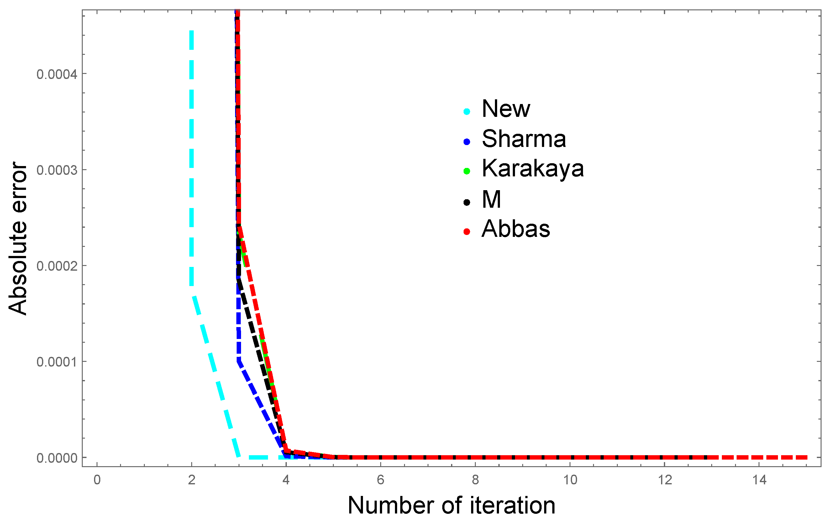
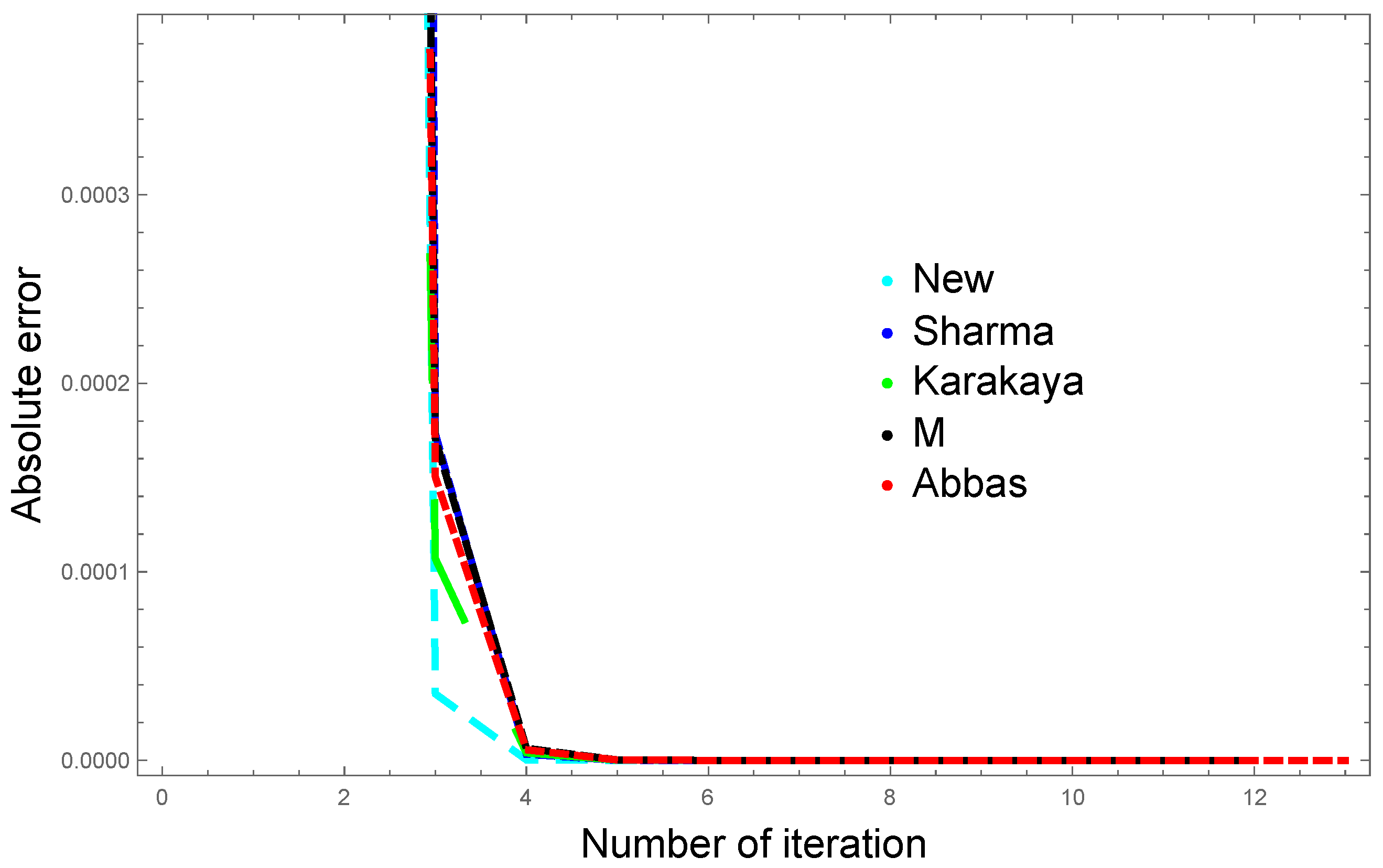
Since in the given examples the mapping $\Gamma$ satisfies the given contractive condition on a complete space, hence, we can also use our new iterative scheme to approximate the fixed points. We compare our results with the Sharma, Karakaya, M., and Abbas iterations for various choices of set of parameters and initial points using Table 1 and Table 2. The graphical analysis is provided in Figure 1 and Figure 2. Clearly, all the tables and graphs suggest that our new approach is highly accurate and gives effective accuracy in fewer iterations.

Table 1. Absolute error comparison of various iterative schemes for ${\sigma }_n={\displaystyle \frac{n+2}{\sqrt[3]{n+1}}}$, and $\mu =1.0$.

n	New	Sharma	Karakaya	M	Abbas
1	0.6178569153	0.6097295906	0.6283899067	0.6261605913	0.6287944212
2	0.0001770274	0.0082029991	0.0105834463	0.0083058168	0.0109966797
3	4.59584 (−8)	0.0001001622	0.0002341580	0.0001844357	0.0002431310
4	1.19311 (−11)	1.22158 (−6)	6.86816 (−6)	5.40926 (−6)	7.13147 (−6)
5	3.10862 (−15)	1.48984 (−8)	2.48667 (−7)	1.95847 (−7)	2.58200 (−7)
6	0.0000000000	1.81700 (−10)	1.06332 (−8)	8.37459 (−9)	1.10408 (−8)
7	0.0000000000	2.21600 (−12)	5.21333 (−10)	4.10595 (−10)	5.41319 (−10)
8	0.0000000000	2.70894 (−14)	2.86974 (−11)	2.26016 (−11)	2.97966 (−11)
9	0.0000000000	2.22044 (−16)	1.74638 (−12)	1.37512 (−12)	1.81366 (−12)
10	0.0000000000	0.0000000000	1.16573 (−13)	9.12603 (−14)	1.20792 (−13)

Table 2. Absolute error comparison of various iterative schemes for ${\sigma }_n=0.65$, and $\mu =0.6$.

n	New	Sharma	Karakaya	M	Abbas
1	0.4071498001	0.4017526881	0.0912785378	0.0930058087	0.0924390089
2	0.0043524550	0.0098843889	0.0028488193	0.0046373364	0.0040510574
3	0.0000352918	0.0001730132	0.0001068721	0.0001704100	0.0001502011
4	2.95231 (−7)	3.25208 (−6)	3.99034 (−6)	6.36753 (−6)	5.61060 (−6)
5	2.46912 (−9)	6.10544 (−8)	1.49016 (−7)	2.37784 (−7)	2.09520 (−7)
6	2.06500 (−11)	1.14625 (−9)	5.56487 (−9)	8.87982 (−9)	7.82433 (−9)
7	1.72528 (−13)	2.15203 (−11)	2.07814 (−10)	3.31608 (−10)	2.92191 (−10)
8	1.33226 (−15)	4.04121 (−13)	7.76079 (−12)	1.23835 (−11)	1.09116 (−11)
9	0.0000000000	7.77156 (−15)	2.89879 (−13)	4.62407 (−13)	4.07451 (−13)
10	0.0000000000	2.22044 (−16)	1.07691 (−14)	1.73194 (−14)	1.50990 (−14)

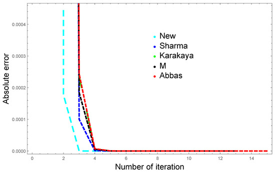
Figure 1. Graphical analysis of iterates.

Figure 2. Graphical analysis of iterates.

6. Application of $\mathbf{2}\mathit{D}$ Volterra Integral Equation

In recent years, the study of $2D$ Volterra equations has gained the attention of many authors (see, e.g., [40,41] and others). In this portion, we investigate how our main results can be applied to the nonlinear $2D$ Volterra integral equation of the form:

$$\begin{array}{ccc}\hfill \nu (\alpha ,\beta )& =& \kappa (\alpha ,\beta )+{\int }_0^{\alpha }{\int }_0^{\beta }{G}_1(g,h,\nu (g,h))\varrho g\varrho h+\varphi {\int }_0^{\alpha }{G}_2(\beta ,h,\nu (\alpha ,h))\varrho h\hfill \\ & & +\pi {\int }_0^{\beta }{G}_3(\alpha ,g,\nu (\beta ,g))\varrho g,\hfill \end{array}$$

(48)

for all $\alpha ,\beta ,g,h\in [0,1]$, where $\nu \in \Delta \times \Delta ,\kappa :[0,1]\times [0,1]\to {\mathbb{R}}^2,G_i(i=1,2,3):[0,1]\times [0,1]\times {\mathbb{R}}^2\to {\mathbb{R}}^2,\varphi ,\pi \ge 0$ and $\Delta =C\left(\right[0,1\left]\right)$ is a Banach Space with the maximum norm

$$\begin{array}{c}\hfill \left|\right|w-{v\left|\right|}_{\infty }=\underset{t\in [0,1]}{max}|w\left(t\right)-v\left(t\right)|,\end{array}$$

for all $w,v\in C\left(\right[0,1\left]\right)$.

We now suggest the following main result.

Theorem 6. 

Assume that we have a convex closed and nonempty subset $\mathfrak{D}$ of a given Banach space and Γ a selfmap of $\mathfrak{D}$ is defined by

$$\begin{array}{ccc}\hfill \Gamma \nu (\alpha ,\beta )& =& \kappa (\alpha ,\beta )+{\int }_0^{\alpha }{\int }_0^{\beta }{G}_1(g,h,\nu (g,h))\varrho g\varrho h+\varphi {\int }_0^{\alpha }{G}_2(\beta ,h,\nu (\alpha ,h))\varrho h\hfill \\ & & +\pi {\int }_0^{\beta }{G}_3(\alpha ,g,\nu (\beta ,g))\varrho g.\hfill \end{array}$$

Consider the following conditions:

($A_1$) 

The map $\nu :\mathfrak{B}\times \mathfrak{B}\to {\mathbb{R}}^2$ is essentially continuous.

($A_2$) 

The two maps $G_i(i=1,2,3):[0,1]\times [0,1]\times {\mathbb{R}}^2\to {\mathbb{R}}^2$ are also continuous such that one has constants $g_1,g_2,g_3>0$ with

$$\begin{array}{ccc}\hfill |G_1(g,h,w_1(g,h))-G_1(g,h,w_2(g,h))|& \le & g_1|w_1-w_2|,\hfill \\ \hfill |G_2(g,h,w_1(g,h))-G_2(g,h,w_2(g,h))|& \le & g_2|w_1-w_2|,\hfill \\ \hfill |G_3(g,h,w_1(g,h))-G_3(g,h,w_2(g,h))|& \le & g_3|w_1-w_2|,\hfill \end{array}$$

for $w_1,w_2\in {\mathbb{R}}^2$.

($A_3$) 

For $\varphi ,\pi \ge 0,g_1+\varphi g_2+\pi g_3=\rho$, where $\rho \in (0,1)$.

In this case, the $2D$ Volterra Integral Equation (48) and our new iteration converge to a solution.

Proof. 

For any $\nu ,{\nu }^{*}\in \mathfrak{B}\times \mathfrak{B}$, one has

$$\begin{array}{ccc}\hfill \left|\right|\nu -\Gamma {\nu }^{*}{\left|\right|}_{\infty }& =& \underset{t\in [0,1]}{max}|\nu (\alpha ,\beta )\left(t\right)-\Gamma {\nu }^{*}(\alpha ,\beta )|\hfill \\ & =& \underset{t\in [0,1]}{max}|\nu (\alpha ,\beta )\left(t\right)-\kappa (\alpha ,\beta )\left(t\right)-{\int }_0^{\alpha }{\int }_0^{\beta }{G}_1(g,h,{\nu }^{*}(g,h))\varrho g\varrho h\hfill \\ & & -\varphi {\int }_0^{\alpha }{G}_2(\beta ,h,{\nu }^{*}(\alpha ,h))\varrho h-\pi {\int }_0^{\beta }{G}_3(\alpha ,g,{\nu }^{*}(\beta ,g))\varrho g|\hfill \\ & \le & \underset{t\in [0,1]}{max}\left\{\right|\nu (\alpha ,\beta )\left(t\right)-\kappa (\alpha ,\beta )\left(t\right)-{\int }_0^{\alpha }{\int }_0^{\beta }{G}_1(g,h,\nu (g,h))\varrho g\varrho h\hfill \\ & & -\varphi {\int }_0^{\alpha }{G}_2(\beta ,h,\nu (\alpha ,h))\varrho h-\pi {\int }_0^{\beta }{G}_3(\alpha ,g,\nu (\beta ,g))\varrho g|\hfill \\ & & +|{\int }_0^{\alpha }{\int }_0^{\beta }{G}_1(g,h,\nu (g,h))\varrho g\varrho h-{\int }_0^{\alpha }{\int }_0^{\beta }{G}_1(g,h,{\nu }^{*}(g,h))\varrho g\varrho h|\hfill \\ & & +\varphi |{\int }_0^{\alpha }{G}_2(\beta ,h,\nu (\alpha ,h))\varrho h-{\int }_0^{\alpha }{G}_2(\beta ,h,{\nu }^{*}(\alpha ,h))\varrho h|\hfill \\ & & +\pi |{\int }_0^{\beta }{G}_3(\alpha ,g,{\nu }^{*}(\beta ,g))\varrho g-{\int }_0^{\beta }{G}_3(\alpha ,g,{\nu }^{*}(\beta ,g))\varrho g\left|\right\}\hfill \\ & \le & \underset{t\in [0,1]}{max}|\nu (\alpha ,\beta )\left(t\right)-\Gamma \nu (\alpha ,\beta )|+g_1\underset{t\in [0,1]}{max}{\int }_0^{\alpha }{\int }_0^{\beta }|\nu (g,h)\hfill \\ & & -{\nu }^{*}(g,h)|\varrho g\varrho h+\varphi g_2\underset{t\in [0,1]}{max}{\int }_0^{\alpha }|\nu (g,h)-{\nu }^{*}(g,h)|\varrho h\hfill \\ & & +\pi g_3\underset{t\in [0,1]}{max}{\int }_0^{\beta }|\nu (g,h)-{\nu }^{*}(g,h)|\varrho g,\hfill \end{array}$$

which implies that

$$\begin{array}{ccc}\hfill \left|\right|\nu -\Gamma {\nu }^{*}{\left|\right|}_{\infty }& \le & \underset{t\in [0,1]}{max}|\nu (\alpha ,\beta )\left(t\right)-\Gamma \nu (\alpha ,\beta )|+g_1\underset{t\in [0,1]}{max}|\nu (g,h)-{\nu }^{*}(g,h)|\hfill \\ & & +\varphi g_2\underset{t\in [0,1]}{max}|\nu (g,h)-{\nu }^{*}(g,h)|+\pi g_3\underset{t\in [0,1]}{max}|\nu (g,h)-{\nu }^{*}(g,h)|\hfill \\ & \le & \left|\right|\nu -\Gamma {\nu }^{*}{\left|\right|}_{\infty }+(g_1+\varphi g_2+\pi g_3)\underset{t\in [0,1]}{max}|\nu (g,h)-{\nu }^{*}(g,h)|\hfill \\ & \le & \left|\right|\nu -\Gamma {\nu }^{*}{\left|\right|}_{\infty }+\rho \left|\right|\nu -{\nu }^{*}{\left|\right|}_{\infty }.\hfill \end{array}$$

Hence, (11) is satisfied with $\rho =g_1+\varphi g_2+\pi g_3$, where $\rho \in (0,1)$ and so it follows that our fixed-point iteration converges to the solution. □

7. Conclusions and Future Plan of Work

In this paper, we provide the following new results:.

(i)

A new fixed-point iterative scheme for nonlinear problems in a Banach space setting is provided.

(ii)

The convergence result for the iterative scheme is proved under some mild conditions.

(iii)

Some qualitative results associated with stability, data dependency, and order are proven.

(iv)

Many new nonlinear problems are constructed, and it has been proven numerically that our new iteration converges faster to the solution as compared to the other iterative schemes.

(v)

An application of our new iterative scheme is provided for finding solutions to the 2D nonlinear Volterra Integral Equation (VIE).

(vi)

In the future, we will extend the presented results to the setting of multi-valued mappings and common fixed-point problems.

References

- Alakoya, T.O.; Mewomo, O.T. Viscosity S-iteration method with inertial technique and self-adaptive step size for split variational inclusion, equilibrium and fixed point problems. Comput. Appl. Math. 2022, 41, 39. [Google Scholar] [CrossRef]
- Alakoya, T.; Uzor, V.; Mewomo, O. A new projection and contraction method for solving split monotone variational inclusion, pseudomonotone variational inequality, and common fixed point problems. Comput. Appl. Math. 2022, 42, 3. [Google Scholar] [CrossRef]
- Alakoya, T.O.; Uzor, V.A.; Mewomo, O.T.; Yao, J.C. On a system of monotone variational inclusion problems with fixed point constraint. J. Inequal. Appl. 2022, 47, 47. [Google Scholar] [CrossRef]
- Uzor, V.A.; Alakoya, T.O.; Mewomo, O.T. On split monotone variational inclusion problem with multiple output sets with fixed point constraints. Comput. Methods Appl. Math. 2023, 23, 729–749. [Google Scholar] [CrossRef]
- Shatanawi, W.; Shatnawi, T.A.M. New fixed point results in controlled metric type spaces based on new contractive conditions. Aims Math. 2023, 8, 9314–9330. [Google Scholar] [CrossRef]
- Joshi, M.; Tomar, A.; Abdeljawad, T. On fixed points, their geometry and application to satellite web coupling problem in S-metric spaces. Aims Math. 2023, 8, 4407–4441. [Google Scholar] [CrossRef]
- Rezazgui, A.Z.; Tallafha, A.A.; Shatanawi, W. Common fixed point results via Av α-contractions with a pair and two pairs of self-mappings in the frame of an extended quasi b-metric space. Aims Math. 2023, 8, 7225–7241. [Google Scholar] [CrossRef]
- Browder, F.E. Nonexpansive nonlinear operators in Banach space. Proc. Natl. Acad. Sci. USA 1965, 54, 1041–1044. [Google Scholar] [CrossRef]
- Gohde, D. Zum Prinzip der Kontraktiven Abbildung. Math. Nachr. 1965, 30, 251–258. [Google Scholar] [CrossRef]
- Kirk, W.A. A fixed point theorem for mappings which do not increase distances. Am. Math. Mon. 1965, 72, 1004–1006. [Google Scholar] [CrossRef]
- Rhoades, B. Fixed point iterations for certain nonlinear mappings. J. Math. Anal. Appl. 1994, 183, 118–120. [Google Scholar] [CrossRef]
- Rhoades, B. Some theorems on weakly contractive maps. Nonlinear Anal. TMA 2001, 47, 2683–2693. [Google Scholar] [CrossRef]
- Suzuki, T. Fixed point theorems and convergence theorems for some generalized nonexpansive mapping. J. Math. Anal. Appl. 2008, 340, 1088–1095. [Google Scholar] [CrossRef]
- Mann, W.R. Mean value methods in iteration. Proc. Am. Math. Soc. 1953, 4, 506–510. [Google Scholar] [CrossRef]
- Ishikawa, S. Fixed points by a new iteration method. Proc. Am. Math. Soc. 1974, 44, 147–150. [Google Scholar] [CrossRef]
- Agarwal, R.; Regan, D.O.; Sahu, D. Iterative construction of fixed points of nearly asymptotically nonexpansive mappings. J. Nonlinear Convex Anal. 2007, 8, 61–79. [Google Scholar]
- Chugh, R.; Kumar, V.; Kumar, S. Strong convergence of a new three step iterative scheme in Banach spaces. Am. J. Comput. Math. 2012, 2, 345–357. [Google Scholar] [CrossRef]
- Gursoy, F.; Karakaya, V. A Picard-S hybrid type iteration method for solving a differential equation with retarded argument. arXiv 2014, arXiv:1403.2546. [Google Scholar]
- Hacioglu, E.; Gursoy, F.; Maldar, S.; Atalan, Y.; Milovanovic, G.V. Iterative approximation of fixed points and applications to two-point second order boundary value problems and to machine learning. Appl. Numer. Math. 2021, 167, 143–172. [Google Scholar] [CrossRef]
- Kanwar, V.; Sharma, P.; Argyros, I.K.; Behl, R.; Argyros, C.; Ahmadian, A.; Salimi, M. Geometrically constructed family of the simple fixed point iteration method. Mathematics 2021, 9, 694. [Google Scholar] [CrossRef]
- Karakaya, V.; Atalan, Y.; Dogan, K.; Bouzara, N.E.H. Some fixed point results for a new three steps iteration process in Banach spaces. Fixed Point Theory 2017, 18, 625–640. [Google Scholar] [CrossRef]
- Mebawondu, A.A.; Mewomo, O.T. Fixed point results for a new three steps iteration process. Ann. Univ. Craiova-Math. Comput. Sci. Ser. 2019, 46, 298–319. [Google Scholar]
- Ullah, K.; Arshad, M. Numerical reckoning fixed points for Suzuki’s generalized nonexpansive mappings via new iteration process. Filomat 2018, 32, 187–196. [Google Scholar] [CrossRef]
- Abbas, H.; Mebawondu, A.; Mewomo, O. Some results for a new three steps iteration scheme in Banach spaces. Bull. Transilv. Univ. Brasov. Math. Inform. Phys. Ser. III 2018, 11, 1–18. [Google Scholar]
- Abbas, M.; Nazir, T. A new faster iteration process applied to constrained minimization and feasibility problems. Math. Vesnik 2014, 66, 223–234. [Google Scholar]
- Noor, M.A. New approximation schemes for general variational inequalities. J. Math. Anal. Appl. 2000, 251, 217–229. [Google Scholar] [CrossRef]
- Phuengrattana, W.; Suantai, S. On the rate of convergence of Mann, Ishikawa, Noor and SP-iterations for continuous functions on an arbitrary interval. J. Comput.Appl. Math. 2011, 235, 3006–3014. [Google Scholar] [CrossRef]
- Sharma, P.; Ramos, H.; Behl, R.; Kanwar, V. A new three-step fixed point iteration scheme with strong convergence and applications. J. Comput. Appl. Math. 2023, 430, 115242. [Google Scholar] [CrossRef]
- Suantai, S. Weak and strong convergence criteria of Noor iterations for asymptotically nonexpansive mappings. J. Math. Anal. Appl. 2005, 311, 506–517. [Google Scholar] [CrossRef]
- Thakur, B.S.; Thakur, D.; Postolache, M. A new iterative scheme for approximating fixed points of nonexpansive mappings. Filomat 2016, 30, 2711–2720. [Google Scholar] [CrossRef]
- Thianwan, S. Common fixed points of new iterations for two asymptotically nonexpansive nonself-mapping in a Banach space. J. Comput. Appl. Math. 2009, 224, 688–695. [Google Scholar] [CrossRef]
- Zamfirescu, T. Fix point theorems in metric space. Arch. Math. 1972, 23, 292–298. [Google Scholar] [CrossRef]
- Berinde, V. Iterative Approximation of Fixed Points; Springer: Berlin/Heidelberg, Germany, 2007. [Google Scholar]
- Osilike, M. Stability results for fixed point iteration procedures. J. Nigerian Math. Soc. 1995, 14, 17–29. [Google Scholar]
- Imoru, C.O.; Olatinwo, M.O. On the stability of Picard and Mann iteration processes. Carpathian J. Math. 2003, 19, 155–160. [Google Scholar]
- Berinde, V. On the stability of some fixed point procedures. Bul. Stiint. Univ. Baia Mare Ser. B Mat.-Inform. 2002, 18, 7–14. [Google Scholar]
- Weng, X. Fixed point iteration for local strictly pseudo-contractive mapping. Proc. Am. Math. Soc. 1991, 113, 727–731. [Google Scholar]
- Harder, A.M. Fixed Point Theory and Stability Results for Fixed Point Iteration Procedures. Ph.D Thesis, University of Missouri, Rolla, MI, USA, 1987. [Google Scholar]
- Berinde, V. Picard iteration converges faster than Mann iteration for a class of quasi-contravtive operators. In Fixed Point Theory and Applications; Springer: Berlin/Heidelberg, Germany, 2004; Volume 2, pp. 1–9. [Google Scholar]
- Chauhan, H.V.S.; Singh, B.; Tunc, C.; Tunc, O. On the existence of solutions of non-linear 2D Volterra integral equations in a Banach Space. Rev. Real Acad. Cienc. Exactas Fis. Nat. Ser. A-Mat. 2022, 116, 101. [Google Scholar] [CrossRef]
- Deep, A.; Deepmala, T.C. On the existence of solutions of some non-linear functional integral equations in Banach algebra with applications. Arab. J. Basic Appl. Sci. 2020, 27, 279–286. [Google Scholar] [CrossRef]
Disclaimer/Publisher’s Note: The statements, opinions and data contained in all publications are solely those of the individual author(s) and contributor(s) and not of MDPI and/or the editor(s). MDPI and/or the editor(s) disclaim responsibility for any injury to people or property resulting from any ideas, methods, instructions or products referred to in the content. |
© 2024 by the authors. Licensee MDPI, Basel, Switzerland. This article is an open access article distributed under the terms and conditions of the Creative Commons Attribution (CC BY) license (https://creativecommons.org/licenses/by/4.0/).