Abstract
In this work, we present an up-scaling framework in a multi-scale setting to calibrate a stochastic material model. In particular with regard to application of the proposed method, we employ Bayesian updating to identify the probability distribution of continuum-based coarse-scale model parameters from fine-scale measurements, which is discrete and also inherently random (aleatory uncertainty) in nature. Owing to the completely dissimilar nature of models for the involved scales, the energy is used as the essential medium (i.e., the predictions of the coarse-scale model and measurements from the fine-scale model) of communication between them. This task is realized computationally using a generalized version of the Kalman filter, employing a functional approximation of the involved parameters. The approximations are obtained in a non-intrusive manner and are discussed in detail especially for the fine-scale measurements. The demonstrated numerical examples show the utility and generality of the presented approach in terms of obtaining calibrated coarse-scale models as reasonably accurate approximations of fine-scale ones and greater freedom to select widely different models on both scales, respectively.
1. Introduction
Randomness and heterogeneity are the main inherent characteristics that are found in almost all the materials that occur naturally or are engineered through man-made processes. Thus, the researchers/engineers—working in the relevant experimental and theoretical domains—have to take into account these characteristics while investigating a lab specimen or designing a structure made from the material under consideration. Specifically, in the context of computational mechanics, one of the most relevant problems is the characterization of micro-/meso-scale randomness and hence investigation of the effect of material heterogeneity on structural behavior through multi-scale numerical simulations. The previously mentioned approaches can be broadly classified into concurrent and non-concurrent approaches. Concurrent schemes consider both the coarse and fine scales during the course of the simulation, e.g., the FE-squared method [1,2], whereas the non-concurrent schemes are based on computing the desired Quantity of Interest (QoI) e.g., average stress, strain or energies, parameters for constitutive models, etc. through numerical experiments on a representative volume element (RVE) [3,4].
Focusing on the non-concurrent methods, there has been an increasing interest in incorporating material randomness aspects into computational studies. A classical approach in this regard is to perform numerical homogenization on an RVE ensemble that incorporates various sources of uncertainties—material properties, the spatial distribution of different phases and the size and shape of inclusions—and extract the relevant statistical QoI [5,6,7,8,9,10,11,12,13]. Moreover, extensive research in probabilistic numerics has yielded different numerical schemes to produce stochastic surrogate models for random microstructures with an aim to mitigate the effect of the curse of dimensionality due to the large number of sources of uncertainties encountered in such problems; see, e.g., [14,15,16,17]. Data-driven and machine learning-based approximate models, e.g., Neural Nets, have also been used in a similar pursuit [18,19,20,21,22,23]. The power of Deep Learning in Computational Homogenization has been leveraged in, e.g., [24,25,26,27,28] to yield a more elaborate fine-scale response in multi-scale computations. In recent times, the Physics-Informed Neural Networks (PINNs)—proposed in [29]—have gained huge popularity in the computational mechanics community. The main idea behind PINN is to incorporate physical principles, e.g., governing equations, boundary and initial conditions, etc., into the training phase of the neural network. In particular, with respect to the material calibration problem, both linear (elastic) [30,31,32] and non-linear (plasticity and damage) [33,34,35] problems have been explored. For accelerating multi-scale computations, the usage of PINN can be examined in [36,37,38]. Another interesting approach, based on unsupervised learning, has been devised in [39,40]. This approach automatically decides which computed material parameters (from a pool of constitutive models) are most relevant to the input measurements (e.g., displacements, strains, etc). It has been used for both elastic [40] and inelastic [41,42] model calibration. The utility of this approach in a probabilistic setting has been demonstrated in [43]. Furthermore, the methods based on Bayesian inference (which also forms the conceptual basis of our numerical scheme), to obtain a probabilistic description of coarse-scale characteristics through the incorporation of fine-scale measurements, have also been demonstrated in [44,45,46]. Bayesian methods allow for the explicit incorporation of uncertainty at both the fine scale (meso-scale) and the coarse scale (macro-scale). This is particularly important in up-scaling because material properties are often not deterministic but are influenced by variability in microstructure (e.g., distribution of inclusions, porosity). By considering both epistemic uncertainty (knowledge uncertainty) and aleatory uncertainty (inherent randomness), Bayesian methods provide a more complete understanding of material behavior, including confidence intervals for predictions. Unlike traditional methods, which typically provide point estimates (e.g., the mean value properties like in the classical homogenization), Bayesian up-scaling produces a probabilistic distribution of the coarse-scale material properties.
In this paper, we demonstrate the application of the Bayesian up-scaling framework developed in [47,48] for the computational homogenization of concrete. The detailed structure of concrete at the meso-scale is studied, including the arrangement and behavior of its components. This information is then translated to the macro-scale, where the focus shifts to the overall material performance. The homogenization process converts these detailed properties into more manageable parameters that can be used to predict concrete’s behavior in real-world engineering applications. When framed within a Bayesian context, computational homogenization not only provides predictions of macro-scale material properties but also quantifies the confidence or epistemic uncertainty in these predictions. It offers an automatic homogenization procedure, as described in [47,48], using a deterministic representative volume element as an example. Taking this a step further, this paper addresses a more general case in which the meso-scale description also varies. Specifically, we account for aleatory uncertainty that represents the geometric arrangement of aggregates within the matrix phase. To extend the Bayesian up-scaling procedure, we apply it to the homogenization of a stochastic representative volume element. We model the meso-scale concrete using a fine-tuned stochastic finite element model, which describes the behavior of an ensemble of representative volume elements with a random distribution of inclusions in the matrix phase. At the macro-scale, the material behavior is represented by a super-element, or coarse scale, which accounts for the homogeneous material properties obtained through the Bayesian up-scaling procedure. Due to the aleatory uncertainty at the meso-scale (referred to as the fine scale), the coarse-scale representation also becomes stochastic. This includes both epistemic uncertainty introduced by the Bayesian up-scaling algorithm and the aleatory uncertainty arising from variations at the meso-scale.
Thus, the goal is to estimate the continuous distribution of the coarse scale properties given the discrete version (samples) of stochastic fine scale measurements. The novelty of this work stems from two new advancements. Firstly, the numerical finite element (FE) schemes employed to model concrete material behavior on both the scales differ completely with respect to the elements they use: namely, the material specimen on the coarse scale uses continuum elements, whereas the fine scale is composed of discrete truss elements to approximate the solution field. This example scenario highlights the generality of the up-scaling scheme in terms of its applicability. Secondly, we propose the unsupervised learning method for the estimation of the stochastic coarse-scale properties. This method is based on the approximate Bayesian estimation with the help of the generalized Kalman filter based on the polynomial chaos approximation as proposed in [49]. As this method requires the functional approximation of the fine-scale measurements, one has to be able to evaluate the polynomial chaos approximation of the fine-scale measurement by using standard uncertainty quantification techniques. Having in mind that the fine scale representation depends on many parameters used to describe the detailed heterogeneous material properties, such an approach is usually practically not feasible. Therefore, we suggest using an unsupervised learning technique for the fine-scale parameter reduction. In other words, we utilize the transport maps approach [50,51,52] to transform the fine-scale measurement samples from the high-dimensional nonlinear space to low-dimensional Gaussian space. Once the minimal parameterization is found, one may construct the required functional approximation of fine-scale measurement, therefore avoiding the complications related to constructing measurement approximation from a high-dimensional stochastic process, generating fine-scale material realizations and the need to incorporate significant modifications in the already existing up-scaling framework.
The contents in the paper are presented as follows: Section 2 describes the abstract formulation of the up-scaling problem. Section 3 dwells briefly on the Bayesian framework, stating the main results and the update formula for up-scaling. Section 4 presents the details on the computational scheme—with a major focus on constructing a functional approximation of fine-scale measurement—to be employed for conducting numerical experiments. Finally, in Section 5, examples illustrating the use of the up-scaling scheme are presented, and Section 6 concludes the discussion.
2. Abstract Formulation of Up-Scaling Problem
We consider a mechanical multi-scale problem composed of coarse and fine scales with an objective to calibrate the material characteristics of the former using the measurements from the latter. On the coarse scale, one considers an abstract model construct given as , which represents a rate-independent small-strain homogeneous macro-model in which denotes the state space, is a time-dependent energy functional, and is a convex and lower-semicontinuous dissipation potential satisfying and the homogeneity property for all . Then, in an abstract manner, the coarse-scale mechanical system can be described mathematically by the sub-differential inclusion
where stands for the Gâteux partial differential with respect to the state variable , and the derivative of is given in terms of the set-valued sub-differential in the sense of the convex analysis; see [53]. Moreover, the parameter vector represents the spatially homogeneous material characteristics governing the material behavior. On the fine scale, in terms of the formalism of stored energy and dissipation potential, one considers conceptually a similar model as the one on the coarse scale:
However, this model has a more elaborate description, encoded in its parameter , and it represents the material and geometrical/spatial variability of material properties on the fine scale. Such a material description lends itself to a higher computational cost when employed in a numerical scheme.
The numerical experiment consists of a material specimen under appropriate loading conditions. Keeping the same boundary conditions on the coarse and fine scales (and that the numerical schemes—employing the coarse and fine material models, respectively—are employed on the same specimen), the objective is to calibrate the coarse-scale to mimic a fine-scale model response as accurately as possible. Since , the states and cannot be directly compared as we will witness in the numerical illustration later in Section 5, where coarse- and fine-scale computational models are based on continuum and discrete truss elements, respectively, and the two models can only communicate in terms of some observables or measurements (e.g., energy, stress or strain, etc.) , where is typically some vector space like . In other words, one defines a measurement vector—obtained by the application of a respective measurement operator on the solution states—associated with the respective fine and coarse-scale models:
where and are the external excitation on the coarse and fine levels of similar type (i.e., either deformation or forced based), which are applied on the specimen boundaries. and are representing the corresponding abstract measurement operator on the prospective scales, whereas depicts the measurement noise associated with the fine scale. To draw parallels between the measurement output of the two models, one has to associate a random variable with the measurement . Here, is the triplet describing the probability space consisting of the set of all events, the sigma-algebra and the probability measure, respectively. represents the prediction of the measurement and modeling error that reflects the inability of the coarse-scale computational model to simulate the true/fine-scale measurement, or in other words represent the knowledge about . In this case, we assume that the modeling error is additive and model it a priori as a Gaussian distribution, the parameters of which are also learned during the up-scaling process. The stochastic version of , after the addition of , reads as
Since the objective of our study is to up-scale an ensemble of fine-scale material realizations, we introduce an additional type of uncertainty in our fine-scale material description which stems from an inherent randomness of the material. Considering the probabilistic view on such uncertainty, we model as a random variable/field in defined by mapping
Here, is the parameter space which depends on the application. Consequently, the evolution problem described by also becomes uncertain, so therefore Equation (2) is reformulated as
respectively. Once the uncertainty is present in the fine-scale model, the observation in Equation (3) modifies as
Following the previous formulation, the main goal is to estimate the distribution of the coarse-scale parameter given the set of discrete measurements of . To achieve this, we employ the Bayesian approach as described in the following section.
3. Bayesian Formulation of Stochastic Up-Scaling
The fine-scale material model characterized by a stochastic parameter vector renders the measurement in Equation (8) to be a random variable. This measurement should match the coarse-scale measurement in Equation (3) by tuning the corresponding unknown parameter . Thus, we would like to update by incorporating the information from the fine-scale measurement and hence obtain an indication on what the probability distribution for should be. To realize this, is assumed to be uncertain (unknown) and further modeled a priori as a random variable —prior—belonging to . Hence, the coarse-scale model in Equation (1) is converted into a stochastic one:
and subsequently a priori prediction of the coarse-scale measurement becomes
with . The goal is to identify the vector given using Bayes’s rule such that
holds. Here, is referred to as the posterior distribution of , as it incorporates the information from the fine-scale measurements via likelihood function , and is the normalization factor or evidence. Obtaining an analytical expression for is possible only in ideal cases, e.g., when both the prior and the likelihood are conjugate; i.e., they belong to the exponential family of distributions with predefined statistics. However, in most practical cases, obtaining full posterior is analytically intractable; hence, one has to resort to methods that are computationally expensive either due to evidence estimation or due to slow convergence of the random walk algorithms [54]. In the subsequent discussion, instead of focusing on obtaining the complete posterior information encoded in , we devise the algorithm to estimate posterior functional of in terms of a conditional expectation.
One last step, before we proceed to the next section, is to consider as the objective random variable for calibration, as is positive definite and this constraint has to be taken into consideration. In this way, computationally, whatever approximations or linear operations are performed on the numerical representation of , eventually taking is always going to be positive. Therefore, from this point onwards, we will use in developing Bayesian scheme for up-scaling.
Bayes Filter Using Conditional Expectation
The conditional expectation of with respect to the posterior distribution is given as
Instead of direct integration over the posterior measure, the conditional expectation can be estimated in a straightforward manner by projecting the random variable onto the subspace generated by the sub-sigma algebra of fine-scale measurement. To achieve this, one has to compute the minimal distance of to the point which can be defined in different ways. As shown by [49,55], the notion of distance can be generalized given a strictly convex, differentiable function with the hyperplane tangent to at point , such that
holds. Here, denotes the distance term that is also known as the Bregman’s loss function (BLF) or divergence. In general, the projection in Equation (13) is of a non-orthogonal kind and reflects the Bergman Pythagorean inequality:
that also holds for any arbitrary -measurable random variable . In case when , the previous relation rewrites to
in which the distance has a notion of variance, which is further referred to as Bregman’s variance. In terms of convex function , Bregman’s variance obtains the following form
For computational purposes, Bregman’s distance in Equation (13) is further taken as the squared Euclidean distance by assuming , such that and
In this case, Equation (14) reduces to the classical Pythagorean theorem. Moreover, one can show that the conditional expectation is the minimizer of the mean squared error and is the minimum variance unbiased estimator; kindly refer to [55] for detailed proof.
Focusing now on Equation (17), one may decompose the random variable belonging to into projected and residual components such that
holds. Here, is the orthogonal projection of the random variable onto the space of all distributions consistent with the data, whereas is its orthogonal residual. To give Equation (18) a more practical form, the projection term is further described by a measurable mapping according to the Doob–Dynkin lemma, which states
As a result, Equation (18) rewrites to
in which the first term in the sum, i.e., , is taken to be the projection of onto the fine-scale data set according to Equations (18) and (19), whereas is the residual component defined by a priori knowledge on the coarse scale. Following this, Equation (20) recasts to the update equation for the random variable as
in which is the assimilated random variable and is the observation prediction on the coarse scale given the prior . Therefore, to estimate , one requires only information on the map . For the sake of computational simplicity, the map in Equation (19) is further approximated in a Galerkin manner by a family of polynomials
such that the filter in Equation (21) rewrites to
As the map in Equation (22) is parameterized by a set of coefficients , i.e., , these further can be found by minimizing the residual component (the optimality condition in Equation (17)):
In an affine case, when , the previous optimisation outcomes in a formula defining the well-known Kalman gain:
such that the update formula in Equation (23) reduces to the generalization of the Kalman filter
which is here referred as a Gauss–Markov–Kalman filter; for more details, please see [56].
4. Computational Scheme for Up-Scaling
The update Equation (26) derived in the previous section needs to be realized in a computational framework to illustrate the use of the up-scaling scheme. In concrete terms, one requires a numerical approximation of the involved random variables in Equation (23). A widely used strategy in this regard is to use an ensemble of sampling points for the random material parameters of coarse and fine-scale models, which leads to an ensemble-based interpretation of Kalman filter (EnKF). We pursue a different path here to discretize the RVs in Equation (26), and a functional approximation is employed; i.e., the RVs are defined in terms of functions of known standard RVs. We shall assume that these have been chosen to be independent and often even normalized Gaussians. The final step in describing the computational versions of RVs in Equation (26) is to choose a finite set of linearly independent functions of these base RVs, where the index represents a multi-index, and the set of multi-indices for approximation is a finite set with cardinality (size) Z. There are several systems of functions that can possibly be used in this regard, e.g., polynomial chaos expansion (PCE) or generalized PCE (gPCE) [57], kernel functions [58], radial basis functions [59], or functions derived from a fuzzy set [60]. In this work, all the subsequent development is carried out in terms of PCE-based approximation. In the following discussion, we describe the computational procedure to develop the PCE approximation for coarse and fine scales. Moreover, it merits mentioning here that the PCE for all the relevant RVs are computed in a non-intrusive fashion (details of the related methods are out of the scope of this paper; the interested reader can consult [49,61,62,63,64] for more information), meaning the PCE approximations are computed using samples, i.e., the material parameters are sampled from their associated probability density functions (PDFs), and the corresponding energy measurements are obtained by repeated execution of the deterministic FEM solvers for coarse and fine scales, respectively.
4.1. Coarse-Scale Prior and Energy Approximation
The PCE approximation of coarse-scale prior material properties modeled as log-normal RVs to preserve the positive-definitiveness property, , see Equation (10), can be easily constructed by using the basis defined in terms of standard normal RVs that are sampled according to . These random variables are known, as they are constructed by experts. Having at hand, the material samples are obtained from it using the seed from . These material samples are then fed into the FEM computational model to obtain for each sample the solution field (see Equation (10)) and the corresponding prediction of the energy measurement using the measurement operator ; see Equation (11). Consequently, one can obtain the PCE approximation for energy as , where L is the number of different types of predicted energy measurements (e.g., stored energy, dissipation, etc). The procedure to construct predicted energy PCE is summarized in Algorithm 1.
| Algorithm 1 Coarse-scale energy PCE |
|
4.2. Fine-Scale Measurement Approximation
The up-scaling scheme presented in this paper deals with a stochastic fine-scale material model; therefore, the resulting measurement in Equation (9)—to be used to update the coarse-scale material model—reflects the inherent randomness (aleatoric uncertainty) of the fine scale. This scenario poses a hurdle to construct the fine-scale measurement PCE approximation mainly due to two reasons:
- The underlying process to generate the fine-scale material realizations is not available; i.e., we do not have the continuous data (in a form of a random variable). Rather, we have its discrete version given as a set of random fine-scale realizations (e.g., from real experiments).
- Even if the random process—generating the fine-scale realizations—is available, e.g., in a computational setting (as in the numerical experiments of Section 5), computing the corresponding energy PCE is not easily achievable. This is due to the high-dimensional and spatially varying nature of the fine-scale material description (e.g., properties described by a random field or the random distribution of different material phases), resulting in a more involved and computationally expensive procedure due to the large number of unknown PCE coefficients.
To tackle this problem, the idea is to model the fine-scale response as a nonlinear mapping of some basic standard random variable such that
holds. The random variable is not known a priori and is to be determined. Similarly, the map in Equation (28) is parameterized by coefficient vector , which also needs to be determined. Therefore, the problem boils down to estimating , which is solved in two steps. We first transform samples to their standard normal counterparts . Secondly, using pairs, the parameters of the measurement map in Equation (28) are computed. This procedure—implemented using transport maps [51]—is detailed in the following discussion.
4.2.1. Transport Maps: Formal Definition
A transport map involves mapping a given (reference) random variable into another (target) random variable such that the probability measure of the target and the reference random variables is conserved. The idea was originally proposed by Monge [65] who formulated the problem of transporting a unit mass associated with variable to another variable in terms of the following cost function
subjected to the constraint , where and are the probability measures of the respective RVs and is the pushforward operator. The result of the above problem is the transport map T, which is optimal in terms of incurring the lowest transportation cost. Transport maps have a wide domain of applications in various fields [66,67,68,69,70,71,72,73,74,75,76].
To construct the transport map using the fine-scale energy samples , we use the approach that was first presented in [51] and discussed further in related research articles [50,52,77,78]. The method described here is adopted from [51], where it was originally proposed.
To put forth the problem in the current setting, we have at our disposal fine-scale energy samples: obtained from the corresponding FEM solver of the fine-scale model using input material property realizations ; see Equation (7). We seek to build an approximate map that transports energy samples of the target random variable—having PDF and measure —to the reference random variable samples having—PDF and measure . Furthermore, instead of seeking an optimal map by minimizing the cost function similar to Equation (29), we explicitly specify the sought map to have a Lower Triangular structure that approximately satisfies the measure constraint , which is given as
The map is assumed to be monotone and is assumed to be differentiable. The induced density is given as
where and are the Jacobian and its absolute value calculated with respect to . In order to enforce the constraint exactly, the map-induced density should be equal to the exact one . Here, Kullback–Leibler (KL) divergence is used as a measure of discrepancy:
The above equation serves as an objective function that needs to be minimized. By slight reformulation, one arrives to
where is some space of lower-triangular functions in which we seek . We can further write the objective function in Equation (33) in form of a Monte Carlo approximation using the given fine-energy samples as
The discrete objective in Equation (34) still needs further modifications before it can be utilized in a practical optimization routine. For the sake of brevity, we briefly enumerate the necessary approximations concluded by the final optimization objective and some important remarks related to it.
- Specification of reference The reference random variable is taken as standard normal (as we aim to build the inverse map, i.e., a PCE approximation of fine-scale energy in terms of Hermite basis). The log of can be written as
- Separability of objective function: The lower triangular structure of the map renders the objective function to be split into L separate optimization problems (L being the dimensionality of the map). Hence, one can solve for each component of the map independently, where .
- Map parameterization: The last essential in solving the optimization problem is to approximate the map over some finite dimensional space which requires each component of the map to be parameterized in terms of some parameter set , hence assuming the form . This parameter set depends on the basis functions used to approximate the map, e.g., multivariate polynomials from a family of orthogonal polynomials or radial basis functions. After parameterization, the map is now defined in terms of container in which each element is a set containing the coefficients of the basis functions of the respective map component.
The final optimization problem after employing the above-mentioned modifications appears as
which has to be solved for parameter vector . The objective function in Equation (36) can be split into l separate problems (i.e., each component of map ), which are convex, linear in the respective parameter set and can be solved independently using Newton-based optimization algorithms [79].
4.2.2. PCE Approximation of Energy
In the discussion before, we have described the construction of a transport map using energy samples to obtain the corresponding output samples that are of standard normal type. Our aim is to construct a fine-scale measurement map in Equation (28) as a PCE approximation . In other terms, is the inverse of the originally computed transport map . Therefore, given the energy samples and their transformed standard counterparts, , such that , one may compute PCE for fine-scale energy measurement as
Compared to Equation (28), the parameters can be interpreted as the PCE coefficients of the chosen Hermite basis. The computation of fine-scale PCE is summarized in the Algorithm 2.
| Algorithm 2 Fine-Scale Energy PCE |
|
4.3. Coarse-Scale Parameter Estimation
Having the PCE approximations for coarse-scale prior , its energy prediction in Equation (27) and the fine-scale energy measurement in Equation (38); the corresponding up-scaled posterior is obtained by substituting the respective approximations into Equation (26). The resulting computational form of the update formula in Equation (26) appears in terms of PCE coefficients as
where denotes the coefficients of updated coarse-scale parameters PCE having fine-scale measurement information assimilated into them. is the well-known Kalman gain defined as
and evaluated directly from the prior PCE coefficients. In particular, the formula for covariance matrix reads
and analogously can be defined for other covariance matrices appearing in Equation (40).
The overall up-scaling procedure is further introduced in Algorithm 3.
| Algorithm 3 Up-Scaling |
|
5. Numerical Examples
In this section, we present the application of the proposed approach for the up-scaling methodology presented in the previous sections. The problem considered here is the estimation of coarse-scale homogeneous isotropic elastic phenomenological model parameters modeled on bi-phased concrete as random variables. The measurements come from a more elaborate fine-scale model whose stochastic nature is attributed to the random distribution of hard inclusions embedded in the soft matrix phase. In the following discussion, the computational setup for the modeling and simulation of coarse and fine-scale models is described, concluding with the presentation and the discussion of the results of the considered numerical experiment.
5.1. Computational Setup
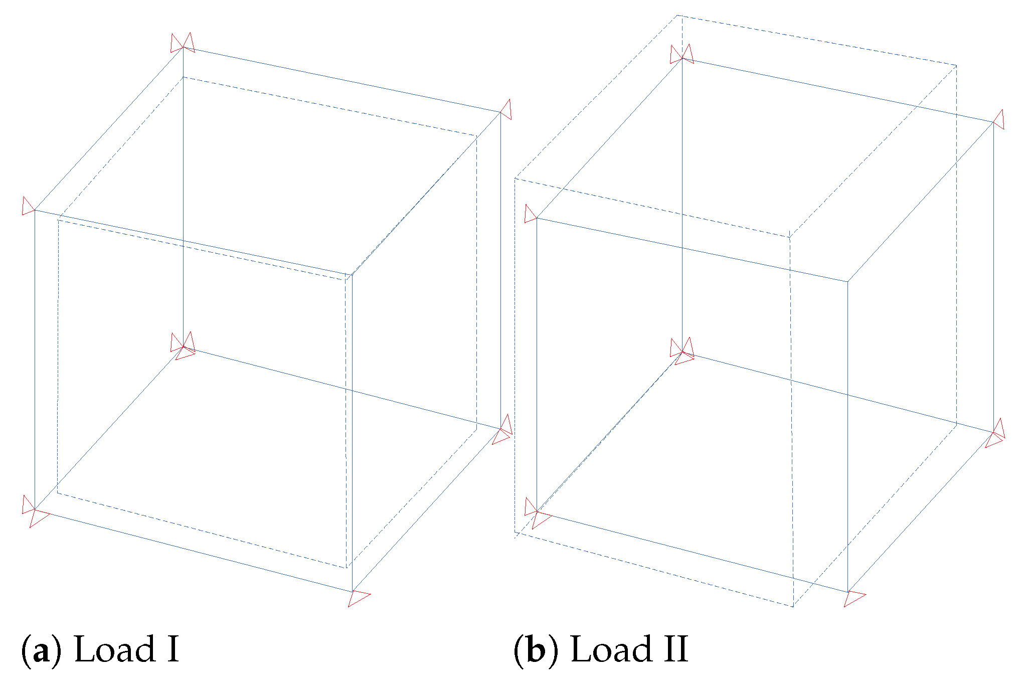
The material specimen is modeled as a 3D block of dimensions in cm. In order to extract the desired coarse-scale parameters, two displacement-based loading cases are considered: hydro-static compression as load case I and bi-axial tension–compression (pure shear) as load case II, the corresponding deformation tensor for the application of required displacement boundary conditions on the specimen faces is given as
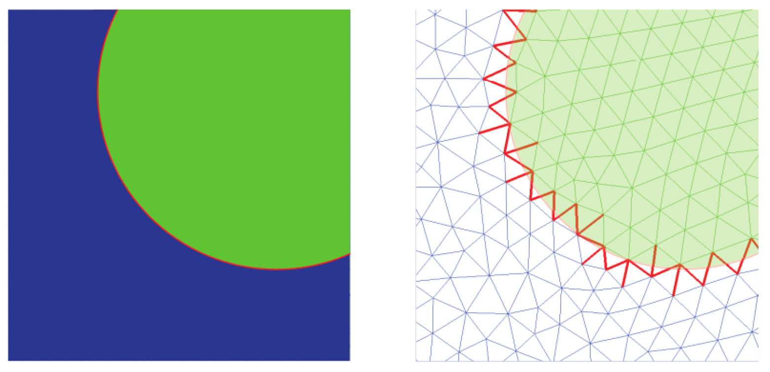
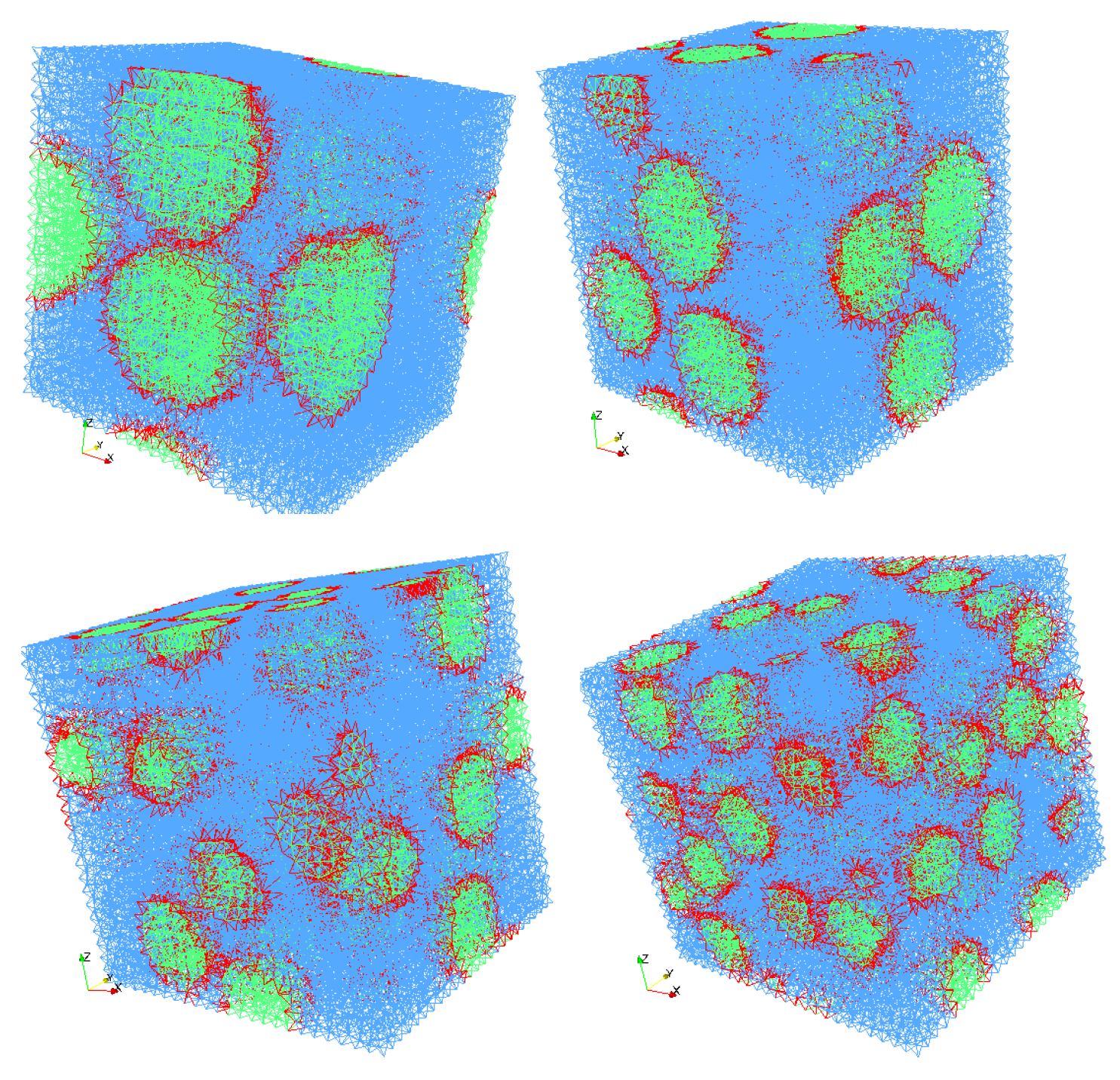
where p is the proportional factor taken as for the single load increment. The resulting deformations are illustrated in Figure 1. The specimen block is modeled as one 3D elastic brick element on the coarse scale with, i.e., as random parameters that need to be updated. As mentioned earlier, the fine-scale block comprises a random distribution of spherical inclusions in the matrix phase and is computationally represented by a lattice truss model. The adopted truss model has been proposed in [80] to model bi-phased material [81,82] (e.g., concrete) with an enhanced ability to model the interface between inclusion and the matrix phase (Figure 2 shows the deformation approximation of the two-phase material in the truss element). As a consequence, one does not need to explicitly model the interface, hence eliminating the need to employ a different mesh for each fine-scale realization, as illustrated graphically in Figure 3. This offers a great advantage of reduced computational burden in terms of mesh generation and also avoiding the mesh-related error variations when one considers an ensemble of fine-scale realizations. The truss elements are basically the edges of the tetrahedral elements filling the 3D block; the cross-section area of each element is obtained by the dual Voronoi tesselation of the tetrahedral mesh. Further details on the mesh generation and FE formulation of truss elements can be found in [82]. For the numerical examples considered here, the discrete fine-scale is composed of 58,749 truss elements (different realizations are shown in Figure 4).
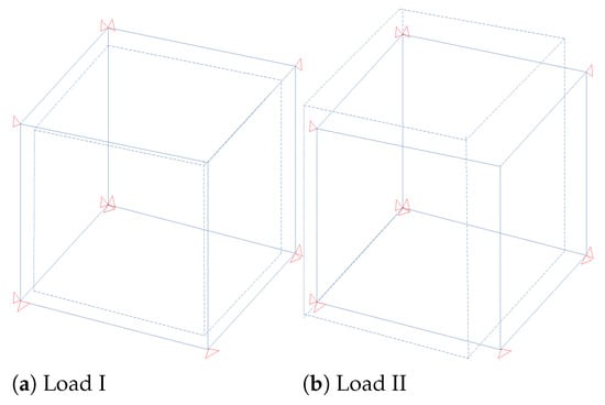
Figure 1.
Loading cases: (Load I) hydrostatic compression, (Load II) bi-axial tension–compression.
Figure 2.
Deformation approximation for the two-phase material in the truss element [82].
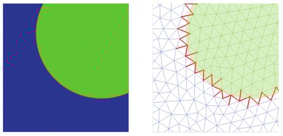
Figure 3.
Inclusion and matrix interface (left) and its FEM discretization with interface elements shown in red (right) [80].
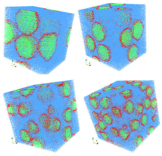
Figure 4.
Fine-scale realizations for different numbers of particles: embedded in the matrix phase.
The material parameters for inclusion and matrix phases, i.e., the Young modulli of their representative truss elements, are given in Table 1. For the interface element, an added parameter —which defines the relative proportion of inclusion and matrix phases in the element—is also computed and provided as input for the FE model.

Table 1.
Young modulli for fine-scale particle and matrix truss elements (in GPa).
The computational model for the fine scale is implemented as a User-Defined Element in the FEAP (Finite Element Analysis Program) Version 8.5 [83], which is a multi-purpose finite element program from University of California, Berkeley, CA, USA. Moreover, the computation of PCE approximations for material parameters and measurements and the update step in the Algorithm 3 (Section 4.3) of the up-scaling scheme are implemented in Matlab R2022b [84].
5.2. Verification Case: Up-Scaling One Fine-Scale Realization
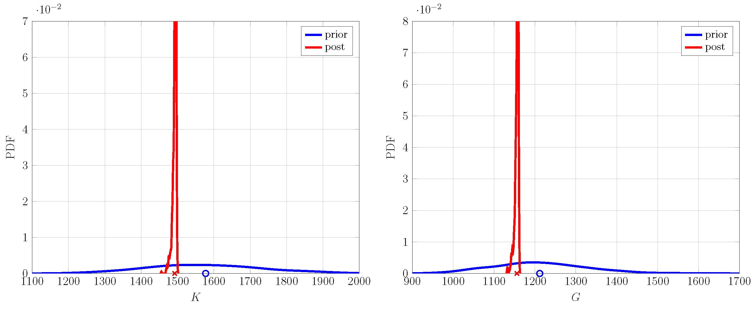
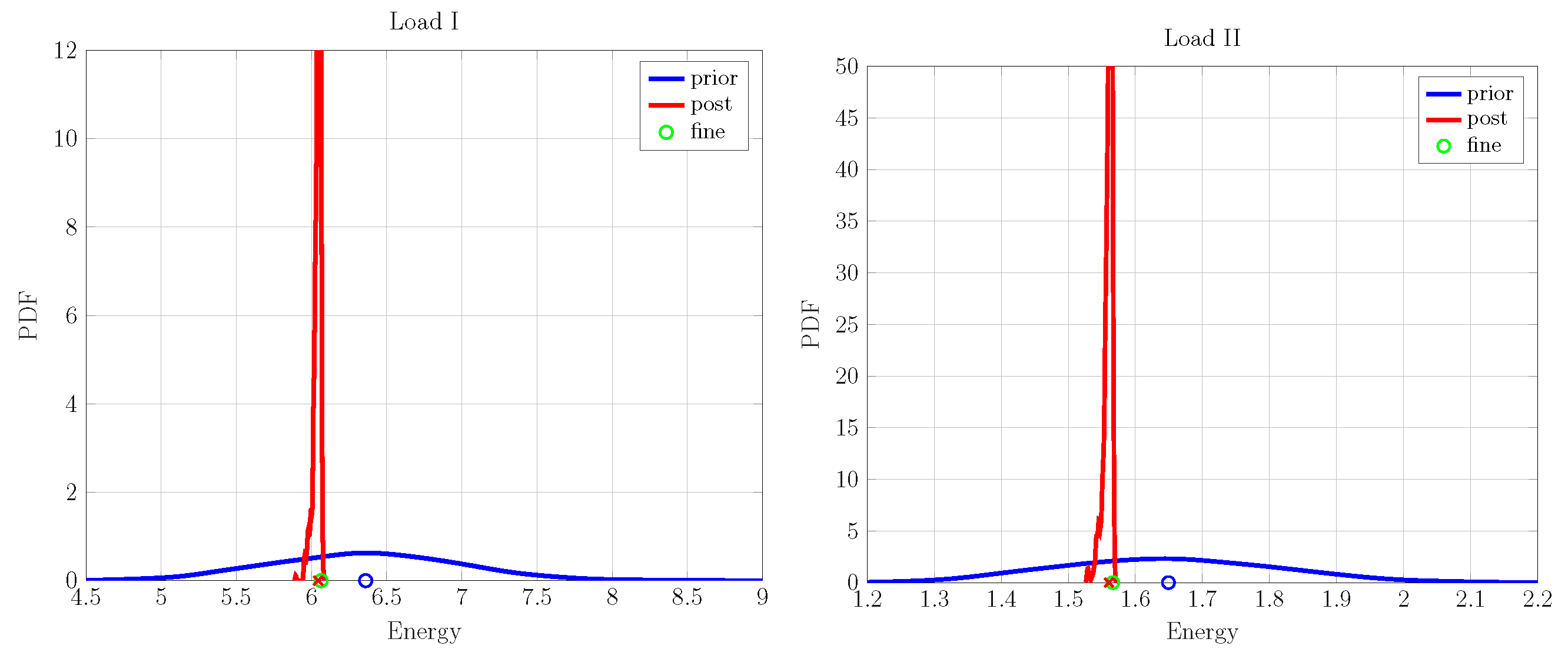
In this case, we demonstrate the working of an up-scaling framework on one fine-scale realization of a lattice model described previously. It is composed of 50 inclusions and a volume fraction. The prior characteristics of coarse-scale parameters are given in Table 2, and their corresponding probability density functions (PDFs) are shown in Figure 5 as prior distributions. The prior material properties are set as an input into the FEM simulation model to obtain the corresponding energies for the two loading cases; see Figure 1. The prior energy PDFs along—with their mean—are shown in Figure 6 in blue. The lack of knowledge regarding fine-scale characteristics on the coarse scale are reflected in the spread of energy PDFs and the offset of the mean values from the fine-scale counterpart. The PDF of posterior material properties (also shown in Figure 5)—after performing the up-scaling procedure—shows a marked reduction in their spread compared to the ones for prior properties. A similar behavior is observed in the posterior coarse-scale energy PDF, as shown in Figure 6. The uncertainty in the energy prediction of posterior properties is significantly reduced, and their respective mean values have shifted close to the fine-scale energy values, showing a negligible difference between the two values. Following this result, one may conclude that the Bayesian type of approach can be used to identify the properties of the coarse-scale continuum model given the fine-scale discrete measurement data.
Table 2.
Prior statistics in terms of mean and standard deviation values for coarse-scale material parameters (in MPa).
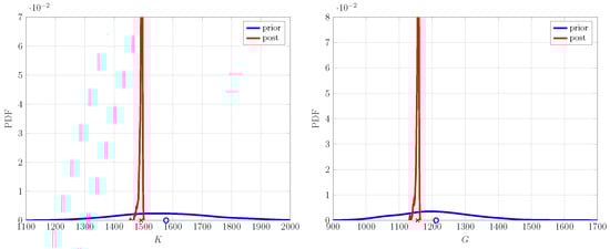
Figure 5.
Prior and posterior PDF for bulk K and shear G moduli on coarse-scale model, using one fine-scale realization.
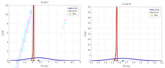
Figure 6.
Coarse-scale prior and posterior predicted energy PDFs for load cases: (I,II), using one fine-scale realization.
5.3. Up-Scaling Ensemble of Fine-Scale Realizations
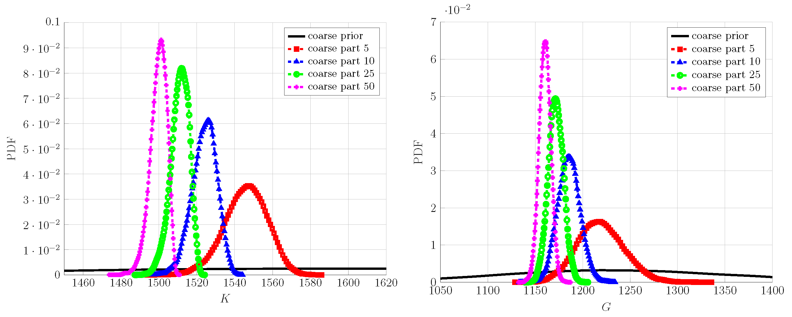
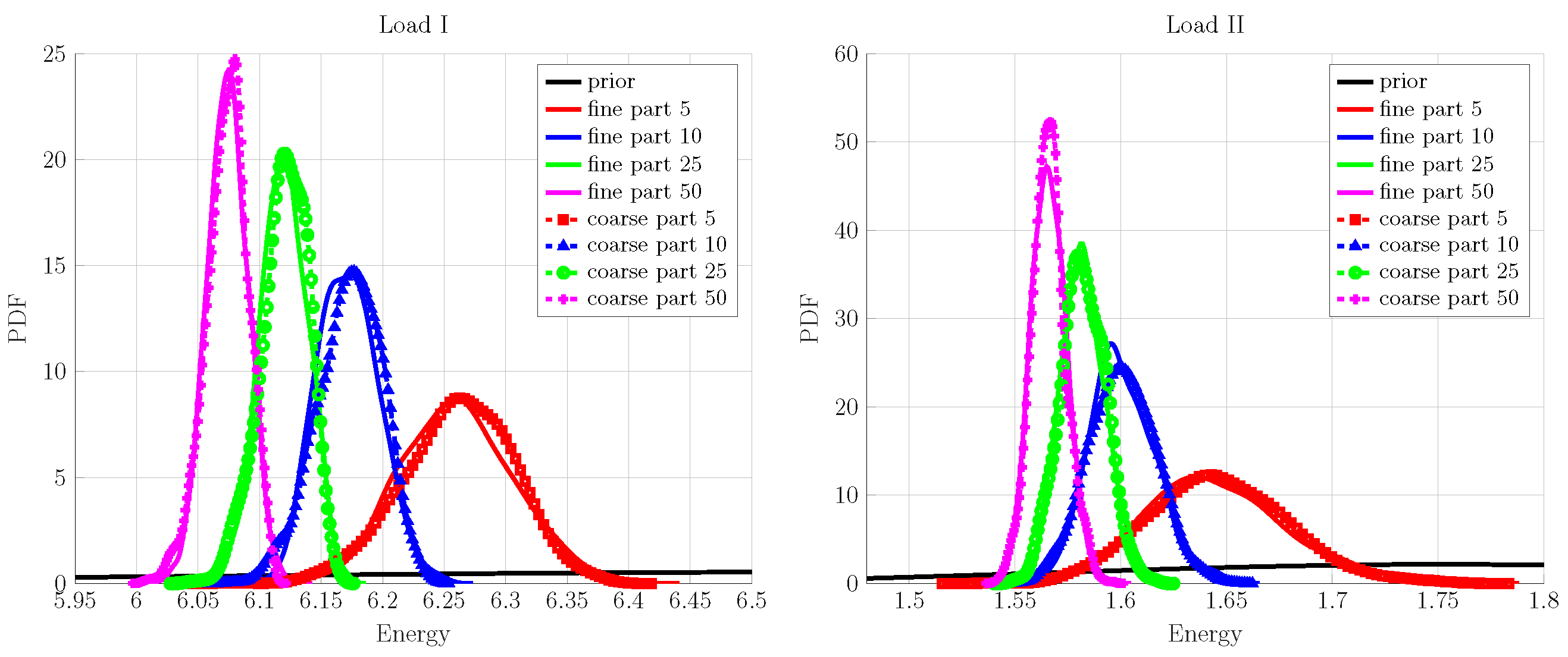
In this example, we consider a more realistic scenario of up-scaling an ensemble of fine-scale realizations. The main problem in this case is to construct the PCE approximations for the measured fine-scale energies. For this purpose, an ensemble of 1000 fine-scale realizations is generated for different numbers of particles: for a fixed volume fraction of 25%. The samples differ from one another by the placement of spherical inclusions using the Random Sequential Adsorption Algorithm [85] in the matrix phase. The corresponding ensemble of fine-scale energies is obtained by the discrete truss FEM model (described briefly in Section 5.1) for the two loading cases. The energy samples are then used to construct the transport map in order to obtain the corresponding standard normal samples; see Section 4.2.1. Having energy and its transformed value pairs at hand, the required PCE in Equation (37) approximation is constructed for fine-scale energy (detailed in Section 4.2). We have used the TransportMaps library [86] for map construction; in our example problem, the map is chosen to be of Isotropic Integrated Squared Triangular form and is parameterized using hermite polynomials (further details related to map types and related solvers for optimization problems can be found in the online help of the mentioned library). The PDF values of the measured fine-scale energies for the loading cases, presented in Figure 1, are shown in Figure 7, which shows that the inherent uncertainty of the fine scale is inversely proportional to the number of inclusions in the specimen. The largest spread is observed in the measurement PDF for specimen having five particles, whereas the 50 inclusions case represents the smallest variability, as expected. To estimate the bulk and shear moduli on the coarse scale, we need to make an assumption on the prior uncertainty. Based on the homogenization theory [87], each sample of fine-scale realization of the fine energy measurement is used to estimate the effective K and G values analytically. By their averaging, we have obtained the mean value for the prior, to which is then added a large variance to obtain a sufficient variability; see Figure 8 for prior distributions.
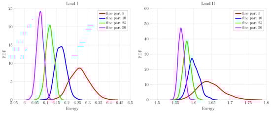
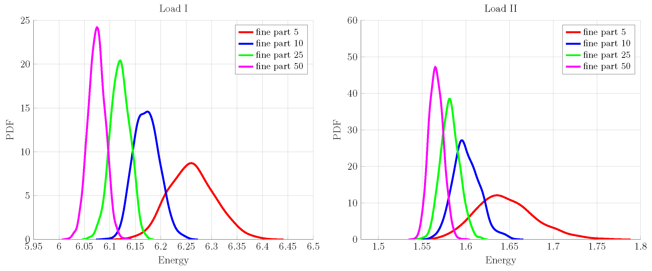
Figure 7.
Fine-scale energy PDFs for load cases (I,II) for different numbers of particles.
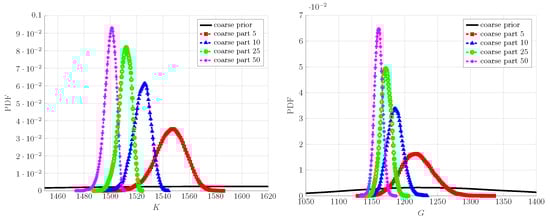
Figure 8.
Coarse-scale prior and posterior PDF for K and G using fine scale with different numbers of particles.
The PDFs of the updated coarse-scale parameters are shown in Figure 8. They exhibit a reduced degree of uncertainty as compared to the chosen prior. Moreover, the aleatoric uncertainty—observed in the response of fine-scale specimen with respect to the number of inclusions—is also reflected by the updated coarse scale i.e., the PDFs of K and G have a progressively increasing variance while going from 50 to 5 particles for fine-scale specimen. Finally, to demonstrate the validity of the updated coarse scale, the corresponding PDFs of energy posterior predictions are shown along with the fine-scale measurement ones in Figure 9. The up-scaled coarse-scale predictions match really well with the fine-scale measurement; the difference between the PDFs is unnoticeable for each inclusion case and the considered loading cases.
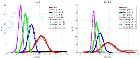
Figure 9.
Coarse-scale posterior predicted energy comparison with fine-scale measurements with different numbers of particles for load cases (I,II).
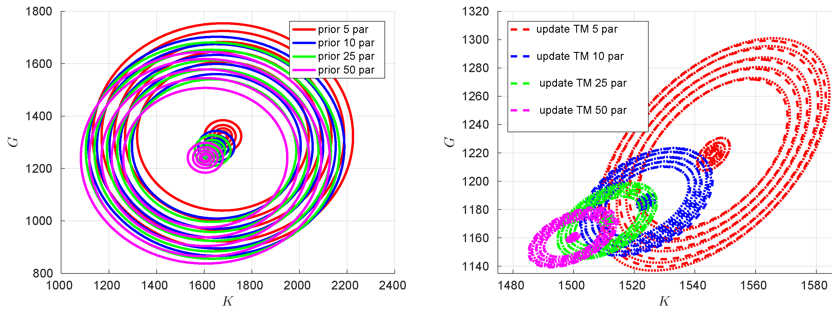
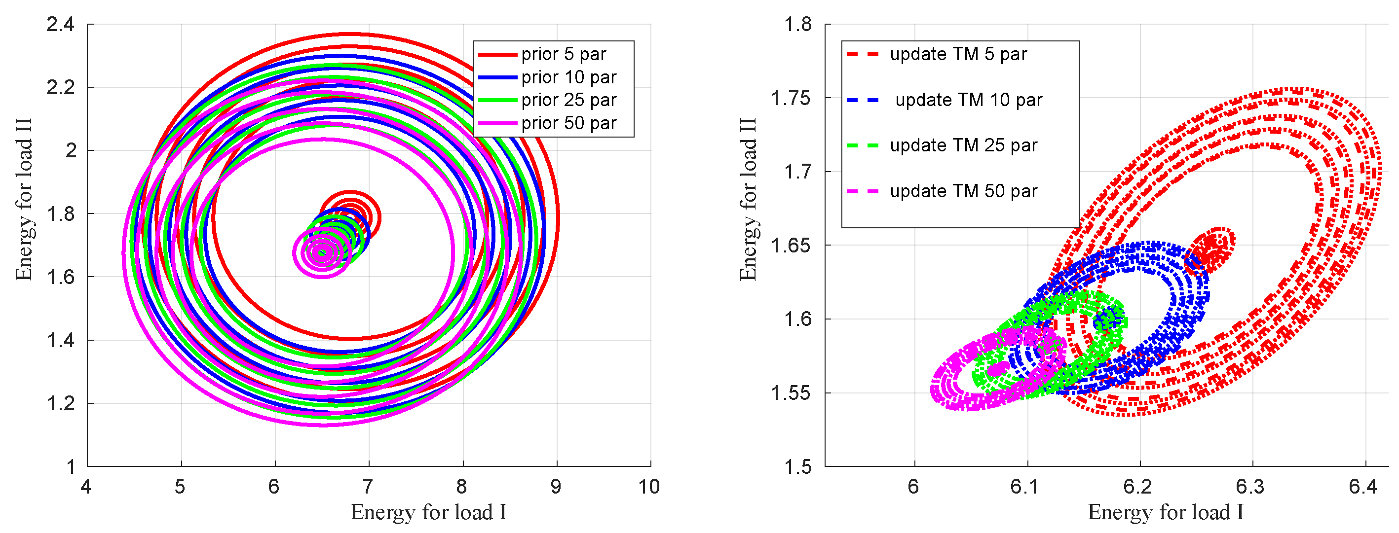
An interesting behavior, related to the up-scaling experiment, can be observed by examining the correlation between the prior and posterior material properties and the corresponding energy predictions in Figure 10 and Figure 11, respectively. Since K and G and the associated loading conditions, under consideration, are independent of each other (in particular for loading cases: hydrostatic compression and pure shear are mutually exclusive in terms of triggering volumetric and deviatoric deformations), the correlation for both (material properties and energies) prior are depicted as concentric circles in the left plots of Figure 10 and Figure 11 for different fine-scale particle configurations. The posterior or up-scaled coarse-scale properties and the corresponding energies correlations are shown on the right plots of Figure 10 and Figure 11, respectively. An obvious observation is that as one increases the number of particles, the variability decreases, which is also confirmed by the spread of distributions of up-scaled coarse-scale K and G, e.g., in Figure 8. Additionally, the correlation in the posterior coarse-scale properties and corresponding energy predictions are depicted as ellipses, from which one can conclude that the updated material parameters are correlated. The possible reason for correlated updated parameters is due to the geometric uncertainty (spatial position of particles) that is present in the considered RVs and is common for both types of loads.

Figure 10.
Correlation between prior and posterior (up-scaled) coarse-scale K and G considering all fine-scale particle cases.
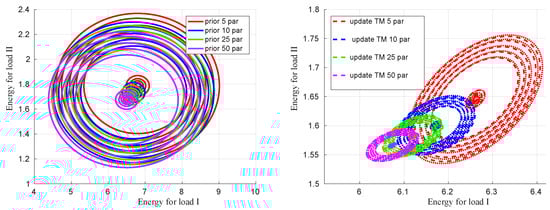
Figure 11.
Correlation between energies from load cases I and II using coarse-scale prior and up-scaled K and G considering all fine-scale particle cases.
6. Conclusions
In this paper, a Bayesian up-scaling framework is devised and is applied in a computational homogenization setting to estimate coarse-scale, homogenized material parameters that are representative of a more elaborate fine-scale material model. Moreover, the coarse and fine scales are assumed to be completely incomparable in terms of material description and their corresponding FEM simulation models; therefore, energy is used as the communication measure between the two scales, since it is representative of the physical behavior (e.g., elastic and inelastic phenomenon) common to both the scales. The algorithm is computationally efficient owing to the use of the functional approximation of involved quantities, and it is also non-intrusive: the PCE approximations are readily built from the ensemble of solutions obtained via the repeated execution of deterministic FEM solvers for the given random material samples. With regard to constructing PCE approximation for fine-scale energy, the construction of a transport map from energy samples has proved to be computationally efficient, as it allows to build PCE approximation directly from the energy samples and their transformed standard normal counterparts instead of using random samples to build fine-scale material realizations, which can be very expensive, owing to their high dimensionality, or impossible to build in the first place. The representative examples also show promising results as one is able to calibrate a continuum-based coarse-scale model using energy measurements from truss-based discrete fine-scale models. The reliability of the updated coarse-scale parameters is judged by comparing their energy predictions with the fine-scale ones. In both the cases, one realization and an ensemble of realizations, satisfactory results have been obtained under reasonable accuracy. The developed framework and the example study presented in this paper can be used as a platform to improve upon the existing algorithm and investigate more complex examples, e.g., incorporating inelastic or dissipative material behavior for up-scaling.
Author Contributions
B.V.R. proposed the idea; M.S.S. conducted the numerical implementation and simulations. Both M.S.S. and B.V.R. contributed to the writing part. H.G.M. writing, supervision, funding. All authors have read and agreed to the published version of the manuscript.
Funding
The support is provided by the German Science Foundation (Deutsche Forschungs-gemeinschaft, DFG) as part of priority programs SPP 1886 and SPP 1748.
Data Availability Statement
Data available upon request from the authors.
Conflicts of Interest
The authors declare no conflicts of interest.
Abbreviations
The following main abbreviations and mathematical symbols are used in this manuscript:
| FEM | finite element method |
| PCE | polynomial chaos expansion |
| gPCE | generalized polynomial chaos expansion |
| probability density function | |
| RV | random variable |
| QoI | quantity of interest |
| RVE | representative volume element |
| PINN | physics-informed neural networks |
| EnKF | ensemble Kalman Filter |
| state-space variables of coarse-scale model | |
| energy functional of coarse-scale model | |
| dissipation potential of coarse-scale model | |
| measurement noise associated with the fine-scale | |
| measurement and modelling error associated with coarse-scale model | |
| measurement operator of coarse scale | |
| material parameters of coarse-scale model | |
| external excitation on coarse level | |
| probability space of set of all events associated with RV | |
| probability measure associated with RV | |
| sigma-algebra | |
| sub-sigma-algebra | |
| RV used in computational scheme, taken as log of coase-scale material parameter . | |
| measurable map of RVs | |
| expectation operator | |
| Bregman’s loss function (BLF) or divergence between RVs | |
| hyperplane tangent to differentiable function at a given point | |
| set of n-th degree polynomials | |
| covariance matrix between RVs | |
| Kalman gain of PCE-based filter | |
| finite set of multi-indices with cardinality (size) Z | |
| Kullback–Leibler (KL) divergence between probability densities | |
| set of linearly independent functions for PCE | |
| coarse and fine-scale computational models | |
| cost function associated with transport map | |
| pushforward operator associated with transport map | |
| space of lower-triangular functions for transport map approximation | |
| probability measure of RV | |
| vector valued standard normal RVs | |
| covariance matrix in terms of PCE coefficients of | |
| deformation tensor | |
| Young modulli for particle and matrix truss elements |
References
- Feyel, F.; Chaboche, J.L. FE2 multiscale approach for modelling the elastoviscoplastic behaviour of long fibre SiC/Ti composite materials. Comput. Methods Appl. Mech. Eng. 2000, 183, 309–330. [Google Scholar] [CrossRef]
- Feyel, F. A multilevel finite element method (FE2) to describe the response of highly non-linear structures using generalized continua. Comput. Methods Appl. Mech. Eng. 2003, 192, 3233–3244. [Google Scholar] [CrossRef]
- Yvonnet, J.; Bonnet, G. A consistent nonlocal scheme based on filters for the homogenization of heterogeneous linear materials with non-separated scales. Int. J. Solids Struct. 2014, 51, 196–209. [Google Scholar] [CrossRef]
- Yvonnet, J.; Bonnet, G. Nonlocal/coarse-graining homogenization of linear elastic media with non-separated scales using least-square polynomial filters. Int. J. Multiscale Comput. Eng. 2014, 12, 375–395. [Google Scholar] [CrossRef]
- Ma, J.; Zhang, S.; Wriggers, P.; Gao, W.; De Lorenzis, L. Stochastic homogenized effective properties of three-dimensional composite material with full randomness and correlation in the microstructure. Comput. Struct. 2014, 144, 62–74. [Google Scholar] [CrossRef]
- Ma, J.; Sahraee, S.; Wriggers, P.; De Lorenzis, L. Stochastic multiscale homogenization analysis of heterogeneous materials under finite deformations with full uncertainty in the microstructure. Comput. Mech. 2015, 55, 819–835. [Google Scholar] [CrossRef]
- Ma, J.; Wriggers, P.; Li, L. Homogenized thermal properties of 3D composites with full uncertainty in the microstructure. Struct. Eng. Mech. 2016, 57, 369–387. [Google Scholar] [CrossRef]
- Ma, J.; Temizer, I.; Wriggers, P. Random homogenization analysis in linear elasticity based on analytical bounds and estimates. Int. J. Solids Struct. 2011, 48, 280–291. [Google Scholar] [CrossRef]
- Savvas, D.; Stefanou, G.; Papadrakakis, M. Determination of RVE size for random composites with local volume fraction variation. Comput. Methods Appl. Mech. Eng. 2016, 305, 340–358. [Google Scholar] [CrossRef]
- Savvas, D.; Stefanou, G. Determination of random material properties of graphene sheets with different types of defects. Compos. Part B Eng. 2018, 143, 47–54. [Google Scholar] [CrossRef]
- Stefanou, G.; Savvas, D.; Papadrakakis, M. Stochastic finite element analysis of composite structures based on material microstructure. Compos. Struct. 2015, 132, 384–392. [Google Scholar] [CrossRef]
- Stefanou, G. Simulation of heterogeneous two-phase media using random fields and level sets. Front. Struct. Civ. Eng. 2015, 9, 114–120. [Google Scholar] [CrossRef]
- Stefanou, G.; Savvas, D.; Papadrakakis, M. Stochastic finite element analysis of composite structures based on mesoscale random fields of material properties. Comput. Methods Appl. Mech. Eng. 2017, 326, 319–337. [Google Scholar] [CrossRef]
- Clément, A.; Soize, C.; Yvonnet, J. Computational nonlinear stochastic homogenization using a nonconcurrent multiscale approach for hyperelastic heterogeneous microstructures analysis. Int. J. Numer. Methods Eng. 2012, 91, 799–824. [Google Scholar] [CrossRef]
- Clément, A.; Soize, C.; Yvonnet, J. Uncertainty quantification in computational stochastic multiscale analysis of nonlinear elastic materials. Comput. Methods Appl. Mech. Eng. 2013, 254, 61–82. [Google Scholar] [CrossRef]
- Clément, A.; Soize, C.; Yvonnet, J. High-dimension polynomial chaos expansions of effective constitutive equations for hyperelastic heterogeneous random microstructures. In Proceedings of the Congress on Computational Methods in Applied Sciences and Engineering (ECCOMAS 2012), Vienna, Austria, 10–14 September 2012; Vienna University of Technology: Vienna, Austria, 2012; pp. 1–2. [Google Scholar]
- Staber, B.; Guilleminot, J. Functional approximation and projection of stored energy functions in computational homogenization of hyperelastic materials: A probabilistic perspective. Comput. Methods Appl. Mech. Eng. 2017, 313, 1–27. [Google Scholar] [CrossRef]
- Lu, X.; Giovanis, D.G.; Yvonnet, J.; Papadopoulos, V.; Detrez, F.; Bai, J. A data-driven computational homogenization method based on neural networks for the nonlinear anisotropic electrical response of graphene/polymer nanocomposites. Comput. Mech. 2019, 64, 307–321. [Google Scholar] [CrossRef]
- Ba Anh, L.; Yvonnet, J.; He, Q.C. Computational homogenization of nonlinear elastic materials using Neural Networks: Neural Networks-based computational homogenization. Int. J. Numer. Methods Eng. 2015, 104, 1061–1084. [Google Scholar] [CrossRef]
- Sagiyama, K.; Garikipati, K. Machine learning materials physics: Deep neural networks trained on elastic free energy data from martensitic microstructures predict homogenized stress fields with high accuracy. arXiv 2019, arXiv:1901.00524. Available online: http://arxiv.org/abs/1901.00524 (accessed on 15 November 2024).
- Unger, J.; Könke, C. An inverse parameter identification procedure assessing the quality of the estimates using Bayesian neural networks. Appl. Soft Comput. 2011, 11, 3357–3367. [Google Scholar] [CrossRef]
- Unger, J.; Könke, C. Coupling of scales in a multiscale simulation using neural networks. Comput. Struct. 2008, 86, 1994–2003. [Google Scholar] [CrossRef]
- Lizarazu, J.; Harirchian, E.; Shaik, U.A.; Shareef, M.; Antoni-Zdziobek, A.; Lahmer, T. Application of machine learning-based algorithms to predict the stress-strain curves of additively manufactured mild steel out of its microstructural characteristics. Results Eng. 2023, 20, 101587. [Google Scholar] [CrossRef]
- Logarzo, H.J.; Capuano, G.; Rimoli, J.J. Smart constitutive laws: Inelastic homogenization through machine learning. Comput. Methods Appl. Mech. Eng. 2021, 373, 113482. [Google Scholar] [CrossRef]
- Wang, K.; Sun, W. A multiscale multi-permeability poroplasticity model linked by recursive homogenizations and deep learning. Comput. Methods Appl. Mech. Eng. 2018, 334, 337–380. [Google Scholar] [CrossRef]
- Rixner, M.; Koutsourelakis, P.S. Self-supervised optimization of random material microstructures in the small-data regime. Npj Comput. Mater. 2022, 8, 46. [Google Scholar] [CrossRef]
- Frankel, A.; Jones, R.; Alleman, C.; Templeton, J. Predicting the mechanical response of oligocrystals with deep learning. Comput. Mater. Sci. 2019, 169, 109099. [Google Scholar] [CrossRef]
- Wang, K.; Sun, W. Meta-modeling game for deriving theory-consistent, microstructure-based traction–separation laws via deep reinforcement learning. Comput. Methods Appl. Mech. Eng. 2019, 346, 216–241. [Google Scholar] [CrossRef]
- Raissi, M.; Perdikaris, P.; Karniadakis, G. Physics-informed neural networks: A deep learning framework for solving forward and inverse problems involving nonlinear partial differential equations. J. Comput. Phys. 2019, 378, 686–707. [Google Scholar] [CrossRef]
- Haghighat, E.; Raissi, M.; Moure, A.; Gomez, H.; Juanes, R. A physics-informed deep learning framework for inversion and surrogate modeling in solid mechanics. Comput. Methods Appl. Mech. Eng. 2021, 379, 113741. [Google Scholar] [CrossRef]
- Chen, C.T.; Gu, G.X. Physics-Informed Deep-Learning For Elasticity: Forward, Inverse, and Mixed Problems. Adv. Sci. 2023, 10, 2300439. [Google Scholar] [CrossRef]
- Xu, K.; Tartakovsky, A.M.; Burghardt, J.; Darve, E. Inverse modeling of viscoelasticity materials using physics constrained learning. arXiv 2020, arXiv:2005.04384. [Google Scholar]
- Tartakovsky, A.M.; Marrero, C.O.; Perdikaris, P.; Tartakovsky, G.D.; Barajas-Solano, D. Learning parameters and constitutive relationships with physics informed deep neural networks. arXiv 2018, arXiv:1808.03398. [Google Scholar]
- Haghighat, E.; Abouali, S.; Vaziri, R. Constitutive model characterization and discovery using physics-informed deep learning. Eng. Appl. Artif. Intell. 2023, 120, 105828. [Google Scholar] [CrossRef]
- Rojas, C.J.; Boldrini, J.L.; Bittencourt, M.L. Parameter identification for a damage phase field model using a physics-informed neural network. Theor. Appl. Mech. Lett. 2023, 13, 100450. [Google Scholar] [CrossRef]
- Maia, M.; Rocha, I.; Kerfriden, P.; van der Meer, F. Physically recurrent neural networks for path-dependent heterogeneous materials: Embedding constitutive models in a data-driven surrogate. Comput. Methods Appl. Mech. Eng. 2023, 407, 115934. [Google Scholar] [CrossRef]
- Rocha, I.; Kerfriden, P.; van der Meer, F. Machine learning of evolving physics-based material models for multiscale solid mechanics. Mech. Mater. 2023, 184, 104707. [Google Scholar] [CrossRef]
- Borkowski, L.; Skinner, T.; Chattopadhyay, A. Woven ceramic matrix composite surrogate model based on physics-informed recurrent neural network. Compos. Struct. 2023, 305, 116455. [Google Scholar] [CrossRef]
- Flaschel, M.; Kumar, S.; De Lorenzis, L. Unsupervised discovery of interpretable hyperelastic constitutive laws. Comput. Methods Appl. Mech. Eng. 2021, 381, 113852. [Google Scholar] [CrossRef]
- Wang, Z.; Estrada, J.; Arruda, E.; Garikipati, K. Inference of deformation mechanisms and constitutive response of soft material surrogates of biological tissue by full-field characterization and data-driven variational system identification. J. Mech. Phys. Solids 2021, 153, 104474. [Google Scholar] [CrossRef]
- Flaschel, M.; Kumar, S.; De Lorenzis, L. Automated discovery of generalized standard material models with EUCLID. Comput. Methods Appl. Mech. Eng. 2023, 405, 115867. [Google Scholar] [CrossRef]
- Flaschel, M.; Kumar, S.; De Lorenzis, L. Discovering plasticity models without stress data. Npj Comput. Mater. 2022, 8, 91. [Google Scholar] [CrossRef]
- Joshi, A.; Thakolkaran, P.; Zheng, Y.; Escande, M.; Flaschel, M.; De Lorenzis, L.; Kumar, S. Bayesian-EUCLID: Discovering hyperelastic material laws with uncertainties. Comput. Methods Appl. Mech. Eng. 2022, 398, 115225. [Google Scholar] [CrossRef]
- Koutsourelakis, P.S. Stochastic upscaling in solid mechanics: An excercise in machine learning. J. Comput. Phys. 2007, 226, 301–325. [Google Scholar] [CrossRef]
- Schöberl, M.; Zabaras, N.; Koutsourelakis, P.S. Predictive Collective Variable Discovery with Deep Bayesian Models. arXiv 2018, arXiv:1809.06913. [Google Scholar] [CrossRef]
- Felsberger, L.; Koutsourelakis, P.S. Physics-constrained, data-driven discovery of coarse-grained dynamics. arXiv 2018, arXiv:1802.03824. [Google Scholar]
- Sarfaraz, S.M.; Rosić, B.V.; Matthies, H.G.; Ibrahimbegović, A. Bayesian stochastic multi-scale analysis via energy considerations. arXiv 2019, arXiv:1912.03108. [Google Scholar] [CrossRef]
- Sarfaraz, S.M.; Rosić, B.V.; Matthies, H.G.; Ibrahimbegović, A. Stochastic upscaling via linear Bayesian updating. In Multiscale Modeling of Heterogeneous Structures; Springer: Berlin/Heidelberg, Germany, 2018; pp. 163–181. [Google Scholar]
- Rosić, B.V. Stochastic state estimation via incremental iterative sparse polynomial chaos based Bayesian-Gauss-Newton-Markov-Kalman filter. arXiv 2019, arXiv:1909.07209. [Google Scholar]
- Marzouk, Y.; Moselhy, T.; Parno, M.; Spantini, A. Sampling via Measure Transport: An Introduction. In Handbook of Uncertainty Quantification; Springer International Publishing: Cham, Swizterland, 2016; pp. 1–41. [Google Scholar] [CrossRef]
- Parno, M.D. Transport Maps for Accelerated Bayesian Computation. Ph.D. Thesis, Massachusetts Institute of Technology, Cambridge, MA, USA, 2015. [Google Scholar]
- Parno, M.D.; Marzouk, Y.M. Transport Map Accelerated Markov Chain Monte Carlo. SIAM/ASA J. Uncertain. Quantif. 2018, 6, 645–682. [Google Scholar] [CrossRef]
- Mielke, A.; Roubíček, T. Rate Independent Systems: Theory and Application; Springer: New York, NY, USA, 2015. [Google Scholar]
- Barbu, A.; Zhu, S.C. Monte Carlo Methods; Springer Nature: Singapore, 2020. [Google Scholar]
- Banerjee, A.; Guo, X.; Wang, H. On the Optimality of Conditional Expectation as a Bregman Predictor. Inf. Theory IEEE Trans. 2005, 51, 2664–2669. [Google Scholar] [CrossRef]
- Matthies, H.G.; Zander, E.; Rosić, B.V.; Litvinenko, A.; Pajonk, O. Inverse Problems in a Bayesian Setting; Springer International Publishing: Cham, Swizterland, 2016; pp. 245–286. [Google Scholar] [CrossRef]
- Xiu, D. Numerical Methods for Stochastic Computations: A Spectral Method Approach; Princeton University Press: Princeton, NJ, USA, 2010. [Google Scholar]
- Rojo-Alvarez, J.L.; Martínez-Ramón, M.; Muňoz-Marí, J.; Camps-Valls, G. Digital Signal Processing with Kernel Methods; IEEE Press, Wiley: Hoboken, NJ, USA, 2018. [Google Scholar]
- Buhmann, M.D. Radial Basis Functions: Theory and Implementations; Cambridge Monographs on Applied and Computational Mathematics; Cambridge University Press: London, UK, 2003. [Google Scholar]
- Zimmermann, H.J. Fuzzy set theory. WIREs Comput. Stat. 2010, 2, 317–332. [Google Scholar] [CrossRef]
- Matthies, H.G. Stochastic finite elements: Computational approaches to stochastic partial differential equations. Z. für Angew. Math. und Mech. (ZAMM) 2008, 88, 849–873. [Google Scholar] [CrossRef]
- Rosić, B.V.; Matthies, H.G. Variational Theory and Computations in Stochastic Plasticity. Arch. Comput. Methods Eng. 2015, 22, 457–509. [Google Scholar] [CrossRef]
- Blatman, G.; Sudret, B. Adaptive sparse polynomial chaos expansion based on least angle regression. J. Comput. Phys. 2011, 230, 2345–2367. [Google Scholar] [CrossRef]
- Oladyshkin, S.; Nowak, W. Data-driven uncertainty quantification using the arbitrary polynomial chaos expansion. Reliab. Eng. Syst. Saf. 2012, 106, 179–190. [Google Scholar] [CrossRef]
- Villani, C. Optimal Transport: Old and New; Grundlehren der mathematischen Wissenschaften; Springer: Berlin/Heidelberg, Germany, 2008. [Google Scholar]
- Galichon, A. Optimal Transport Methods in Economics; Princeton University Press: Princeton, NJ, USA, 2018. [Google Scholar]
- Dominitz, A.; Angenent, S.; Tannenbaum, A. On the Computation of Optimal Transport Maps Using Gradient Flows and Multiresolution Analysis. In Proceedings of the Recent Advances in Learning and Control; Blondel, V.D., Boyd, S.P., Kimura, H., Eds.; Springer: London, UK, 2008; pp. 65–78. [Google Scholar]
- Brenier, Y. Optimal transportation of particles, fluids and currents. In Variational Methods for Evolving Objects; Mathematical Society of Japan (MSJ): Tokyo, Japan, 2015; pp. 59–85. [Google Scholar] [CrossRef]
- Solomon, J.; De Goes, F.; Peyré, G.; Cuturi, M.; Butscher, A.; Nguyen, A.; Du, T.; Guibas, L. Convolutional wasserstein distances: Efficient optimal transportation on geometric domains. ACM Trans. Graph. (TOG) 2015, 34, 66. [Google Scholar] [CrossRef]
- Bonneel, N.; van de Panne, M.; Paris, S.; Heidrich, W. Displacement Interpolation Using Lagrangian Mass Transport. ACM Trans. Graph. 2011, 30, 158:1–158:12. [Google Scholar] [CrossRef]
- Genevay, A.; Cuturi, M.; Peyré, G.; Bach, F. Stochastic Optimization for Large-scale Optimal Transport. In Advances in Neural Information Processing Systems 29; Lee, D.D., Sugiyama, M., Luxburg, U.V., Guyon, I., Garnett, R., Eds.; Curran Associates, Inc.: Red Hook, NY, USA, 2016; pp. 3440–3448. [Google Scholar]
- Cuturi, M. Sinkhorn distances: Lightspeed computation of optimal transport. In Proceedings of the Advances in Neural Information Processing Systems, Lake Tahoe, NV, USA, 5–10 December 2013; pp. 2292–2300. [Google Scholar]
- Henderson, T.; Solomon, J. Audio Transport: A Generalized Portamento via Optimal Transport. 2019. Available online: http://arxiv.org/abs/1906.06763 (accessed on 15 November 2024).
- Dessein, A.; Papadakis, N.; Deledalle, C.A. Parameter estimation in finite mixture models by regularized optimal transport: A unified framework for hard and soft clustering. arXiv 2017, arXiv:1711.04366. [Google Scholar]
- Genevay, A.; Peyré, G.; Cuturi, M. GAN and VAE from an optimal transport point of view. arXiv 2017, arXiv:1706.01807. [Google Scholar]
- Eigel, M.; Gruhlke, R.; Marschall, M. Low-rank tensor reconstruction of concentrated densities with application to Bayesian inversion. Stat. Comput. 2022, 32, 27. [Google Scholar] [CrossRef]
- Spantini, A.; Bigoni, D.; Marzouk, Y. Inference via low-dimensional couplings. J. Mach. Learn. Res. 2018, 19, 2639–2709. [Google Scholar]
- Huan, X. Numerical Approaches for Sequential Bayesian Optimal Experimental Design. Ph.D. Thesis, Massachusetts Institute of Technology, Cambridge, MA, USA, 2015. [Google Scholar]
- Deuflhard, P. Newton Methods for Nonlinear Problems: Affine Invariance and Adaptive Algorithms; Springer Series in Computational Mathematics; Springer: Berlin/Heidelberg, Germany, 2011. [Google Scholar]
- Benkemoun, N. Contribution aux Approches Multi-échelles Séquencées pour la Modélisation Numérique des Matériaux à Matrice Cimentaire. Ph.D. Thesis, Ècole Normale Supérieure Paris-Saclay, Cachan, France, 2010. [Google Scholar]
- Benkemoun, N.; Ibrahimbegović, A.; Colliat, J.B. Anisotropic constitutive model of plasticity capable of accounting for details of meso-structure of two-phase composite material. Comput. Struct. 2012, 90, 153–162. [Google Scholar] [CrossRef]
- Benkemoun, N.; Hautefeuille, M.; Colliat, J.B.; Ibrahimbegović, A. Failure of heterogeneous materials: 3D meso-scale FE models with embedded discontinuities. Int. J. Numer. Methods Eng. 2010, 82, 1671–1688. [Google Scholar] [CrossRef]
- Taylor, R. FEAP—Finite Element Analysis Program; University of California: Berkeley, CA, USA, 2014. [Google Scholar]
- The MathWorks Inc. MATLAB Version: 9.13.0 (R2022b). (The MathWorks Inc., 2022). Available online: https://www.mathworks.com (accessed on 5 October 2024).
- Torquato, S. Random Heterogeneous Materials: Microstructure and Macroscopic Properties; Interdisciplinary Applied Mathematics; Springer: New York, NY, USA, 2005. [Google Scholar]
- Bigoni, D.; Spantini, A.; Morrisno, R.; Baptista, R.; Marzouk, Y. TransportMaps v2.0. 2018. Available online: http://transportmaps.mit.edu/ (accessed on 20 October 2024).
- Ostoja-Starzewski, M. Microstructural Randomness and Scaling in Mechanics of Materials; Modern Mechanics and Mathematics; CRC Press: Boca Raton, FL, USA, 2007. [Google Scholar]
Disclaimer/Publisher’s Note: The statements, opinions and data contained in all publications are solely those of the individual author(s) and contributor(s) and not of MDPI and/or the editor(s). MDPI and/or the editor(s) disclaim responsibility for any injury to people or property resulting from any ideas, methods, instructions or products referred to in the content. |
© 2025 by the authors. Licensee MDPI, Basel, Switzerland. This article is an open access article distributed under the terms and conditions of the Creative Commons Attribution (CC BY) license (https://creativecommons.org/licenses/by/4.0/).