Tree-Based Methods of Volatility Prediction for the S&P 500 Index

Abstract

Predicting asset return volatility is one of the central problems in quantitative finance. These predictions are used for portfolio construction, calculation of value at risk (VaR), and pricing of derivatives such as options. Classical methods of volatility prediction utilize historical returns data and include the exponentially weighted moving average (EWMA) and generalized autoregressive conditional heteroskedasticity (GARCH). These approaches have shown significantly higher rates of predictive accuracy than corresponding methods of return forecasting, but they still have vast room for improvement. In this paper, we propose and test several methods of volatility forecasting on the S&P 500 Index using tree ensembles from machine learning, namely random forest and gradient boosting. We show that these methods generally outperform the classical approaches across a variety of metrics on out-of-sample data. Finally, we use the unique properties of tree-based ensembles to assess what data can be particularly useful in predicting asset return volatility.

1. Introduction

1.1. Overview

Finance acquired its most elemental measurements from statistics, including metrics such as mean, standard deviation, and correlation. Mean became the measure of average returns over some period of time and, if applied to the future, of expected return. Standard deviation or its squared analog, variance, came to measure the dispersion of returns around the mean [1]. This metric took on the name volatility, and it holds a crucial place in much of modern finance. Equation (1) defines the sample standard deviation, or volatility, where r_t is a given realized return from a time series, while $\overline{\mathrm{r}}$ is the sample mean of the series and n is the length of the series.

$$s=\sqrt{{\displaystyle \frac{{\sum }_{t=1}^n{\left(r_t-\overline{r}\right)}^2}{n-1}}}$$

(1)

While a higher expected return is almost always desired in an asset or a portfolio, higher volatility is usually something to avoid—indeed, the standard mean–variance optimization framework explicitly penalizes variance in a portfolio by equating it with risk [2]. Volatility is a central component of most risk management systems and is related to tail risk measures like value at risk and expected shortfall. The pricing of options and many other derivatives also necessitates volatility, as originally described by Black and Scholes [3]. In these and other applications, what matters is typically not historical volatility but future realization. Fortunately, financial academics and practitioners have long known that future volatility is more persistent than future returns [4], a finding sometimes known as volatility clustering. To take advantage of this relative persistence, there is a number of “classical” methods, such as simple moving averages, exponentially weighted moving averages, and the ARCH/GARCH family of models. For assets with liquid options, one could also calculate the implied volatility of the options from market prices, though this does not answer how market participants set the options prices in the first place.

Our contribution is to improve on the existing methods by introducing the use of tree-based machine learning ensembles such as random forest and gradient boosting. These non-parametric methods were developed outside of finance and economics but have achieved impressive results when applied to forecasting in a variety of fields. More specifically, we use recent daily returns to predict 21-day-ahead volatility, which corresponds to one month’s worth of trading days. While tree-based methods have been applied to return prediction [5,6], we believe we are the first to apply these approaches for volatility prediction. We show that tree ensembles, particularly gradient boosting, can produce superior volatility forecasts for the S&P 500, one of the most popular stock indices in the United States. We also show that even better results can be obtained by combining historical returns data with a market-based volatility estimate in the form of the CBOE VIX Index. All of these results are calculated on out-of-sample test data temporally separated from the training data used to build the models. We do not necessarily claim that these tree-based methods generalize to all financial assets, and future research would be needed to confirm or refute such a claim. Finally—and most uniquely—we look “under the hood” of our random forest and gradient boosting models to understand the time lags that are especially significant for volatility forecasts. We find strong evidence for the exponentially decaying relevance of older data, similar to EWMA. Therefore, improved accuracy of tree-based methods likely results from their ability to process data in a non-linear way.

1.2. Literature Review

Simple methods of volatility forecasting include trailing moving averages of recent volatility, e.g., using realized volatility over the past x days as a prediction of volatility over the next y days. This assumes that the near future will resemble the near past, an often-reasonable assumption given the tendency of volatility to cluster across time. A more sophisticated and often more accurate approach is the exponentially weighted moving average (EWMA), which gives more recent observations a greater weight compared to older observations [7]. Equation (2) shows the EWMA-predicted variance as a function of realized returns (r_t), the mean of the returns (μ_t, sometimes assumed to be 0), and a decay factor (δ) that ranges between 0 and 1.

$${\mathsf{\sigma }}_t^2={\displaystyle \frac{\left(1-\mathsf{\delta }\right)}{\left(1-{\mathsf{\delta }}^n\right)}}{\sum }_{i=0}^{n-1}{\mathsf{\delta }}^i{\left(r_{t-i}-\mathsf{\mu }\right)}^2$$

(2)

$$A={\displaystyle \frac{S_1}{S_1^2-S_2}}$$

$$B=S_{1}A$$

$$S_1={\displaystyle \frac{1-{\mathsf{\delta }}^n}{1-\mathsf{\delta }}}$$

$$S_2={\displaystyle \frac{1-{\mathsf{\delta }}^{2n}}{1-{\mathsf{\delta }}^2}}$$

The field of econometrics advanced the prediction of volatility with the introduction of the autoregressive conditional heteroskedasticity (ARCH) model by Engle [8]. ARCH forecasts future variance based on long-run variance and recent disturbances. Bollerslev [9] extended the framework to include lags of previous predictions, creating the popular generalized autoregressive conditional heteroskedasticity (GARCH) model, whose one-lag version is seen in Equation (3). The model estimates three coefficients that should sum to one: α₀ for long-run variance, α₁ for lagged values of the residual, and β for lagged values of predicted variance. GARCH allows for additional lags of either the autoregressive term or the residual term or both, though the functional form is always additive. Later, researchers created a vast number of additional refinements to GARCH, such as the exponential (EGARCH), integrated (IGARCH), fractionally integrated (FIGARCH), threshold (TGARCH), and other versions (for a typical comparison, see [10]). Most modern commercial software packages for the forecasting of volatility use a variant of either GARCH or EWMA.

$${\mathsf{\sigma }}_t^2={\mathsf{\alpha }}_0\overline{{\mathsf{\sigma }}^2}+{\mathsf{\alpha }}_1{\mathsf{\sigma }}_{t-1}^2{u}_{t-1}^2+\mathsf{\beta }{\mathsf{\sigma }}_{t-1}^2$$

(3)

In recent years, academics have published numerous new approaches to volatility prediction. Corsi [11] introduced the heterogeneous autoregressive (HAR) model, which posits that a linear cascade of daily, weekly, and monthly values of realized volatility can predict future volatility. Other regression-based approaches use macro variables to augment returns data, as reviewed by Zeng et al. [12]. As part of the deep learning boom of the last decade, models like those of Bucci [13] have utilized various neural network architectures for financial market forecasting. New approaches also sometimes incorporate data beyond historical returns, such as Internet search frequency [14]. While deep learning approaches have reported strong results in volatility prediction, they suffer from the “black box” problem of limited insight into how and why they work. Still, other research has used intraday returns as inputs, which is generally not feasible for the classical models [15].

Machine learning originated in the mid-twentieth century at the intersection of the fields of statistics and computer science. Its goal was the development of algorithms that could “learn” patterns in training data, often for purposes of prediction based on previously unseen data. Decades of research have produced many approaches, including penalized linear models, support vector machines, neural networks, and more [16]. An important strand of machine learning research started with the introduction of classification and regression trees (CART) by Breiman et al. [17]. A CART builds a binary tree where each split is a certain feature of the data at a certain cutoff point, as shown in Figure 1 below. The algorithm chooses the features and cutoff points by minimizing a loss function, such as mean squared error for regression and Gini impurity for classification. This means CART is a greedy algorithm, making the locally optimal choice at each stage. The added step of pruning the tree by deleting nodes with small sample sizes can reduce overfitting.

While individual trees offer a highly tractable method of machine learning, they typically perform poorly compared to other methods. To remedy this defect, Breiman introduced the idea of tree ensembles, or models composed of many trees. In bootstrap aggregation, or bagging, a preset number of trees are built on bootstrapped versions of the original dataset [19]. Though each tree may have a high error rate, the aggregate of all the predictions is typically much more accurate. Breiman [20] further improved on bagging by selecting features at each split point from a random subset of all features, known as a random forest. Despite being somewhat counterintuitive, this method combats overfitting of the training data by occasionally forcing the model to use features it may otherwise ignore. The model builder must set the number of features to sample from at each split point, a tunable hyperparameter often denoted as mtry. Other tunable hyperparameters in typical random forest models include maximum tree depth, minimal sample size for a node, the exact splitting rule to use, etc.

A random forest builds numerous trees in parallel, but the gradient boosting approach proposed by Friedman [21] builds trees in sequence. While the first tree is fit to the observed data, each subsequent tree is fit to the residuals of the prior tree. Often, the individual trees only consist of a root and two nodes, and the model’s predictive power comes entirely from the sequential construction of trees. Much like random forests, gradient boosting requires several tunable hyperparameters, such as tree depth, learning rate, and the total number of trees. When done correctly, this can prevent overfitting by pushing the model to learn more general patterns instead of simply memorizing the training data. As with most methods of machine learning, tuning is typically done with n-fold cross-validation, while the final model is evaluated on a test set of data it has not seen before.

2. Materials and Methods

2.1. Preliminary Decisions

To offer a fair comparison between classical methods and our approach, we limit ourselves to daily returns, as opposed to using intraday returns. More specifically, the daily returns are the percentage change in the S&P 500 price index according to closing values. Instead of calculating new features from our data, such as the trailing volatilities in the HAR model, we leave the daily returns as the predictors; this will become significant when we analyze feature importance. We employ the following conventions for trading days: 21 trading days in a month, 93 in a quarter, 126 in six months, and 252 in a full year. Finally, all standard deviation statistics are reported as annualized numbers, which necessitates scaling by the square root of time.

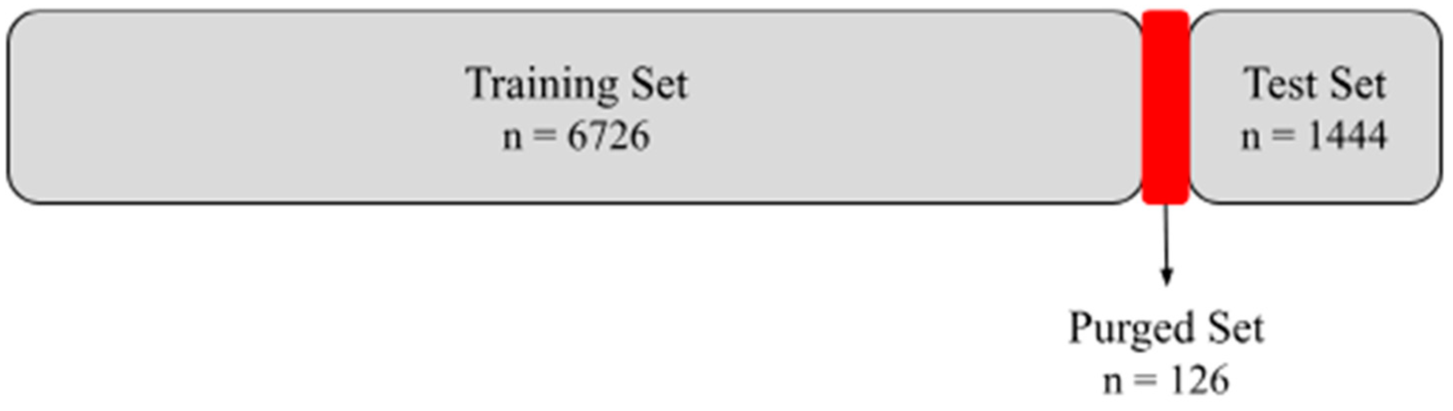
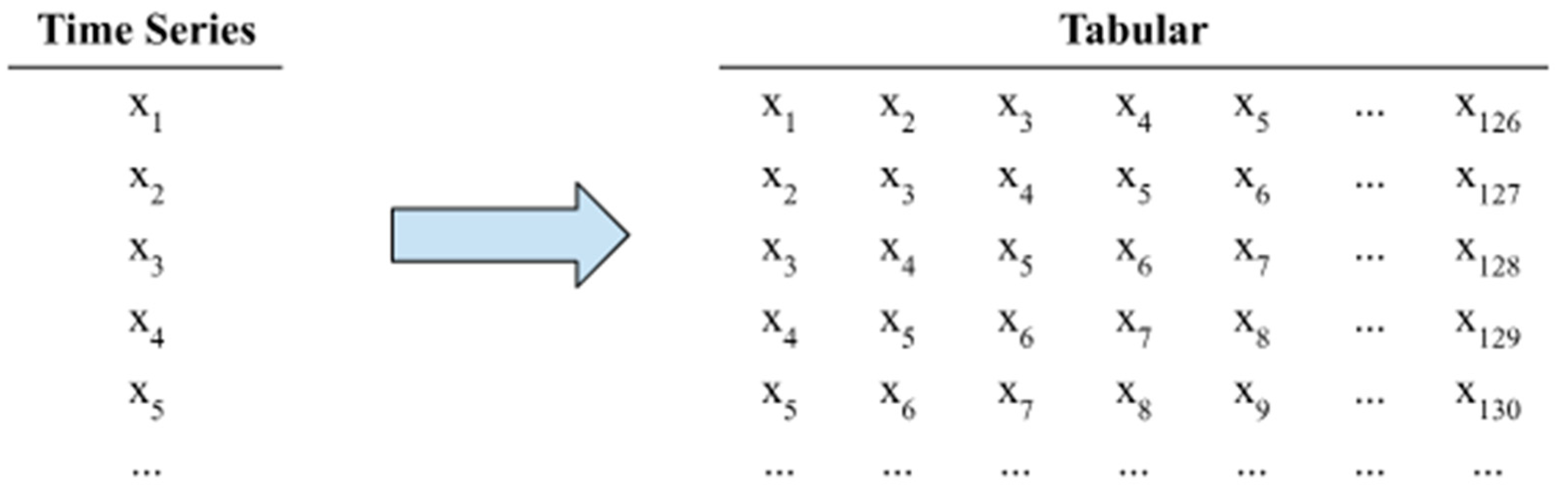
2.2. Data and Preprocessing

Our full dataset consists of 31 years of daily returns for the S&P 500 Index, a very popular capitalization-weighted index of stocks traded in the United States; our full time series begins in February 1993 and ends in March 2024. While the S&P 500 has historical data starting in the 1950s, we restrict the sample to a more recent period due to the possibility that older data are less relevant to modern markets. Beginning in the early 1990s allows us to capture the entirety of the current era of globalized markets, though any chosen starting point will be somewhat arbitrary. We partition our 7846 data points into three non-overlapping pieces—a training set, a purged set, and a test set—as depicted in Figure 2 below. While the training set and test set are standard in machine learning, the purged set is somewhat unusual and follows the recommendation of Lopez de Prado [22]. In time-series data like ours, serial correlation can lead to informational leakage when the test data directly follow the training data. By “purging”, or discarding, data between the two sets, we can reduce this risk and protect the validity of our conclusions. We purge 126 data points, or six months of daily data, for reasons we will soon explain.

Tree-based methods generally accept data in tabular form, with rows corresponding to individual samples and columns corresponding to features of the data. To accommodate the format, we take “slices” (also called windows) of our data in both the training and test sets, with each slice taking up one row and consisting of 126 consecutive daily returns. This means our features are the daily returns themselves—one for each trading day in a six-month period. There is nothing special about 126 days of trading data, but this period should be long enough to capture autocorrelation in volatility without being so long that older data are irrelevant. Consecutive slices share 124 of 126 data points, as using non-overlapping slices would lead to a sample size of only 62. While the 126 daily returns serve as our features, our target for prediction is the sample standard deviation of returns for the subsequent 21 days, as calculated in Equation (1). Figure 3 provides a visual depiction of the slicing process, which we use on both the training and test sets. We purged exactly 126 data points between our training and test sets because that is the length of one of our data slices. Finally, we note that there is very little collinearity among our features, with the highest correlation between any two columns in the training data being 0.04.

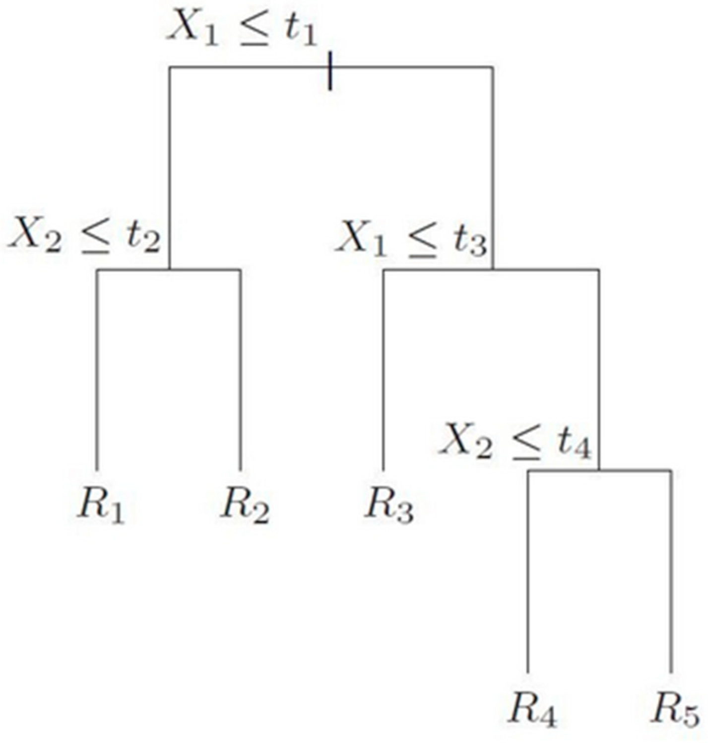
2.3. Prediction Methods

Using the R programming language and associated libraries, we examine seven total methods of volatility prediction—three classical, one using options, and three based on decision trees. The first method is an equally weighted moving average of past values. This simply involves calculating the realized volatility of the final 21 days of each data slice and using it as the prediction for the following 21 days, as seen in Equation (1); it implicitly assumes that each day in the past contributes an equal amount of information. The second method utilizes an exponentially weighted moving average, as seen in Equation (2). The EWMA uses all 126 available data points in each data slice, but it weights the more recent data points more heavily. We tune the important decay factor (δ) hyperparameter with 10-fold cross-validation on the training data, using mean squared error (MSE) as the value to minimize. The final classical prediction approach is a GARCH (1,1) model found in Equation (3). As GARCH generally requires more than 100 specified data points, we use the full training time series instead of relying on slices. Our options-based prediction method is based on the CBOE VIX Index, which tracks implied volatility of at-the-money one-month options on the S&P 500 Index. For each of the 21-day prediction periods, our volatility forecast is simply the closing value of the VIX on the day before the prediction period started.

The first decision tree method is random forest, for which we employ 500 trees without a limit on tree depth. The sole hyperparameter to tune through 10-fold cross-validation is the number of features to sample at each split point; we select this value by performing a grid search with options ranging from 10 to 120 in increments of 10. Intuitively, this corresponds to using either a small subset of historical data (10 days out of 126 possible days), a large subset, or some intermediate value. The lack of limit on tree depth makes this a computationally intensive model, so we use 20 parallel CPU cores to speed up the calculations. The second decision tree method is XGBoost (version 1.7.5.1), a variant of gradient boosting. We tune two hyperparameters using 10-fold cross-validation: the learning rate of the model and the total number of trees; the learning rate varies from 0.05 to 0.30 in increments of 0.05, while the number of trees ranges from 50 to 500 in steps of 50. We set the maximum tree depth to one, though we could also tune this as well. Our final method is also gradient boosting using XGBoost but with the addition of the VIX value as another predictor, in addition to the 126 historical daily returns. While there are many ways to combine forecasts, we favor this approach because it allows the gradient boosting model to determine the relative importance of VIX versus the historical data. Our tuning procedure for gradient boosting + VIX is the same as for regular gradient boosting.

2.4. Evaluation Metrics

Our goal throughout this paper is to predict the future volatility (standard deviation) of returns, a continuous and real-valued quantity. We use three metrics to evaluate the performance of all the tested models, the first of which is root mean squared error (RMSE), as seen in Equation (4). RMSE is a very common measure of success for regression tasks, but we supplement it with mean absolute error (MAE), as shown in Equation (5). MAE is similarly concerned with average errors, but its use of absolute values reduces the impact of outliers compared to RMSE. Finally, we use mean absolute percentage error (MAPE), a scaled metric defined in Equation (6). In Equations (4)–(6), y_i is the true value of volatility, while ŷ_i is the predicted value.

$$RMSE=\sqrt{{\displaystyle \frac{{\sum }_{i=1}^N{\left(y_i-\widehat{y_i}\right)}^2}{N}}}$$

(4)

$$MAE={\displaystyle \frac{{\sum }_{i=1}^N\left|y_i-\widehat{y_i}\right|}{N}}$$

(5)

$$MAPE={\displaystyle \frac{1}{n}}{\sum }_{i=1}^n{\displaystyle \frac{\left|y_i-\widehat{y_i}\right|}{y_i}}$$

(6)

3. Results

3.1. Forecast Comparisons

Table 1. Comparison of forecast methods. Bolded values indicate lowest scores (best).

Method	Hyperparameters	RMSE	MAE	MAPE
Simple Moving Average	Lookback = 21 days	12.3%	6.7%	38.3%
EWMA	δ = 0.88	11.5%	6.5%	36.4%
GARCH	(p, q) = (1, 1)	12.2%	7.2%	32.4%
VIX		10.6%	6.9%	48.0%
Random Forest	mtry = 30, trees = 500	9.9%	5.2%	31.5%
Gradient Boosting	eta = 0.1, trees = 450	9.6%	5.3%	31.1%
Gradient Boosting + VIX	eta = 0.1, trees = 250	9.5%	5.0%	29.0%

below shows the performance of each of the seven methods across the three metrics; all numbers are calculated on the out-of-sample test set, and lower values are always better. One result is that none of the classical methods clearly dominates the others. The simple moving average has the worst RMSE but has a lower MAE than GARCH. EWMA improves on the simple moving average across all metrics, but the improvement is generally small. GARCH has a high RMSE and MAE but lower MAPE than the moving averages; this is because it is more likely to underestimate volatility, and MAPE penalizes underestimation less than overestimation. Using the VIX, which requires no modeling or calculations, results in a lower RMSE than the classical methods, an average MAE, and the worst MAPE among all models. We believe this is because the VIX is more successful at predicting outlier values of volatility, especially very high values during periods of market stress. However, its average predictions are higher than those of other models due to the volatility risk premium in options [23], resulting in a poor MAPE. The random forest clearly beats the classical methods and VIX, while gradient boosting comes ahead of random forest on RMSE and MAPE. However, overall, the best model across all metrics is the final one—gradient boosting with the addition of VIX as another predictor.

3.2. Variable Importance

Tree-based methods of machine learning allow for a degree of insight into how the model makes its predictions. For random forests and gradient boosting, we can answer this question through variable importance analysis. Each time a tree is split, the variable importance algorithm tracks the splitting predictor, as well as how much the sum of squared errors (SSE) is reduced. By averaging across all created trees, variable importance produces a relative ranking of all the predictors. Figure 4 illustrates the variable importance measures for our three tree-based models and compares them to EWMA weights.

In the random forest and both versions of gradient boosting, recent returns are far more predictive of future volatility than returns at the start of the 126-day period. The decline in variable importance as returns recede further into the past is largely consistent with exponential decay, possibly explaining why EWMA is a popular choice for volatility prediction. However, both our random forest model and the gradient boosting model (without VIX) meaningfully outperform EWMA, suggesting that the tree ensembles add predictive power. We think this is due to the non-linear nature of tree ensembles; while EWMA and GARCH are confined to relatively simple, additive representations of volatility, deep and independent trees (as in random forest) or small sequential trees (as in gradient boosting) can capture more complex patterns in historical returns data. In addition, the binary nature of regression trees allows the models to learn differences between historical returns above the mean and those below the mean. Finally, in the gradient boosting model including VIX, we see that the VIX itself is the dominant explanatory variable. While the returns data collectively contribute only 12% of the total SSE reduction in the final model, the results are far better than those of the VIX alone across all three evaluation metrics.

4. Discussion

We believe our work is relevant to both academics and practitioners. By demonstrating the value of tree ensembles in this field, we may open new avenues for understanding asset behavior while also providing a practical recipe to traders and investment managers who rely on volatility predictions. But enhanced predictive power is not the only virtue of the models we have built. They can also accommodate external explanatory variables such as the VIX or even macroeconomic variables, while EWMA and GARCH generally do not. Additionally, since our models use raw returns (including the sign of the return), they can distinguish between volatility resulting from positive returns and that resulting from negative returns. A further benefit of our approach is its potential flexibility. Different models can be trained for various asset classes or factors, as well as for different volatility prediction time horizons. Many financial risk management systems calculate volatility at one time horizon, then simply scale it to other horizons. Unfortunately, this is only valid if volatility is constant across the time period, which is typically not the case in reality. While building and maintaining a stable of tree-based models requires additional work, the gradient boosting method, in particular, allows for very rapid training, tuning, and inference due to how computationally efficient the XGBoost algorithm is.

Beyond new asset classes and time horizons, there are numerous possible directions for future research. One idea is to include additional predictive variables in a gradient boosting model, as the historical return series contains only so much information. Besides using the VIX, promising variables may include trading volume data, with the idea that higher-volume moves may give more of a hint about future volatility. A second option is to include other significant series as predictors under the theory that what happens in one asset class can influence another. For instance, if predicting S&P 500 volatility, one may include historical returns (or volatilities) of US interest rates, commodities, or non-US equity indices. Increasing the sampling frequency of historical returns is yet another possible improvement. While we have used daily returns as features, many methods of volatility prediction utilize intraday values, which may give a fuller picture of the recent past; this could be combined with volume data or order-book metrics for further explanatory power. A fourth extension could be to vary the amount of data used as the explanatory variables. We chose 126 days, but this was not a scientific selection, and it is unlikely to be ideal. Whatever the exact form of subsequent research, we hope we have shown the utility of tree-based methods in volatility prediction.

References

1. Ang, A. Asset Management: A Systematic Approach to Factor Investing; Oxford University Press: New York, NY, USA, 2014; pp. 37–40. [Google Scholar]
2. Cornuéjols, G.; Peña, J.; Tutuncu, R. Optimization Methods in Finance, 2nd ed.; Cambridge University Press: Cambridge, UK, 2018; pp. 90–95. [Google Scholar]
3. Black, F.; Scholes, M. The pricing of options and corporate liabilities. J. Political Econ. 1973, 81, 637–654. [Google Scholar] [CrossRef]
4. Mandelbrot, B. The variation of certain speculative prices. J. Bus. 1963, 36, 394. [Google Scholar] [CrossRef]
5. Basak, S.; Kar, S.; Saha, S.; Khaidem, L.; Dey, S.R. Predicting the direction of stock market prices using tree-based classifiers. N. Am. J. Econ. Financ. 2019, 47, 552–567. [Google Scholar] [CrossRef]
6. Sadorsky, P. Predicting gold and silver price direction using tree-based classifiers. J. Risk Financ. Manag. 2021, 14, 198. [Google Scholar] [CrossRef]
7. Miller, M.B. Quantitative Financial Risk Management; John Wiley & Sons: Hoboken, NJ, USA, 2019; pp. 29–36. [Google Scholar]
8. Engle, R.F. Autoregressive conditional heteroscedasticity with estimates of the variance of United Kingdom inflation. Econometrica 1982, 50, 987–1007. [Google Scholar] [CrossRef]
9. Bollerslev, T. Generalized autoregressive conditional heteroskedasticity. J. Econ. 1986, 31, 307–327. [Google Scholar] [CrossRef]
10. Lim, C.M.; Sek, S.K. Comparing the performances of GARCH-type models in capturing the stock market volatility in Malaysia. Procedia Econ. Financ. 2013, 5, 478–487. [Google Scholar] [CrossRef]
11. Corsi, F. A simple approximate long-memory model of realized volatility. J. Financ. Econ. 2008, 7, 174–196. [Google Scholar] [CrossRef]
12. Zeng, Q.; Lu, X.; Xu, J.; Lin, Y. Macro-driven stock market volatility prediction: Insights from a new hybrid machine learning approach. Int. Rev. Financ. Anal. 2024, 96, 103711. [Google Scholar] [CrossRef]
13. Bucci, A. Realized volatility forecasting with neural networks. J. Financ. Econ. 2020, 18, 502–531. [Google Scholar] [CrossRef]
14. Xiong, R.; Nichols, E.P.; Shen, Y. Deep Learning Stock Volatility with Google Domestic Trends. Working Paper. 2015. Available online: https://arxiv.org/abs/1512.04916 (accessed on 25 September 2024).
15. Andersen, T.G.; Bollerslev, T.; Diebold, F.X.; Labys, P. Modeling and forecasting realized volatility. Econometrica 2003, 71, 579–625. [Google Scholar] [CrossRef]
16. James, G.; Witten, D.; Hastie, T.; Tibshirani, R. An Introduction to Statistical Learning, 2nd ed.; Springer: New York, NY, USA, 2021; pp. 15–42. [Google Scholar]
17. Breiman, L.; Friedman, J.; Olshen, R.A.; Stone, C.J. Classification and Regression Trees; Taylor & Francis Group: Boca Raton, FL, USA, 1984. [Google Scholar]
18. Hastie, T.; Tibshirani, R.; Friedman, J.H.; Friedman, J.H. The Elements of Statistical Learning, 2nd ed.; Springer: New York, NY, USA, 2009; pp. 305–316. [Google Scholar]
19. Breiman, L. Bagging predictors. Mach. Learn. 1996, 24, 123–140. [Google Scholar] [CrossRef]
20. Breiman, L. Random forests. Mach. Learn. 2001, 45, 5–32. [Google Scholar] [CrossRef]
21. Friedman, J.H. Stochastic gradient boosting. Comput. Stat. Data Anal. 2002, 38, 367–378. [Google Scholar] [CrossRef]
22. De Prado, M.L. Advances in Financial Machine Learning; John Wiley & Sons: Hoboken, NJ, USA, 2018; pp. 103–110. [Google Scholar]
23. Ilmanen, A. Expected Returns; John Wiley & Sons Ltd.: Chichester, UK, 2011; pp. 307–319. [Google Scholar]
Figure 1. Diagram of CART construction. X1 and X2 are data features, while t1 through t4 are cutoff values [18].
Computation 13 00084 g001
Figure 2. Data partitioning.
Computation 13 00084 g002
Figure 3. Slicing time-series data into tabular form.
Computation 13 00084 g003
Figure 4. Variable importance.
Computation 13 00084 g004