Visual Simulation of Soil-Microbial System Using GPGPU Technology

Abstract

General Purpose (use of) Graphics Processing Units (GPGPU) is a promising technology for simulation upscaling; in particular for bottom–up modelling approaches seeking to translate micro-scale system processes to macro-scale properties. Many existing simulations of soil ecosystems do not recover the emergent system scale properties and this may be a consequence of “missing” information at finer scales. Interpretation of model output can be challenging and we advocate the “built-in” visual simulation afforded by GPGPU implementations. We apply this GPGPU approach to a reaction–diffusion soil ecosystem model with the intent of linking micro (micron) and core (cm) spatial scales to investigate how microbes respond to changing environments and the consequences on soil respiration. The performance is evaluated in terms of computational speed up, spatial upscaling and visual feedback. We conclude that a GPGPU approach can significantly improve computational efficiency and offers the potential added benefit of visual immediacy. For massive spatial domains distribution over GPU devices may still be required.

1. Introduction

Fungi are key components in soil ecosystems and recently soil fungal dynamics have been attributed to C accumulation in boreal forests [1]. Given the central role fungi play in the biosphere the development of a below ground fungal ecology will enhance our ability to predict the effect of environmental changes on C sequestration. Central to the development of soil fungal ecology is an understanding of how the physical environment, type and distribution of substrate affect modes of fungal growth and activity. The mode of fungal growth is also determined by the physiological and biochemical properties of the organism. Towards this we combine: A physiologically-based model of fungal community dynamics, non-destructive quantification of the physical environment and a General Purpose (use of) Graphics Processing Unit (GPGPU) approaches to simulate properties of the soil–fungal system at scales driving the microbial dynamics. Such properties should be scalable such that model output can be verified against experimentally measured properties of the system, such as evolved CO₂, biomass quantities and spatial extent. In the following sections, for completeness, the three components of the simulation framework are presented which emphasizes the need for scalable models and the application of commodity GPGPU technologies to soil ecosystem models which is the key focus of this paper. The paper presents the stages for porting a serial reaction–diffusion model from a reference CPU (Central Processing Unit) based implementation to the GPU (Graphics Processing Unit), reflects upon how easy a task this was, discusses the benefits in terms of speed up and spatial up scaling and presents some issues. The paper is written to appeal to the modeler who may consider using GPGPU technologies to extend existing scientific models.

1.1. Spatially Explicit Reaction–Diffusion Physiologically-Based Model of Fungal Growth

The physiologically based model of fungal growth and interactions was developed with the aim of understanding which processes mediate the response of fungi to environment under changing habitat conditions. The reaction–diffusion system governing colony growth and interactions captures the physiological process of uptake, translocation, biomass recycling and colony spread. We present the model briefly below, please see [2,3,4] for full model details. Three biomass types are required to support the theory of biomass recycling and for the model to simulate the plasticity of fungi in response to the environment. Biomass recycling has been shown to be a unique feature of other indeterminate organisms. Fungal biomass is assumed to comprise three components namely non-insulated (NIB), mobile biomass (IR) and insulated biomass (IB). The first component corresponds to the part of the fungi where growth and elongation of the hypha occurs. It contains a semi-permeable membrane that enables nutrient uptake. The nutrients taken up by the colony are transformed into mobile biomass, which is involved in nutrient translocation and biomass recycling [5]. The insulated biomass IB represents aged parts of the colony. Where there is insulated biomass, the resource base has typically been depleted, and the biomass can be spatially reallocated via recycling. Fungal colony dynamics result from the spatial and temporal dynamics of these three types of biomass, based on physiological processes: Uptake and respiration, growth and redistribution, and recycling. Where α_n, α_i, β_n, β_i and θ are the recycling parameters, π stands for the internal resource concentration in the mycelium (π = IR/(IB + NIB) ) and ζ is the insulation parameter (see [2]). Dir and Dnib are the diffusion parameters respectively for IR and NIB. V_doc and K_doc are the degradation and uptake parameters. ξ stands for the cost of NIB sustainability and ${\text{δ}}_{\mathrm{u}}$ is an efficiency parameter for uptake. These two parameters allow accounting for two sources of CO₂ form fungal activity—see Box 1.

Box 1. System of equations defining fungal ecology.

$$\frac{\partial \text{DOC}}{\partial \text{t}}=-\text{NIB}·\left({\text{V}}_{\text{doc}}·\frac{\text{DOC}}{{\text{K}}_{\text{doc}}+\text{DOC}}\right)$$

$$\frac{\partial \text{IR}}{\partial \text{t}}= \nabla ·(D_{\text{ir}}·\nabla \text{IR})+\text{NIB}·({\text{δ}}_{\mathrm{u}}·{\text{V}}_{\text{doc}}·\text{DOC}/({\text{K}}_{\text{doc}}+\text{DOC})-\text{ξ})+\text{NIB}·({\text{β}}_{\mathrm{n}}·\text{π}- {\text{α}}_{\mathrm{n}}·{\text{π}}^{\mathrm{\theta }})+\mathrm{I}\text{B}·({\text{β}}_{\mathrm{i}}·\text{π}-{\text{α}}_{\mathrm{i}}·{\text{π}}^{\mathrm{\theta }})$$

$$\frac{\partial \text{NIB}}{\partial \text{t}}= \nabla ·\left(D_{\text{ni}}·\nabla \text{NIB}\right)-\text{NIB}·\left({\text{β}}_{\mathrm{n}}·\text{π}-{\text{α}}_{\mathrm{n}}·{\text{π}}^{\mathrm{\theta }}\right)-\text{ζ}·\text{NIB}$$

$$\frac{\partial \text{IB}}{\partial \text{t}}=-\text{IB}·\left({\text{β}}_{\mathrm{i}}·\text{π}-{\text{α}}_{\mathrm{i}}·{\text{π}}^{\mathrm{\theta }}\right)+ \text{ζ}·\text{NIB}$$

$$\frac{\partial {\text{CO}}_2}{\partial \text{t}}=\text{NIB}·\left(\text{ξ}+\left(1-{\text{δ}}_{\mathrm{u}}\right)·{\text{V}}_{\text{doc}}·\frac{\text{DOC}}{{\text{K}}_{\text{doc}}+\text{DOC}}\right)$$

1.2. Imaging of Physical Soil Environment

The microscale architecture of soil has been proposed to govern the soil biogeochemical processes observed or quantified at the macroscale [6,7,8,9]. To this end pore geometries at scales relevant to soil microbes (micron scale) should be explicitly accounted for in order to develop a mechanistic understanding of how microbial degradation is effected by biotic and abiotic factors and to develop an evidence base of how micro-scale soil processes translate to macro-scale soil properties.

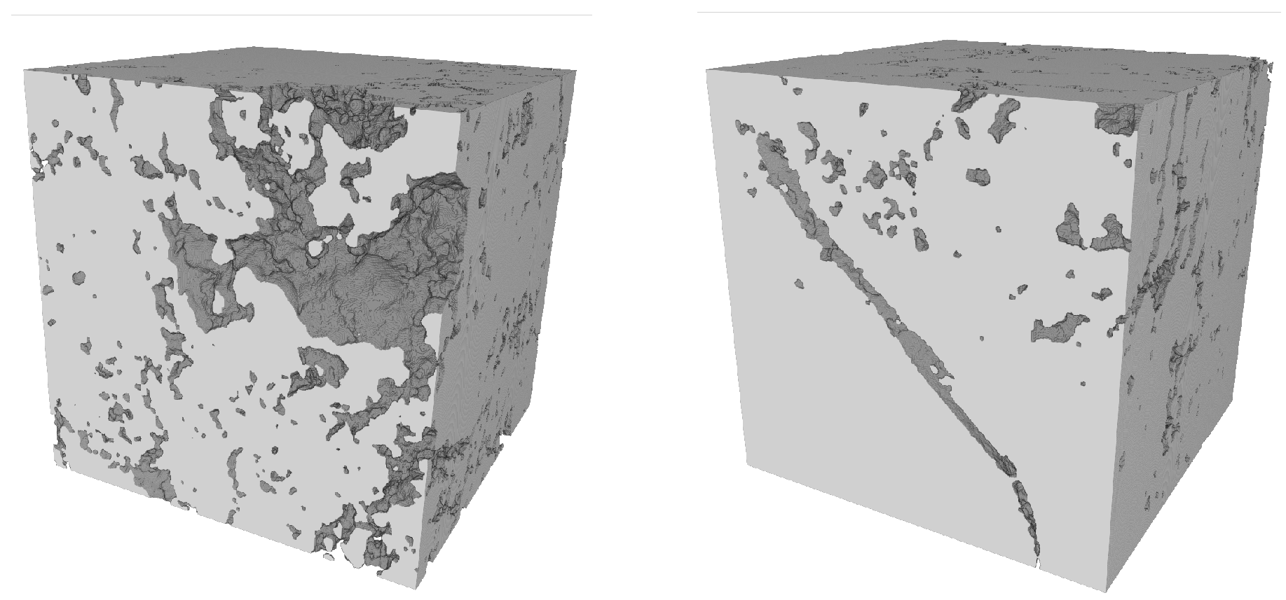
X-Ray CT (images in this study were obtained using model HMX 225 manufactured by XTek systems Ltd., UK) has proven a powerful tool to characterise pore geometry (Figure 1) at scales relevant to soil microbes with particular emphasis on bacteria [10,11] and has been used to characterize the effect of land management practices on soil architecture and subsequent microbial invasion [12,13].

Figure 1. Soil volumes quantified using X-Ray CT, gray pixels are solid, voxel resolution = 30 μm.

Figure 1. Soil volumes quantified using X-Ray CT, gray pixels are solid, voxel resolution = 30 μm.

1.3. Computational Challenges

The combination of high definition voxel data describing a soil habitat with physiologically based reaction diffusion models presents a significant challenge. The computational cost of simulating meaningful interaction between genotype (parameters governing the microbial processes) and environment is so great that conventional (scalar) programming strategies are simply not adequate. Parallelisation, in one form or another, is imperative to allow both initial exploratory investigation and subsequently to permit robust hypothesis testing (over many replicates). A typical X-Ray CT image may contain between 10⁹ and 10¹⁰ voxel elements organised as a 3D Cartesian lattice. It is common practice to select, from within the high definition volume image, a region of interest that offers a fair representation of the physical sample. Motivation in this respect is the avoidance of any artefacts or anomalies resulting from physical sampling and imaging and also the need to control the size of the data “footprint” due to the associated simulation processing cost. For example a domain size of 128 × 128 × 128 voxels has been used for the soil–microbe model (requiring data storage amounting to 300 MBytes) in order to achieve an acceptable rate of simulation. This domain size corresponds to a physical volume of approximately 0.3 cm³ at a voxel resolution of 30 microns [6] whereas for useful prediction, the broader core scale of cm³ or more may be required. This is due to the goal of verification by physical experiment which is typically carried out at the core scale. Simulations need to operate at appropriate scales in order to accurately reproduce the observed, often emergent behaviours we wish to study [14].

In the past decade, many demanding computational problems have been addressed by distributing the processing workload over a computer cluster. This offers potentially good scalability of performance versus problem size but can be costly in terms of both development effort and the necessary resource infrastructure. Given unlimited access to a sufficiently large computer cluster, a naive “brute-force” problem decomposition (e.g., many spatial sub-domains of small uniform size, each allocated to one of many computers) may be practical. More generally, however, budget constraints lead to the need for efficiency which in turn leads to increased software complexity (e.g., dynamic load balancing) and hence more costly development and maintenance. The difficulty of efficiently distributing computation for a spatially complex simulation domain such as a soil image must not, in our opinion, be under-estimated.

Contrastingly, the prospect of harnessing “the power of a cluster” within a single local computer at modest operational cost is very appealing. Contemporary graphics accelerator devices (historically often referred to as “graphics cards” or “graphics boards”) of the type marketed for playing 3D computer games on desktop computers, can be used for this purpose. Such commodity devices are available at prices ranging from under a hundred to more than a thousand euros/dollars as dictated by performance and advanced features. Over the last decade, user-programmability of these devices has improved greatly, facilitating application to problems other than the synthesis of digital images. In the mid to high end of the price range, every device consists of one or more Graphics Processing Units (henceforth GPU) supported by a very high performance memory subsystem. It is this combination of highly parallel processing unit and fast memory that offers the potential for the GPU to significantly out-perform the CPU on some types of problem. In the following section we discuss the characteristics of a typical GPU and how it may be harnessed to accelerate the simulation of soil–microbe interaction.

1.4. GPGPU

The GPU has been used extensively in non-graphical applications and is particularly well suited to operating on scalar and vector fields represented by discrete Cartesian lattices of dimension three or less, especially when the vector element count does not exceed four. The high degree of data parallelism offered by the GPU is easily exploited when computations on such a lattice are strictly localised i.e., when interaction is limited to nearest neighbour lattice sites. A class of application for which this is true, and one particularly relevant to soil ecosystem models, is the Reaction–Diffusion system. Reaction–Diffusion systems have been implemented on GPU for procedural texture generation, pollution dispersal and phase separation [15,16,17].

An added benefit of GPU-based computation is the relative ease and efficiency with which the graphics accelerator may be used to visualise the simulation as it progresses, permitting real-time interactive visual simulation. The complexity of Reaction–Diffusion systems constrained in structured soil environments make the model output difficult to comprehend and as such visualization has been proposed as a complementary approach to analysing and interpreting such data. Visual representations of simulated soil–microbe dynamics allow possible errors to be disclosed and enhance model verification. Furthermore by implementing the visualisation directly, great flexibility is realised in the mapping of multivariate spatial data to visual representations. Such an approach can be particularly beneficial during software development, when immediacy of visual feedback can enhance workflow. Contrastingly, the use of a more generic external software application for visualising such complex data may limit both flexibility and performance.

In the following section, we introduce some concepts and terminology used within the remainder of the article. GPU computation is based on rapidly changing proprietary technologies, hence we attempt to provide an accessible and standardised view on which to base subsequent discussion.

Technical Background

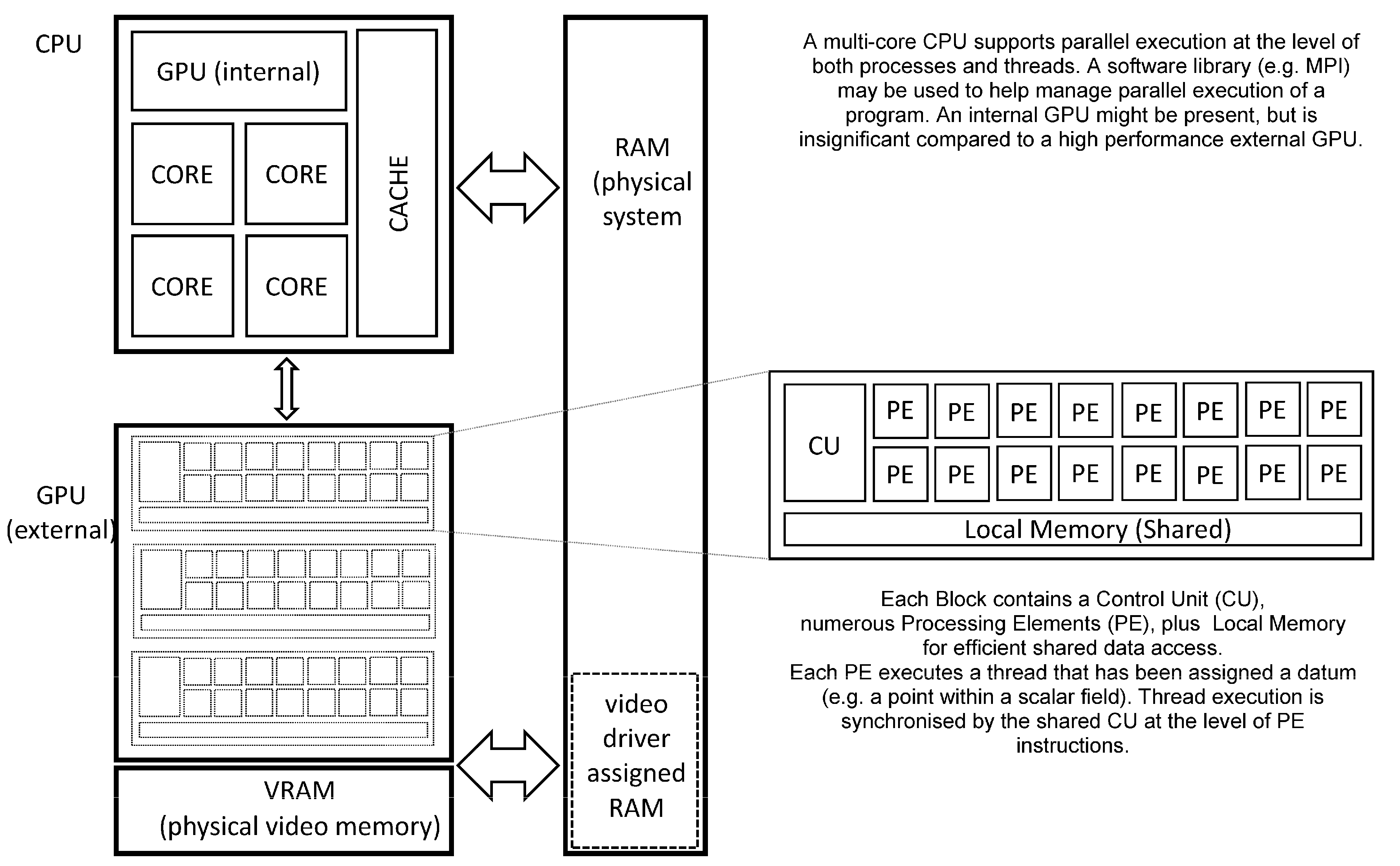
Figure 2 (below) shows the schematic organisation of a CPU and GPU within a contemporary desktop computer. The CPU provides multiple processor cores, each supporting one or more threads of a process (i.e., a program in a state of execution). Each core internally supports various forms of parallel execution via “superscalar” design features that are transparent to the program (mer). This permits high performance execution without placing a burden on software development, but greatly increases the internal complexity of each core. Cache memory is a critical feature of the CPU due to the comparatively slow RAM (Random Access Memory) that is employed as system memory. Access to the system memory is shared between all processor cores and many other devices, including the GPU.

An external high-performance GPU (in the form of a “video accelerator”) differs from the CPU by exposing parallelism to the software developer on a far greater scale. Within a single GPU there may be thousands of PE’s (Processing Elements) each executing a thread of the shader process, thus thousands of sites in a Cartesian lattice may be processed simultaneously. The PE’s are typically organised into blocks having some local memory and most importantly, a single shared CU (Control Unit) meaning that control flow is expected to be identical for all PE’s. Should control flow diverge within a PE block (i.e., conditional statements evaluate to locally different results across the block) then execution performance may suffer noticeably. The GPU is tightly coupled to video memory that offers orders of magnitude higher performance than system memory, (but may be somewhat limited in quantity due to financial considerations). This high performance video memory is critical in keeping large numbers of PE’s usefully employed without relying on a sophisticated hierarchy of cache memory (a marked contrast with the CPU). Recent generations of GPU support double precision floating point arithmetic, allowing them to be applied more easily to a wide range of scientific problems.

Communication between the CPU and GPU may be direct (e.g., changes to an internal GPU setting made by a process executing on the CPU) whereas application data is transferred using buffers allocated within system memory. Direct (synchronous) communication expends processing capacity for both CPU and GPU whereas buffered (asynchronous) communication is mainly limited by system memory performance. In order to maximise the throughput of an application, it is advisable to reduce CPU-GPU communication as far as possible, especially regarding large application data which should be transferred only when absolutely necessary.

Figure 2. Overview of GPU and CPU organization.

Figure 2. Overview of GPU and CPU organization.

In this paper we present the application of GPGPU technologies for computation and visualisation to an existing model of soil–fungi dynamics to extend the spatial scales of the computational domain, to speed up the computation and to aid in understanding and communication of system studied through tight coupling of the simulation and visualisation. Results of the GPGPU implementation were collected for single and double precision (declared as float and double in the C language family). The success of the parallelised version was assessed in terms of computation time and also the accuracy of results. We conclude with a performance evaluation to evaluate the effectiveness of the GPGPU implementation.

2. Materials and Methods

2.1. Serial CPU Implementation

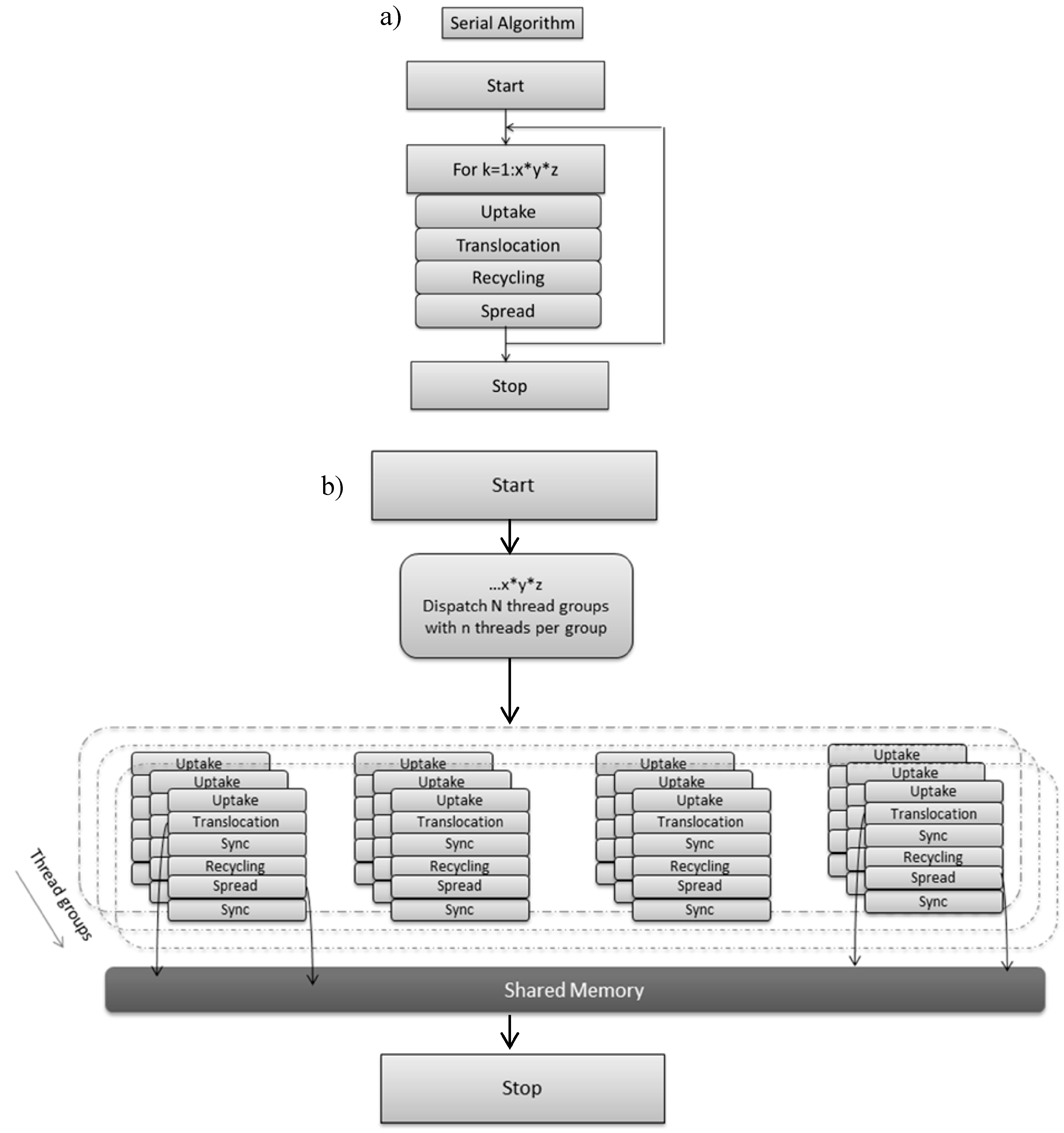
Typically reaction diffusion models are solved using a structured grid that maps to the computational domain. The model is executed on the CPU (Figure 3a) and is sequential in operation. In the non-optimized, naive CPU serial implementation 3D scalar fields with double precision are allocated and initialised that store the state variables described in Box 1. For the desired number of iterations (1000) the uptake, translocation, recycling and diffusion/spread algorithms are applied sequentially to each voxel of the 3D grid using a triple for loop and a single thread/process (Figure 3a). The duration of the simulation is determined by the time the biomass approaches the simulation boundaries (1000 iterations). Double buffering is applied to maintain data integrity. Compute time is up to 6 min with double precision. The serial version was run on the following hardware 16GB RAM and Intel (g) Xeon (R) CPU E3.

Figure 3. (a) Serial CPU version of soil–fungal dynamic; (b) GPU implementation of soil–fungal dynamic decomposed into thread groups with each thread group accessing shared memory and upon which access to threads are synchronised.

Figure 3. (a) Serial CPU version of soil–fungal dynamic; (b) GPU implementation of soil–fungal dynamic decomposed into thread groups with each thread group accessing shared memory and upon which access to threads are synchronised.

2.2. GPU Implementation

Grid based computation maps well to GPUs and the state variables (Box 1) are implemented as numeric data within a grid cell, and the algorithm steps are the computational kernels or shaders operating on grid cell data. The DirectX API (Application Programming Interfaces) is known to offer efficient inter-operability with computation and graphics and was selected for this reason, as immediacy of visual feedback was a key objective, together with familiarity of the API via 3D graphics programming [18]. A thread executing shader code is invoked for each grid cell, thus the total number of such invocations per iteration (and per shader) is equal to the number of voxels in the 3D spatial domain. Figure 3b outlines how parallel computations can accelerate soil–microbe dynamics. In the parallel approach the computations are distributed across thread groups, and threads within a thread group execute concurrently. Thread Group Shared Memory is an efficient local storage feature, useful for sharing intermediate calculations between neighbouring grid cells. Thread synchronization is required immediately after loading data to shared memory to ensure data integrity. The number of threads per group is context dependent and a scalability study is required to determine the optimal arrangement [18].The author of [18] suggests that, due to the graphics hardware, threads in a group should be a multiple of 32, and that 128 threads per group is a reasonable starting point for scalability analysis.

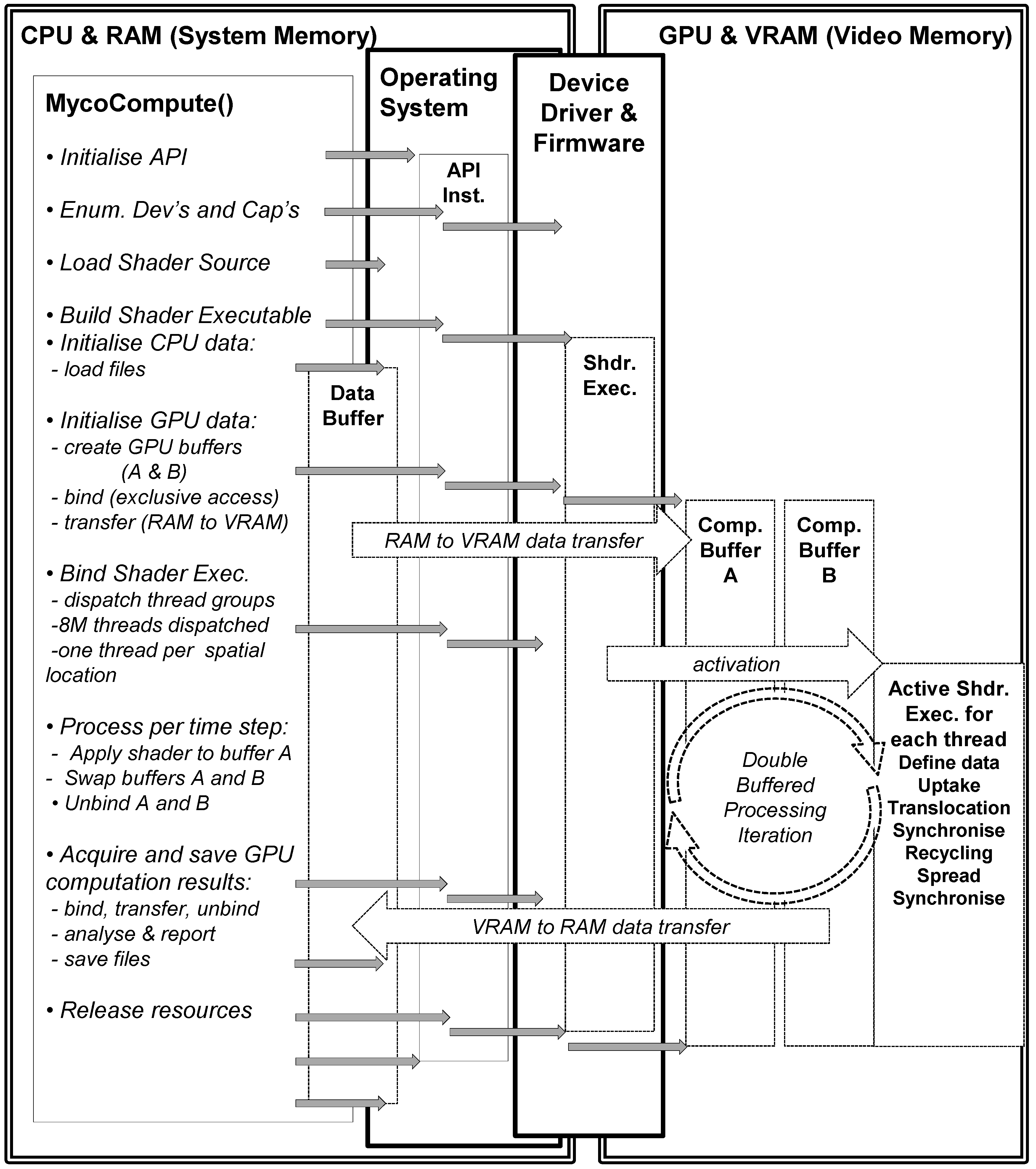
For the GPU implementation the sequence of operations (Figure 4) includes firstly initialising the graphics and computation API (DirectX 11), and secondly verifying the capabilities of the graphics card (some may not support compute functionality, double precision or even basic floating point operations). Next the shader source code is compiled for the graphics card and the data buffers (the 3D scalar fields of Box 1) in RAM are initialised by the CPU. Once the GPU buffers have been both defined and activated, then the contents of these buffers are transferred from RAM to VRAM (Video RAM). The data accessed by a shader thread executing on the GPU is defined in the form of a 1D unstructured buffer in VRAM, but this usage is semantically identical to that of the 3D scalar field located in RAM. The data is subsequently activated (bound) to the GPU pipeline awaiting an activated/bound shader to operate on the data.

The appropriate shader/kernel (computation or rendering) is also activated (bound) and the shader will operate on the currently activated data either for computation or rendering. The compute shader is invoked for each thread which uses an index to map into the data stream and applies the uptake, translocation, recycling and spread calculations. Synchronisation is necessary in the translocation and spread processes as diffusion is implemented to ensure all threads in a group reach a certain state before proceeding with the other reaction functions (uptake, translocation and recycling). The application of the shader to the numeric data within a grid cell generates updated numeric data which becomes the input to the next step. This cyclic process is illustrated in right hand side of Figure 4—GPU and VRAM section. Periodically data is transferred from GPU to CPU to test for mass conservation. The compute shader is deactivated and the rendering shader is activated together with the data it requires for rendering the result of the computation. The rendering uses the result of the compute shader as input, the 1d unstructured buffer is copied into a 3D texture where the three biomass types are mapped to r, g, b channels of a 3D texture. The parallel version was run using the following hardware (NVIDIA GeForce GTX 650 Ti with 1024 MB VRAM, Nvidia, Santa Clara, CA, USA).

Figure 4. Sequence of events for GPU computation of soil–microbe model.

Figure 4. Sequence of events for GPU computation of soil–microbe model.

3. Results and Discussion

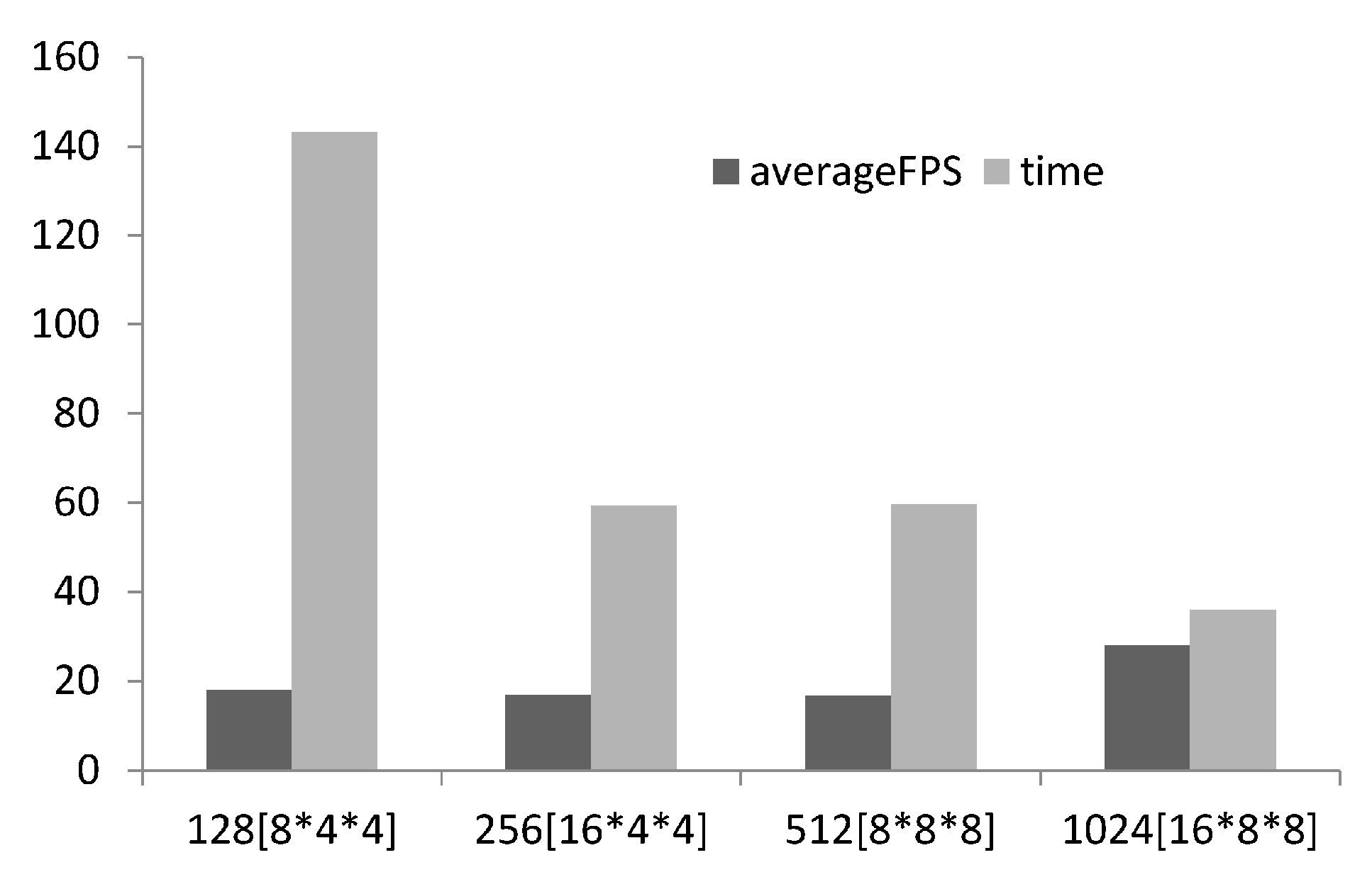
Scalability analysis was conducted investigating the effect of thread group size on time to compute and the frames rendered per second. For structured grid problems like Reaction–Diffusion problems the number of threads required is known, equal to the number of voxels in the computational domain, but how many threads to allocate per group should be tuneable and determined on a case by case basis via scalability analysis [17,19] (illustrated in Figure 5). As suggested by [17] 128 threads per group was used for the lower limit and incremented by 256 up to the maximum number of threads per group (1028). The number of threads allocated was a multiple of the warp size (32 for NVIDEA hardware). With increasing threads per group better performance is achieved, this may seem obvious but it is recommended to undertake the scalability analysis as it is not always the case. 1028 threads per group was selected for the study.

Figure 5. Bar chart showing scalability analysis of # threads per group, the thread group topology is presented in square brackets, on FPS and time to compute.

Figure 5. Bar chart showing scalability analysis of # threads per group, the thread group topology is presented in square brackets, on FPS and time to compute.

The cost of data movement from GPU to CPU, and rendering the simulation output was investigated by determining the compute time with increasing frequency of data transfer and the draw frequency. Table 1 shows the time to compute and frames per second (fps) based on draw rate and data transfer from GPU to CPU frequency. The time to compute accounts for all the CPU and GPU run time for the GPU results which include memory transfer time between CPU and GPU as a function of transfer frequency. The results highlights that resources used for rendering is negligible and is reflected in the simplicity of the renderer. Transferring data from CPU to GPU is costly effecting both time to compute and fps and should be done minimally.

Table 1. Time elapsed and fps as a function of draw rate and data transfer from GPU to CPU for single precision.

Draw Rate	50	50	50	10	1
GPU → CPU	50	10	1	50	50
FPS	24	24	6	24	24
Time elapsed(s)	50.85	57.96	143.12	50.8	55.98

Table 1. Time elapsed and fps as a function of draw rate and data transfer from GPU to CPU for single precision.

Draw Rate	50	50	50	10	1
GPU → CPU	50	10	1	50	50
FPS	24	24	6	24	24
Time elapsed(s)	50.85	57.96	143.12	50.8	55.98

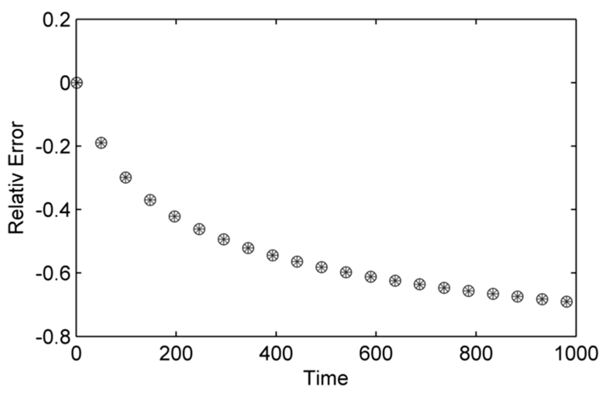
Results collected focus on the accuracy of the GPU implementations measured by relative error with respect to the CPU implementation being the true value and the GPU (float and double) being approximated values (Figure 6). Figure 6 shows little difference between single and double precision in terms of solution accuracy of numerical scheme recovering the conservation of mass. The relative error increases with time as its cumulative and plateaus as no more calculations are conducted as the simulation is space limited; this may have consequences for running longer term simulations when the computational domain is larger and is replenished as the error will continue to grow. Figure 7 depicts time to compute (n = 5) and highlights the difference between GPU implementations. The figure shows that the GPU single precision was fastest followed by double precision. 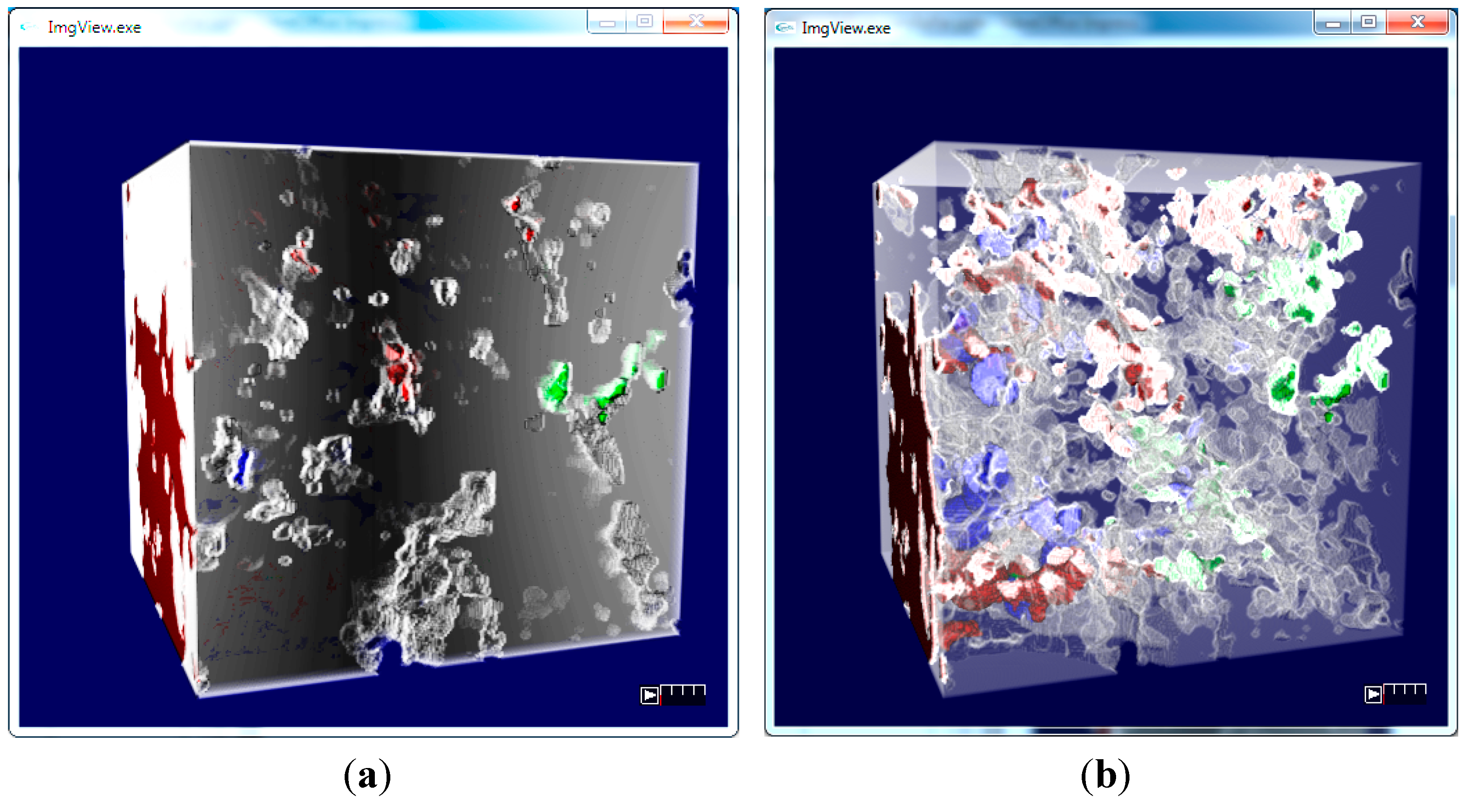Figure 8 shows the rendered simulation output which is displayed in real-time, which can be queried as the simulation proceeds, providing the immediacy in visual feedback as required.

Figure 6. Relative error for the GPU implementation with single (open circles) and double precision (stars).

Figure 6. Relative error for the GPU implementation with single (open circles) and double precision (stars).

Figure 7. Time elapsed (n = 5) for GPU versions for a simulation with 1000 iterations.

Figure 7. Time elapsed (n = 5) for GPU versions for a simulation with 1000 iterations.

Figure 8. (a) Microbial biomass growing in the soil structure; (b) view of the soil pore volume together with the distribution of the types of biomass—green is NIB, red is IR and blue is IN biomass. The dominant biomass type is displayed per voxel.

Figure 8. (a) Microbial biomass growing in the soil structure; (b) view of the soil pore volume together with the distribution of the types of biomass—green is NIB, red is IR and blue is IN biomass. The dominant biomass type is displayed per voxel.

4. Conclusions

The paper set out to present the stages for porting a serial CPU-based Reaction–Diffusion model to the GPU. The software required to perform general set-up, loading resource files, etc., is much the same in either case, but there is additional initialisation and management required in the case of the GPU. The transformation of CPU based Reaction–Diffusion simulation code into a GPU compute kernel is not difficult and, by liberating the simulation model from the “baggage” of explicit nested iteration, tends to clarify and highlight the essential features of a model implementation. Contrasting with this is the effort required to set up the infrastructure necessary for compute kernel execution, which is more challenging and has a steep learning curve. The results are promising in terms of computational performance, showing a 21 times speedup relative to the single threaded CPU model reference point, following some limited tuning of GPU data handling i.e., transferring data between CPU and GPU less frequently. This speed up is still achieved while simultaneously presenting approximately 30 fps interactive 3D visualisation of simulation output that is captured at intervals of 50 iterations. We emphasise that this visualisation uses only the simplest 3D rendering techniques so as not to impact noticeably on system performance. Nonetheless, the ability to directly observe the simulation evolving is extremely helpful for understanding the interplay of the state variables in a spatially complex environment such as soil.

In terms of increasing spatial scale, a GPU implementation improves practicality by significantly reducing the burden of computation time, but is intrinsically limited by the quantity of video memory provided within the GPU device (typically 2 to 4 GBytes for commodity devices at the time of writing). Consequently very large spatial domains must be distributed across multiple GPUs such that communication via the relatively slow system memory does not become a limiting factor. Such distribution must be explicitly managed by the application, a non-trivial task that has not been addressed within the present study. With respect to accuracy and robustness of the translation to GPU computation, differences between single and double precision were not apparent over the time scales and model conditions assessed. Under these conditions, the results of GPU simulation compared well with those of the CPU but we stress that one cannot expect the output from such different devices to match exactly. Despite improving compliance with the widely accepted IEEE-754 standard [20] for floating point arithmetic, the ordering of machine instructions can affect numerical evaluation through truncation and rounding of intermediate results. Just as different compilers and optimisation settings may produce slightly different results on a single CPU, the translation of a compute kernel into GPU executable code provides no guarantees of end-to-end precision over a complex calculation. As this translation is implemented within GPU device driver software, it is proprietary to the GPU manufacturer and may be subject to change in the event that device drivers are updated. Further issues may stem from the API layer acting as intermediary between the application and the drivers, e.g., DirectCompute is known to presently restrict floating point division operations to single precision and does not support FMA (Fused Multiply Add) instructions. These are factors that may contribute to the lack of clear differences between single and double precision implementations.

The Microsoft Direct3D API was selected based on previous experience in 3D image synthesis, but this familiarity was perhaps not the best motivation. For many reasons including control over precision, scalability, quality of documentation and availability of community support, other API’s such as OpenCL (Open Computing Language) and CUDA (Compute Unified Device Architecture) may have be more appropriate choices. Despite such issues, the performance improvement realised for intermediate spatial scales has been rewarding in itself as the scope of simulation experiments, i.e., the capability to investigate a wider range of model parameters, is now significantly enhanced. This is a key aspect of the application to environmental research, in which we seek to understand the interaction between genotype trait and habitat under a wide range of environmental conditions.

References

- Clemmensen, K.E.; Bahr, A.; Ovaskainen, O.; Dahlberg, A.; Ekblad, A.; Wallander, H.; Stenlid, J.; Finlay, R.D.; Wardle, D.A.; Lindahl, B.D. Roots and associated fungi drive long-term carbon sequestration in boreal forest. Science 2013, 339, 1615–1618. [Google Scholar] [CrossRef] [PubMed]
- Falconer, R.E.; Bown, J.L.; White, N.A.; Crawford, J.W. Biomass recycling and the origin of phenotype in fungal mycelia. Proc. Biol. Sci. 2005, 272, 1727–1734. [Google Scholar] [CrossRef] [PubMed]
- Cazelles, K.; Otten, W.; Baveye, P.C.; Falconer, R.E. Soil fungal dynamics: Parameterisation and sensitivity analysis of modelled physiological processes, soil architecture and carbon distribution. Ecol. Modell. 2013, 248, 165–173. [Google Scholar] [CrossRef]
- Falconer, R.E.; Houston, A.; Otten, W.; Baveye, P.C. Emergent Behavior of Soil Fungal Dynamics: Influence of Soi. J. Soil Sci. 2012, 177, 111–119. [Google Scholar] [CrossRef]
- Falconer, R.E.; Bown, J.L.; White, N.A.; Crawford, J.W. Biomass recycling: A key to efficient foraging by fungal colonies. Oikos 2007, 116, 1558–1568. [Google Scholar] [CrossRef]
- Manzoni, S.; Porporato, A. Soil carbon and nitrogen mineralization: Theory and models across scales. Soil Biol. Biochem. 2009, 41, 1355–1379. [Google Scholar] [CrossRef]
- Dungait, J.A.J.; Hopkins, D.W.; Gregory, A.S.; Whitmore, A.P. Soil organic matter turnover is governed by accessibility not recalcitrance. Glob. Chang. Biol. 2012, 18, 1781–1796. [Google Scholar] [CrossRef]
- Otten, W.; Pajor, R.; Schmidt, S.; Baveye, P.C.; Hague, R.; Falconer, R.E. Combining X-Ray CT and 3D printing technology to produce microcosms with replicable, complex pore geometries. Soil Biol. Biochem. 2012, 51, 53–55. [Google Scholar] [CrossRef]
- Crawford, J.W.; Deacon, L.; Grinev, D.; Harris, J.A.; Ritz, K.; Singh, B.K.; Young, I. Microbial diversity affects self-organization of the soil-microbe system with consequences for function. J. R. Soc. Interface 2012, 9, 1302–1310. [Google Scholar] [CrossRef] [PubMed]
- Wolf, A.B.; Vos, M.; de Boer, W.; Kowalchuk, G.A. Impact of matric potential and pore size distribution on growth dynamics of filamentous and non-filamentous soil bacteria. PLoS One 2013, 8, e83661. [Google Scholar] [CrossRef] [PubMed]
- Raynaud, X.; Nunan, N. Spatial ecology of bacteria at the microscale in soil. PLoS One 2014, 9, e87217. [Google Scholar] [CrossRef] [PubMed]
- Pajor, R.; Falconer, R.; Hapca, S.; Otten, W. Modelling and quantifying the effect of heterogeneity in soil physical conditions on fungal growth. Biogeosci. Discuss. 2010, 7, 3477–3501. [Google Scholar] [CrossRef]
- Kravchenko, A.; Falconer, R.E.; Grinev, D.; Otten, W. Fungal colonization in soils with different management histories: Modeling growth in three-dimensional pore volumes. Ecol. Appl. 2011, 21, 1202–1210. [Google Scholar] [CrossRef] [PubMed]
- Falconer, R.E.; Bown, J.L.; McAdam, E.; Perez-Reche, P.; Sampson, A.T.; van den Bulcke, J.; White, N.A. Modelling fungal colonies and communities: Challenges and opportunities. IMA Fungus 2010, 1, 155–159. [Google Scholar] [CrossRef] [PubMed]
- Molnár, F.; Izsák, F.; Mészáros, R.; Lagzi, I. Simulation of reaction–diffusion processes in three dimensions using CUDA. Chemom. Intell. Lab. Syst. 2011, 108, 76–85. [Google Scholar] [CrossRef]
- Richmond, P.; Walker, D.; Coakley, S.; Romano, D. High performance cellular level agent-based simulation with FLAME for the GPU. Brief. Bioinform. 2010, 11, 334–347. [Google Scholar] [CrossRef] [PubMed]
- Sanderson, A.R.; Meyer, M.D.; Kirby, R.M.; Johnson, C.R. A framework for exploring numerical solutions of advection–reaction–diffusion equations using a GPU-based approach. Comput. Vis. Sci. 2008, 12, 155–170. [Google Scholar] [CrossRef]
- Fung, J. DirectCompute Lecture Series 210: GPU Optimizations and Performance. Available online: http://channel9.msdn.com/Blogs/gclassy/DirectCompute-Lecture-Series-210-GPU-Optimizations-and-Performance (accessed on 2 February 2015).
- NVIDIA Corporation; Harris, M. Mapping Computational Concepts to GPUs. In GPU Gems 2: Programming Techniques for High-Performance Graphics and General-Purpose Computation, 1st ed.; Fernando, M., Pharr, R., Eds.; Addison Wesley: Boston, MA, USA, 2005. [Google Scholar]
- Whitehead, N.; Fit-Florea, A. Precision & Performance: Floating Point and IEEE 754 Compliance for NVIDIA GPUs; Technical Report, rn (A+ B) 21 (2011) 1-1874919424; NVIDIA: Santa Clara, CA, USA, 2011. [Google Scholar]
© 2015 by the authors; licensee MDPI, Basel, Switzerland. This article is an open access article distributed under the terms and conditions of the Creative Commons Attribution license (http://creativecommons.org/licenses/by/4.0/).