
Computational Approach to 3D Modeling of the Lymph Node Geometry


Abstract
:
1. Introduction
2. Materials and Methods


3. Results and Discussion
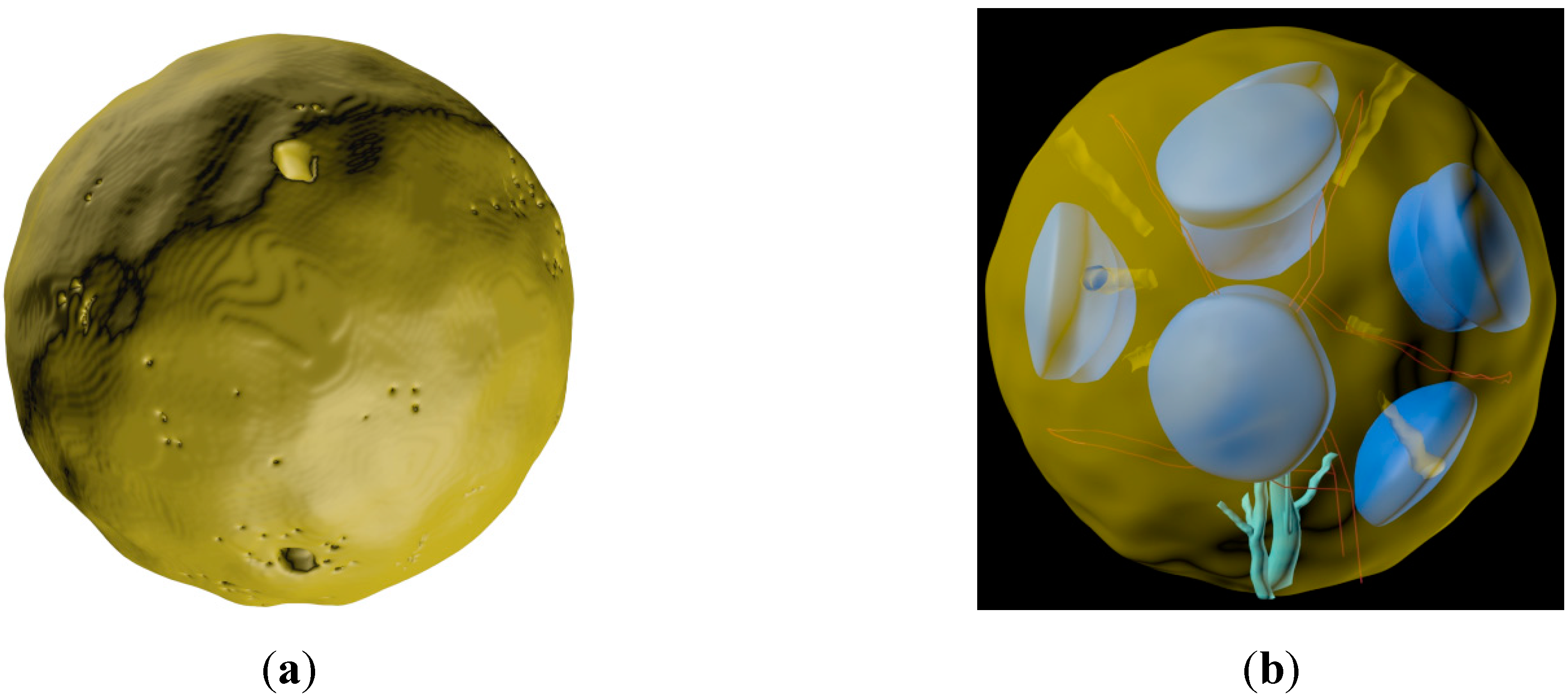
3.1. B Cell Follicles, Trabecular Sinuses, Blood Vessels and Medulla
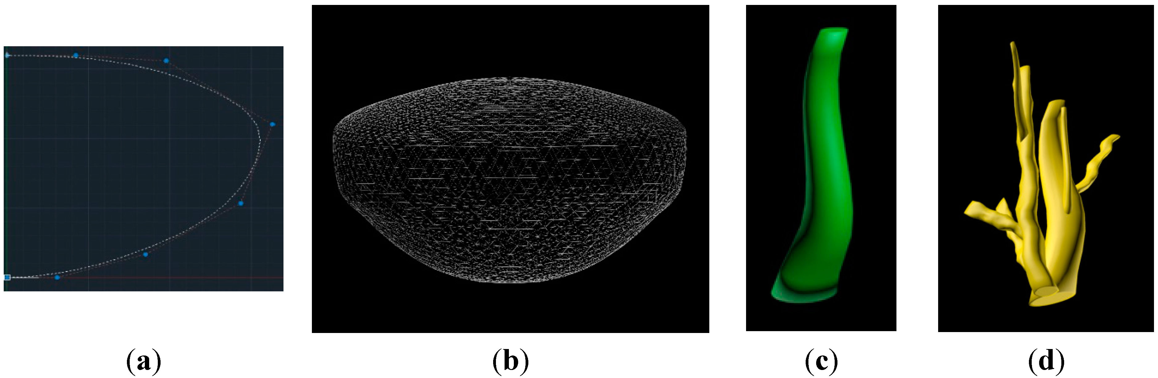
- (1)
- Initial piecewise-linear approximation of the B cell follicle border is created by marking several points on the confocal image.
- (2)
- Smoothing of the 2D object using spline approximation.
- (3)
- Generating an updated set of the border points.
- (4)
- Setting up the number of triangles on the surface of the object to achieve a required mesh resolution to be used for computational discretization of the B cell follicle.


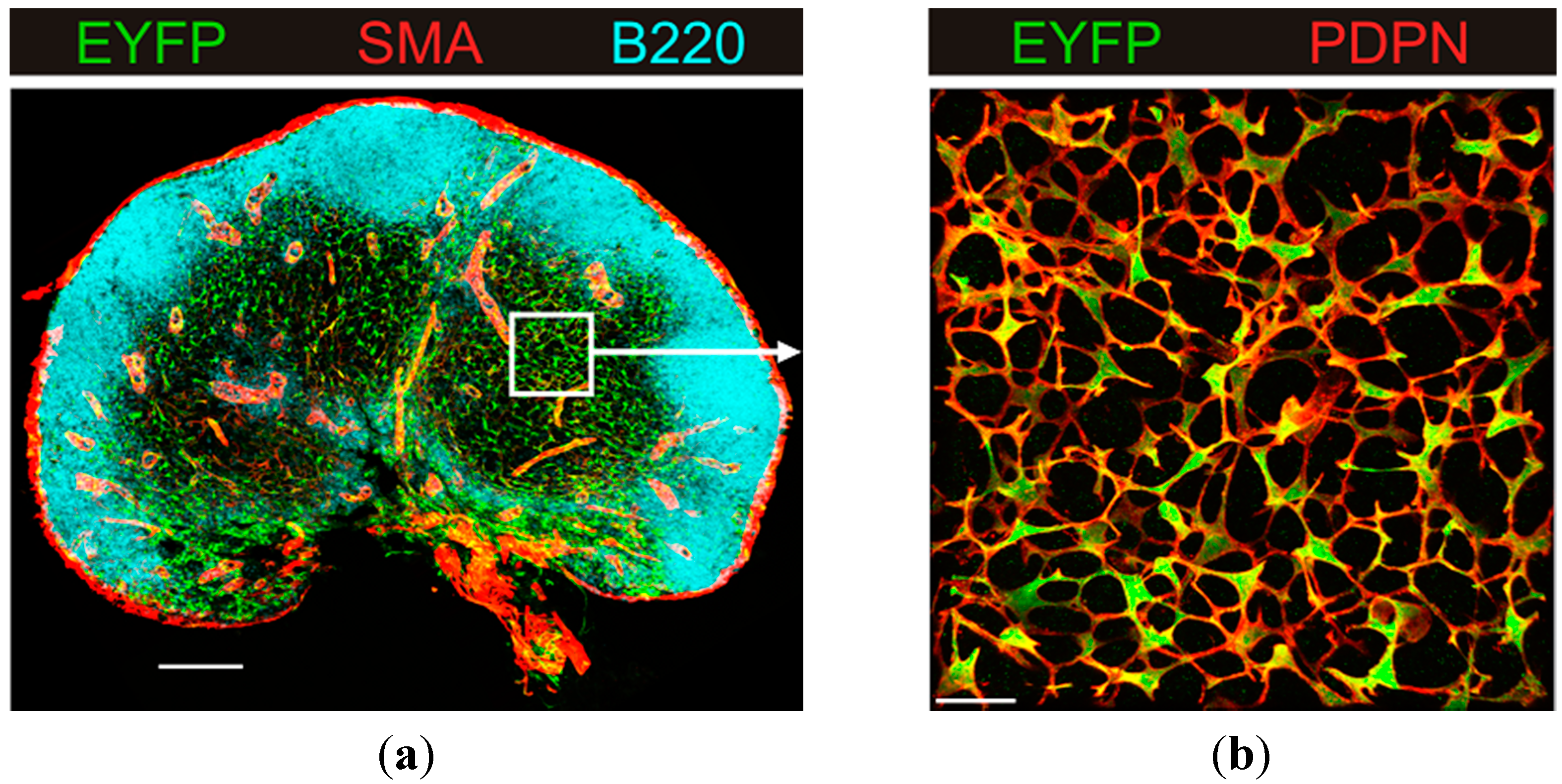
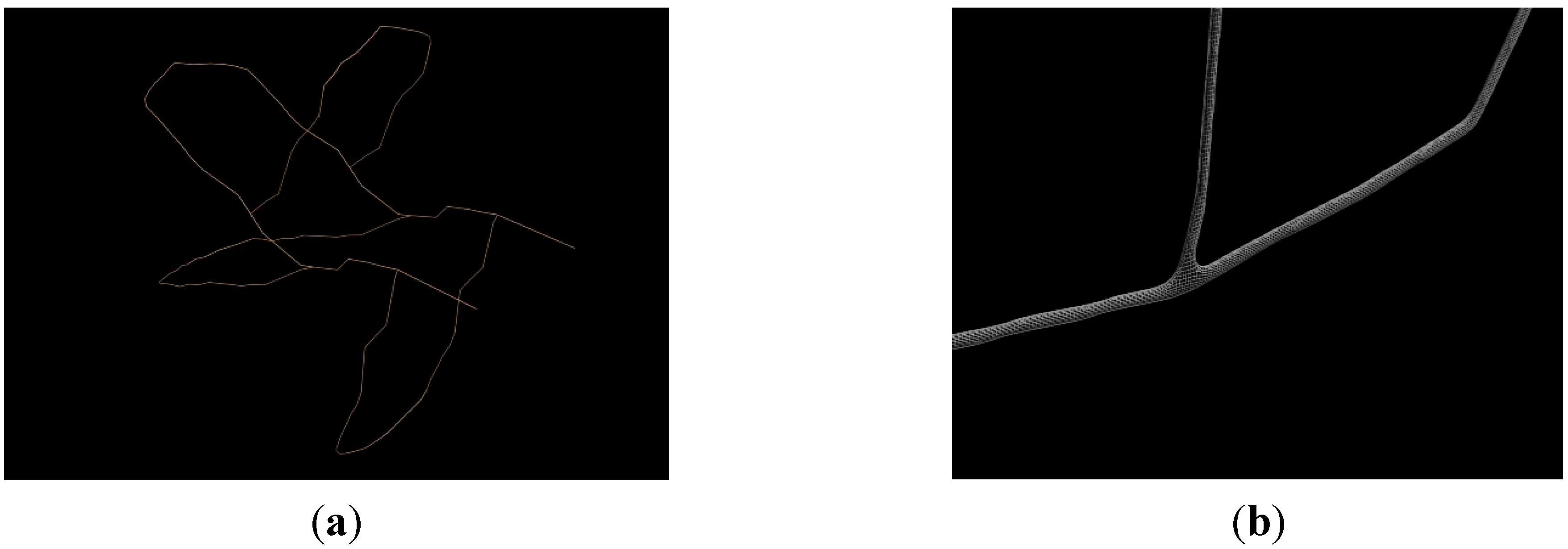
3.2. Generation of the FRC Network
- (1)
- Generate the FRC network tree according to the experimental statistical data.
- (2)
- Build the voxel approximation according to the FRC network tree.
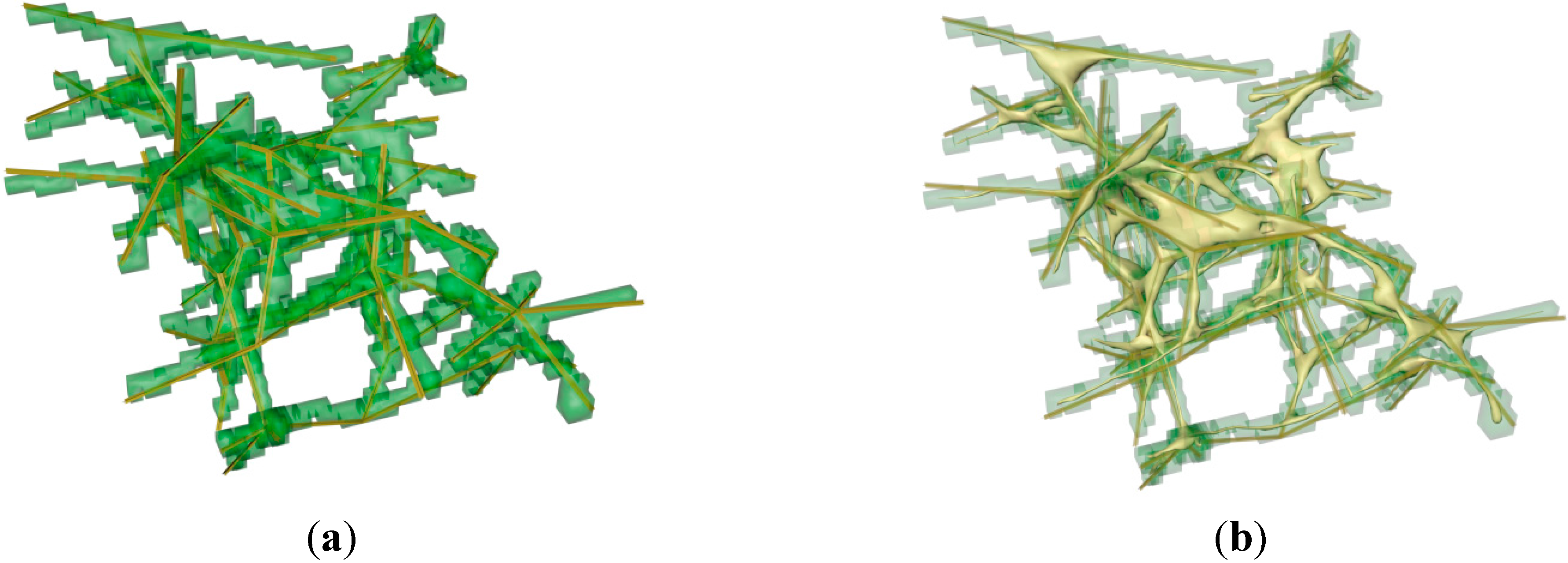
- (3)
- Cut intersecting segments of FRC voxel approximation.
- (4)
- Cut separated voxels.
- (5)
- Convert the voxel approximation to triangulated surface mesh.
- (6)
- Smooth the triangulation and export the solid object as an OBJ model.

| Name | Description | Value |
|---|---|---|
| possErr | Acceptable error length for node group of edge vectors | 0.4 |
| minDist | Minimal possible distance between two nodes of the FRC tree | 11.0 |
| voxLength | Dimension of voxel cube, µm | 2.0 |
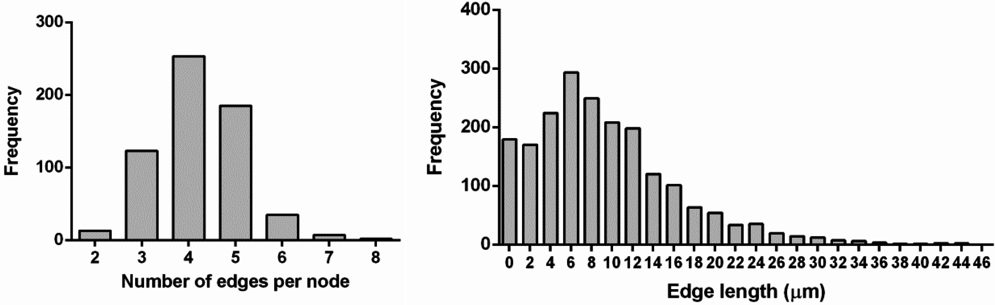
| nodeLength | Statistic data on edge length, µm | 0.24–44.73 |
| (mean value 11.63) | ||
| See also Figure 2 | ||
| nodePipes | Experimental data on the node edges count | 2–7 (mean square 4.22) |
| See also Figure 2 |

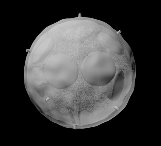
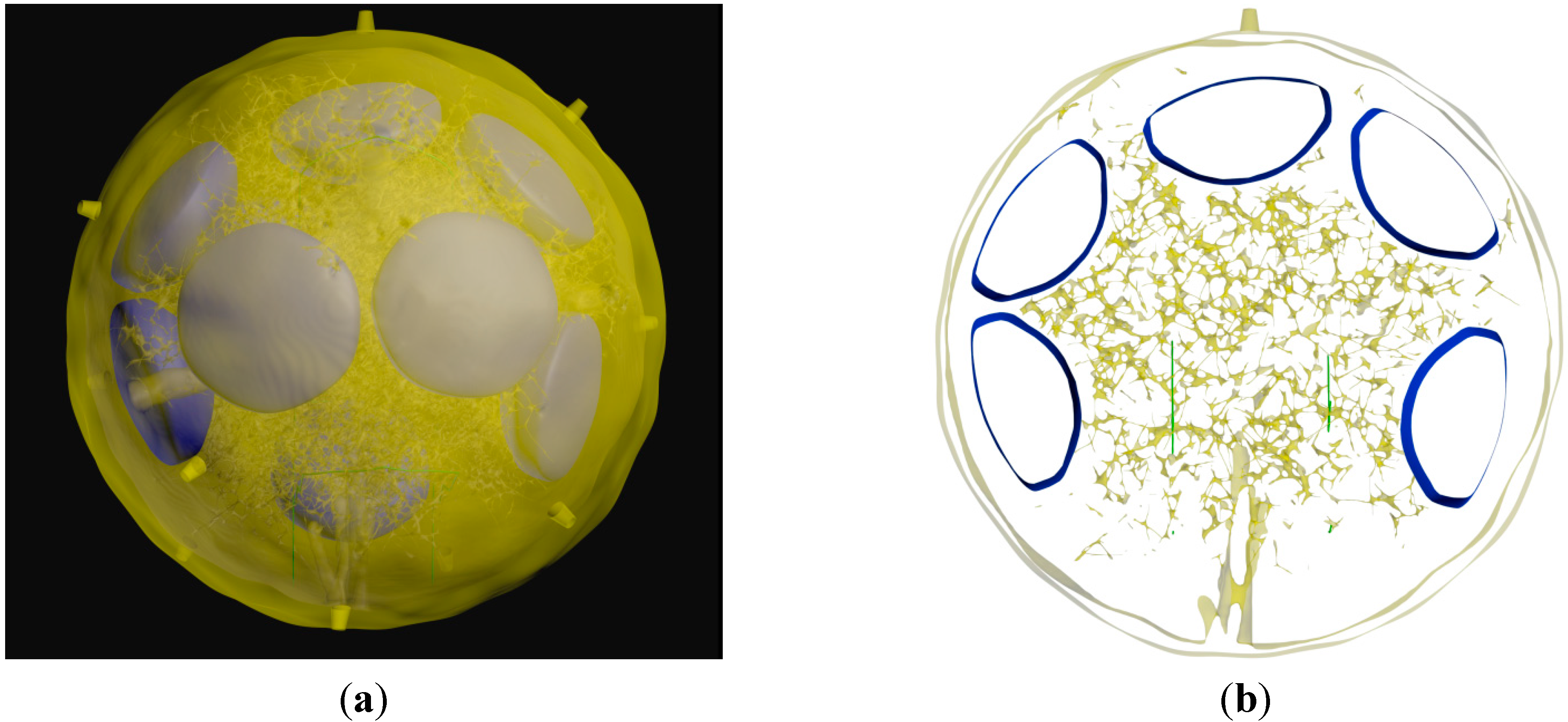
3.3. Generation of the Whole LN


4. Conclusions
Supplementary Information
Acknowledgments
Author Contributions
Conflicts of Interest
References
- Ludewig, B.; Stein, J.V.; Sharpe, J.; Cervantes-Barragan, L.; Thiel, V.; Bocharov, G. A global “imaging” view on systems approaches in immunology. Eur. J. Immunol. 2012, 42, 3116–3125. [Google Scholar] [CrossRef] [PubMed]
- Gretz, J.E.; Anderson, A.O.; Shaw, S. Cords, channels, corridors and conduits: Critical architectural elements facilitating cell interactions in the lymph node cortex. Immunol. Rev. 1997, 156, 11–24. [Google Scholar] [CrossRef] [PubMed]
- Willard-Mack, C.L. Normal structure, function, and histology of lymph nodes. Toxicol. Pathol. 2006, 34, 409–424. [Google Scholar] [CrossRef] [PubMed]
- Junt, T.; Scandella, E.; Ludewig, B. Form follows function: Lymphoid tissue microarchitecture in antimicrobial immune defence. Nat. Rev. Immunol. 2008, 8, 764–775. [Google Scholar] [CrossRef] [PubMed]
- Girard, J.P.; Moussion, C.; Förster, R. HEVs, lymphatics and homeostatic immune cell trafficking in lymph nodes. Nat. Rev. Immunol. 2012, 12, 762–773. [Google Scholar] [CrossRef] [PubMed]
- Malhotra, D.; Fletcher, A.L.; Turley, S.J. Stromal and hematopoietic cells in secondary lymphoid organs: Partners in immunity. Immunol. Rev. 2013, 251, 160–176. [Google Scholar] [CrossRef] [PubMed]
- Mueller, S.N.; Germain, R.N. Stromal cell contributions to the homeostasis and functionality of the immune system. Nat. Rev. Immunol. 2009, 9, 618–629. [Google Scholar] [PubMed]
- Margaris, K.N.; Black, R.A. Modelling the lymphatic system: Challenges and opportunities. J. R. Soc. Interface 2012, 9, 601–612. [Google Scholar] [CrossRef] [PubMed]
- Baldazzi, V.; Paci, P.; Bernaschi, M.; Castiglione, F. Modeling lymphocyte homing and encounters in lymph nodes. BMC Bioinform. 2009, 10, 387. [Google Scholar] [CrossRef]
- Bogle, G.; Dunbar, P.R. On-lattice simulation of T cell motility, chemotaxis, and trafficking in the lymph node paracortex. PLoS ONE 2012, 7, e45258. [Google Scholar] [CrossRef] [PubMed]
- Graw, F.; Regoes, R.R. Influence of the fibroblastic reticular network on cell-cell interactions in lymphoid organs. PLoS Comput. Biol. 2012, 8, e1002436. [Google Scholar] [CrossRef] [PubMed]
- Gong, C.; Mattila, J.T.; Miller, M.; Flynn, J.L.; Linderman, J.J.; Kirschner, D. Predicting lymph node output efficiency using systems biology. J. Theor. Biol. 2013, 335, 169–184. [Google Scholar] [CrossRef] [PubMed]
- Mirsky, H.P.; Miller, M.J.; Linderman, J.J.; Kirschner, D.E. Systems biology approaches for understanding cellular mechanisms of immunity in lymph nodes during infection. J. Theor. Biol. 2011, 287, 160–170. [Google Scholar] [CrossRef] [PubMed]
- Prokopiou, S.A.; Barbarroux, L.; Bernard, S.; Mafille, J.; Leverrier, Y.; Arpin, C.; Marvel, J.; Gandrillon, O.; Crauste, F. Multiscale Modeling of the Early CD8 T-Cell Immune Response in Lymph Nodes: An Integrative Study. Computation 2014, 2, 159–181. [Google Scholar] [CrossRef]
- Bocharov, G.; Danilov, A.; Vassilevski, Y.; Marchuk, G.I.; Chereshnev, V.A.; Ludewig, B. Reaction-Diffusion Modelling of Interferon Distribution in Secondary Lymphoid Organs. Math. Model. Nat. Phenom. 2011, 6, 13–26. [Google Scholar] [CrossRef]
- Grigorova, I.L.; Panteleev, M.; Cyster, J.G. Lymph node cortical sinus organization and relationship to lymphocyte egress dynamics and antigen exposure. Proc. Natl. Acad. Sci. USA 2010, 107, 20447–20452. [Google Scholar] [CrossRef] [PubMed]
- Kumar, V.; Scandella, E.; Danuser, R.; Onder, L.; Nitschké, M.; Fukui, Y.; Halin, C.; Ludewig, B.; Stein, J.V. Global lymphoid tissue remodeling during a viral infection is orchestrated by a B cell-lymphotoxin-dependent pathway. Blood 2010, 115, 4725–4733. [Google Scholar] [CrossRef] [PubMed]
- Textor, J.; Peixoto, A.; Henrickson, S.E.; Sinn, M.; von Andrian, U.H.; Westermann, J. Defining the quantitative limits of intravital two-photon lymphocyte tracking. Proc. Natl. Acad. Sci. USA 2011, 108, 12401–12406. [Google Scholar] [CrossRef] [PubMed]
- Textor, J.; Henrickson, S.E.; Mandl, J.N.; von Andrian, U.H.; Westermann, J.; de Boer, R.J.; Beltman, J.B. Random migration and signal integration promote rapid and robust T cell recruitment. PLoS Comput. Biol. 2014, 10, e1003752. [Google Scholar] [CrossRef] [PubMed]
- Irla, M.; Guenot, J.; Sealy, G.; Reith, W.; Imhof, B.A.; Sergé, A. Three-dimensional visualization of the mouse thymus organization in health and immunodeficiency. J. Immunol. 2013, 190, 586–596. [Google Scholar] [CrossRef] [PubMed]
- Beltman, J.B.; Marée, A.F.; Lynch, J.N.; Miller, M.J.; de Boer, R.J. Lymph node topology dictates T cell migration behavior. J. Exp. Med. 2007, 204, 771–780. [Google Scholar] [CrossRef] [PubMed]
- Bajénoff, M.; Egen, J.G.; Koo, L.Y.; Laugier, J.P.; Brau, F.; Glaichenhaus, N.; Germain, R.N. Stromal cell networks regulate lymphocyte entry, migration, and territoriality in lymph nodes. Immunity 2006, 25, 989–1001. [Google Scholar] [CrossRef] [PubMed]
- Donovan, G.M.; Lythe, G. T-cell movement on the reticular network. J. Theor. Biol. 2012, 295, 59–67. [Google Scholar] [CrossRef] [PubMed]
- Klauschen, F.; Qi, H.; Egen, J.G.; Germain, R.N.; Meier-Schellersheim, M. Computational reconstruction of cell and tissue surfaces for modeling and data analysis. Nat. Protoc. 2009, 4, 1006–1012. [Google Scholar] [CrossRef] [PubMed]
- Chai, Q.; Onder, L.; Scandella, E.; Gil-Cruz, C.; Perez-Shibayama, C.; Cupovic, J.; Danuser, R.; Sparwasser, T.; Luther, S.A.; Thiel, V.; Rülicke, T.; Stein, J.V.; Hehlgans, T.; Ludewig, B. Maturation of lymph node fibroblastic reticular cells from myofibroblastic precursors is critical for antiviral immunity. Immunity 2013, 38, 1013–1024. [Google Scholar] [CrossRef] [PubMed]
- Peters, J. Efficient one-sided linearization of spline geometry. In Mathematics of Surfaces; Wilson, W.J., Martin, R.R., Eds.; Springer-Verlag: Berlin, Germany, 2003; pp. 297–319. [Google Scholar]
- Gershenfeld, N. The Nature of Mathematical Modelling; Cambridge University Press: Cambridge, UK, 1999; p. 344. [Google Scholar]
- Fletcher, C.V.; Staskus, K.; Wietgrefe, S.W.; Rothenberger, M.; Reilly, C.; Chipman, J.G.; Beilman, G.J.; Khoruts, A.; Thorkelson, A.; Schmidt, T.E.; et al. Persistent HIV-1 replication is associated with lower antiretroviral drug concentrations in lymphatic tissues. Proc. Natl. Acad. Sci. USA 2014, 111, 2307–2312. [Google Scholar] [CrossRef] [PubMed]
- Tang, J.; van Panhuys, N.; Kastenmüller, W.; Germain, R.N. The future of immunoimaging–deeper, bigger, more precise, and definitively more colorful. Eur. J. Immunol. 2013, 43, 1407–1412. [Google Scholar] [CrossRef] [PubMed]
© 2015 by the authors; licensee MDPI, Basel, Switzerland. This article is an open access article distributed under the terms and conditions of the Creative Commons Attribution license (http://creativecommons.org/licenses/by/4.0/).
Share and Cite
Kislitsyn, A.; Savinkov, R.; Novkovic, M.; Onder, L.; Bocharov, G. Computational Approach to 3D Modeling of the Lymph Node Geometry. Computation 2015, 3, 222-234. https://doi.org/10.3390/computation3020222
Kislitsyn A, Savinkov R, Novkovic M, Onder L, Bocharov G. Computational Approach to 3D Modeling of the Lymph Node Geometry. Computation. 2015; 3(2):222-234. https://doi.org/10.3390/computation3020222
Chicago/Turabian StyleKislitsyn, Alexey, Rostislav Savinkov, Mario Novkovic, Lucas Onder, and Gennady Bocharov. 2015. "Computational Approach to 3D Modeling of the Lymph Node Geometry" Computation 3, no. 2: 222-234. https://doi.org/10.3390/computation3020222
APA StyleKislitsyn, A., Savinkov, R., Novkovic, M., Onder, L., & Bocharov, G. (2015). Computational Approach to 3D Modeling of the Lymph Node Geometry. Computation, 3(2), 222-234. https://doi.org/10.3390/computation3020222