Article

Prediction of Bubble Size Distributions in Large-Scale Bubble Columns Using a Population Balance Model

Department of Energy, Politecnico di Milano, Via Lambruschini 4a, 20156 Milano, Italy
*
Author to whom correspondence should be addressed.
Computation 2019, 7(1), 17; https://doi.org/10.3390/computation7010017
Submission received: 8 February 2019 / Revised: 6 March 2019 / Accepted: 8 March 2019 / Published: 12 March 2019
(This article belongs to the Section Computational Engineering)

Abstract

:
A precise estimation of the bubble size distribution (BSD) is required to understand the fluid dynamics in gas-liquid bubble columns at the “bubble scale,” evaluate the heat and mass transfer rate, and support scale-up approaches. In this paper, we have formulated a population balance model, and we have validated it against a previously published experimental dataset. The experimental dataset consists of BSDs obtained in the “pseudo-homogeneous” flow regime, in a large-diameter and large-scale bubble column. The aim of the population balance model is to predict the BSD in the developed region of the bubble column using as input the BSD at the sparger. The proposed approach has been able to estimate the BSD correctly and is a promising approach for future studies and to estimate bubble size in large-scale gas–liquid bubble columns.

1. Introduction

Two-phase bubble columns are used to bring one or several gases into contact with a liquid phase; they have found many applications thanks to their many advantages (i.e., the simplicity of construction, the lack of mechanically operated parts, low energy consumption, reasonable prices, and the large contact area between the phases). In addition, a bubble column provides a good experimental system for the study of turbulent phenomena in bubbly flows and is a suitable setup for the development and validation of computational models. Despite the simple layout, bubble columns are characterized by extremely complex fluid dynamic interactions between the phases. Indeed, uncertainties in bubble column design and scale-up arise from the lack of understanding of the phenomena governing the bubble size distributions (BSDs) and, consequently, the overall column fluid dynamics. Moreover, the prevailing BSD determines the interfacial area for the heat and mass transfer at the interface. The BSD at the inlet is determined by the formation of the bubbles at the gas sparger; this size distribution may not be stable, and changes to determine the developed (equilibrium/prevailing) BSD [1]. The prevailing BSD depends on many phenomena, for example, the balance between the coalescence and breakup rates, the pressure change, the phase change, and mass transfer. It is generally accepted that the prevailing BSD is related mainly to the coalescence and breakup phenomena; thus, based on the precise knowledge of these phenomena, the prevailing BSD can be determined a-priori. In particular, a population balance model (PBM) can be used to provide a statistical formulation to describe the behavior of the dispersed phase [2,3,4]. Finally, based on the determined BSD, the whole column fluid dynamics can be predicted (for example, by a lift force approach). Unfortunately, because of the unsatisfactory understanding of the underlying mechanisms governing breakup and coalescence, no broadly applicable model is available. In this paper, we contribute to the existing discussion concerning suitable closures for breakup and coalescence; in particular, we present a PBM approach by combining and modifying the literature models, and we validate it against a previously published experimental dataset. The experimental dataset consists of BSDs obtained in the “pseudo-homogeneous” flow regime and in a large-diameter and large-scale bubble column. The aim of this model is to compute the BSD in the developed region of the column, using as input the BSD at the sparger.

2. The Experimental Dataset

The experimental facility is a non-pressurized vertical pipe made of Plexiglas® with dc = 0.24 m and Hc = 5.3 m (Figure 1). A pressure reducer controls the pressure upstream from the rotameters (1) and (2), used to measure the gas flow rate (accuracy ± 2% full scale., E5-2600/h, manufactured by ASA, Italy).
The gas distributor is a spider-sparger distributor with hole diameters of do = 2–4 mm. The spider sparger has six arms made of 0.12 m diameter stainless steel tubes soldered to the center cylinder of the sparger. The sparger has been installed with the six holes located on the side of each arm facing upward. The reader should refer to our other paper [1] for photography of the experimental setup as well as the sparger design. The diameter of the column, its height, and the sparger openings have been chosen considering the well-known scale-up criteria reported in the literature: generally, a diameter greater than dc > 0.15 m, an aspect ratio (the ratio between the liquid free level and the column diameter) larger than 5, and sparger openings larger than do > 1 mm guarantee results that could be used for scaling up, accordingly with the widely accepted scale-up criteria of Wilkinson et al. [5]. Following the “Wilkinson scale-up criteria,” we suppose that our experimental results can be representative of “industrial-scale” bubble column reactors. It is worth noting that the column diameter (dc = 0.24 m) makes this facility a large-diameter pipe, considering the dimensionless diameter (see, for example, reference [6]). The experimental facility was used in our previous studies to pursue three lines of research. First, experimental methods to estimate the bubble size distributions and shapes were proposed and tested. Second, the influence of the counter-current operation mode and the presence of internals on the bubble column fluid dynamics was studied. Third, the influence of the liquid phase properties was investigated and, in particular, we studied the effect of (i) viscous solutions and (ii) active compounds. In particular, two kinds of surface-active compounds were studied: (i) organic and (ii) inorganic substances. The reader should refer to our previous paper for further details [1]. In particular, the dataset used in the present paper has already been described in a previous paper [1], where we applied a variety of experimental techniques to investigate the air–water bubble column hydrodynamics: (i) gas holdup, (ii) gas disengagement, (iii) image analysis, and (iv) optical probe measurements. The gas holdup measurements were used to investigate the flow regime transition from the homogeneous towards the transition flow regimes. The gas disengagement measurements were used to further investigate the flow regime transition and study the structure of the gas holdup curve. The image analysis was used to study the bubble size distributions and shapes near the sparger and in the developed region of the column for different gas and liquid velocities (in the “pseudo-homogeneous” flow regime). The optical probe was used to acquire radial profiles of the local properties (i.e., local void fraction and bubble rise velocity) to study the flow properties and further investigate the flow regime transition. The reader should refer to our previous study [1] for all the details concerning the experimental data. In this paper, we have used the previously-published dataset (BSDs obtained at 1.9 m above the gas sparger) to set up and validate a PBM approach; in particular, five cases with different gas superficial velocities have been investigated in the batch mode: (i) UG = 0.0037 m/s, (ii) UG = 0.0074 m/s, (iii) UG = 0.0111 m/s, (iv) UG = 0.0149 m/s, and (v) UG = 0.0188 m/s. The abovementioned gas superficial velocities cover the “pseudo-homogeneous” flow regime, up to the flow regime transition.

3. Materials and Methods

In this section, the modeling approach and the numerical details are described, commented on, and justified based on the previous literature.

3.1. Governing Equations

A population balance model can be described by a transport equation (describing the particles entering/leaving a prescribed control volume), which is derived based on the Boltzmann statistical transport equation. In particular, the bubble number density transport equation is often referred to as the population balance equation [7]:
t n ( x , V b , t ) + z [ n ( x , V b , t ) u b ( x , V b ) ] + V b [ n ( x , V b , t ) t V b ( x , V b ) ] = S ( x , V b , t )
In Equation (1), n ( x , V b , t ) is the bubble number density distribution function, which is assumed to be continuous and specifies the probable number density of bubbles at a given time t, in the spatial range d ( x ) about a position x , with bubble volume between Vb and Vb + d(Vb); ub is the local velocity of bubble volumes between Vb and Vb + d(Vb) at time t; S ( x , V b , t ) is a source term, which reads as follows:
S ( x , V b , t ) = S c + S b + S p h + S p + S m + S r
In Equation (2), Sc, Sb, Sph, Sp, Sm, and Sr are the bubble source/sink terms due to coalescence, breakup, phase change, pressure change, mass transfer, and reaction, respectively. In particular, the source term related to coalescence, Sc, and the source term related to breakup, Sb, read as follows:
S c = 1 2 0 v Γ ( V b V b , V b ) f ( x , V b V b , t ) f ( x , V b , t ) d V b f ( x , V b , t ) 0 Γ ( V b , V b ) f ( x , V b , t ) d V b
S b = v m ( V b ) Ω ( V b ) P ( V b , V b ) f ( x , V b , t ) d V b Ω ( V b ) f ( x , V b , t )
In Equation (3), the first term is the birthrate of bubbles of volume Vb due to coalescence of bubbles of volume Vb − Vb and Vb; the second term is the death rate of bubbles of volume Vb due to coalescence with other bubbles; Γ(Vb, Vb′) is the coalescence rate between bubbles of volume Vb and Vb′. Conversely, in Equation (4), the first term is the birthrate of bubbles of volume Vb due to the breakup of bubbles having a volumn larger than Vb; the second term is the death rate of bubbles of volume Vb due to breakup; Ω(Vb) is the breakup rate of bubbles of volume Vb, m(Vb′) is the mean number of daughter bubbles produced by the breakup of a parent bubble of volume Vb′, and P(Vb, Vb′) is the probability density function of daughter bubbles produced upon the breakup of a parent bubble with volume Vb′.
Neglecting the interfacial mass transfer, the reaction contribution, the phase variations, and the changes due to the pressure gradients, the coalescence and breakup rates are the only phenomena occurring. In addition, under the assumption of a steady-state, from Equation (4) follows Equation (5):
u b , i n i z = S i ( x , V b ) = S c + S b
Equation (5) can be written in terms of the bubble diameter:
u b , i n i z = S i ( x , d e q ) = S c + S b
Sc and Sb are computed by modeling the bubble breakup and coalescence rates.
In the following Sections, the coalescence rate, Γc, and the breakup rate, Ωb, closures are presented and detailed. These closures were chosen to provide a PBM model as simple as possible. Additional closures may be easily implemented for further developments.

3.2. Coalescence Rate Modeling

The coalescence rate is modeled by using a phenomenological model based on the film drainage theory. The model is based on the model of Shimizu et al. [8], which is a modified version of the approach proposed by Prince and Blanch [9]. The coalescence rate Γc,ij between bubble i and j is described as the product of the “collision frequency”, ϑij, and the “coalescence efficiency”, λij:
Γ c , i j ( d e q , i , d e q , j ) = λ i j ( d e q , i , d e q , j ) ϑ i j ( d e q , i , d e q , j )
where deq,i and deq,j refer to the diameter of the i-th and j-th bubble, respectively.

3.2.1. Collision Frequency

We suppose that the collision frequency ϑij is constituted by three physical phenomena:
  • turbulent fluctuations, ϑijT (turbulent fluctuations collision frequency);
  • buoyancy, ϑijB (buoyancy collision frequency);
  • laminar shear, ϑijL (laminar shear collision frequency).
We assume that the contributions of the three mechanisms are cumulative; therefore, the overall “collision frequency” reads as:
ϑ i j = ϑ i j T + ϑ i j B + ϑ i j L
A. Turbulent Fluctuations
The turbulent fluctuations collision frequency is written as a function of the bubble density number, velocity, and size [10]:
ϑ i j T = n i n j A j j ( u b , T , i + u b , T , j ) 1 / 2
where Aij is the collision cross-sectional area of the bubbles, defined as follows [9]:
A j j = π 4 ( r b , i + r b , j ) 2
where rb,i and rb,j are the radii of the bubbles. ni and nj are the bubble density numbers:
n i = ε G r c 2 H c 1 6 d e q , i 3 x i
where Hc and rc are the column height and radius, respectively; xi is the bubble density number; εG is the gas holdup. Then, εG can be computed, for example, by the correlation of Hughmark [11]:
ε G = 1 2 + ( 0.35 U G ) ( ρ L σ 72 ) 1 / 3
In Equation (9), the bubble velocities (ub,T,i and ub,T,j) are computed as a function of the energy dissipation rate, ε, and the bubble equivalent diameter [12]:
u t , i = 1.4 ε 1 / 3 d e q , i 1 / 3
The energy dissipation rate, ε, is computed as follows [13]:
ε = U G g
where g is the gravitational acceleration.
B. Buoyancy
Bubbles with different sizes have different rise velocities and, thus, collisions may occur. The buoyancy collision frequency is given by [14]:
ϑ i j B = n i n j A j j ( u b , B , i + u r , B , j )
The bubble rise velocities (ub,B,i and ub,B,j) are evaluated as a function of the bubble sizes and the physical properties of the system [15]:
u b , B , i = [ 2.14 σ ρ L d e q , i + 0.505 g d e q , i ] 1 / 2
C. Laminar Shear
At low UG, the bubbles can be considered uniformly distributed in the cross-sectional area of the column. When UG increases, they tend to move toward the center of the column causing an annular region of downward liquid flow. Collisions between bubbles located in regions characterized by different liquid velocities may occur. The laminar shear collision frequency is given by [14]:
ϑ i j S = n i n j 4 3 ( d e q , i 2 + d e q , j 2 ) ( d U b , S d r )
The last term indicates the bubble shear stress rate [8] and reads as follows:
( d U b , S d r ) 0.787 ( g d c U G ) 1 / 3 d c 2
where dc is the diameter of the bubble column.

3.2.2. Collision Efficiency

The collision between two bubbles can result either in coalescence or bouncing. Hence, in addition to the collision frequency, one has to consider the “coalescence efficiency”, named λij. λij is a function of the contact time between the bubbles (τij) and the time needed by the liquid film to dry out (tij, drainage-time) and, accordingly with [16], reads as follows:
λ i j = exp ( t i j τ i j )
The drainage time, tij, between bubbles i and j is estimated as follows:
t i j = [ ( d C , i j / 2 ) 3 ρ L 16 σ ] ln ( h 0 h f )
where dC,ij is the equivalent radius for the bubble coalescence, equal to [17]:
d C , i j = ( 2 d e q , i + 2 d e q , j ) 1
where hb,0 and hb,t are the initial thickness and the final thickness of the liquid film at which rupture and coalescence occur. In air–water systems, they are approximately hb,0 = 1 × 10⁻⁴ m [18] and hb,t = 1 × 10⁻⁸ m [19]. The drainage time, τij, between bubbles i and j is estimated as follows [20]:
τ i j = ( d i j / 2 ) 2 / 3 ε 1 / 3

3.3. Breakup Rate Modeling

In the proposed approach, despite that the coalescence model was modeled following the approach initially proposed by Prince and Blanch [9], the breakup rate was modeled differently from the approach of Prince and Blanch [9].

3.3.1. Modeling Approaches

One of the most common breakup models is the one proposed by Prince and Blanch [9]. In this model, the interactions between bubbles and eddies are modeled using an analogy with the molecular gas collisions in an ideal gas. Hence, the breakup rate is computed by multiplying the collision frequency with breakup efficiency. The breakup efficiency is the probability that turbulent eddies have enough energy to break up a bubble. The collision frequency is defined as the volume swept in unit time by the approaching bubble and turbulent eddy; it is computed as the product of the cross-sectional area, the relative bubble-eddy velocity and the density number of the eddies. This last parameter is the weakest point of the model since it requires some assumptions and the model performance depends highly on its value. Prince and Blanch [9] expressed the number of eddies as a function of wave number using the equation proposed by Azbel and Athanasios [21], which reads as follows:
d n e ( k b ) d k b = 0.1 k b 2
where ne(k) is the number of eddies of wave number k:
k b = 2 / d e q
Equation (24) provides an infinite number of eddies as the wave number k goes to infinity (i.e., for very small-sized eddies, Equation (25)). For this reason, Prince and Blanch [9] stated that this expression should not be integrated over the eddies that lie in the viscous dissipation range. They argued that the eddies with a characteristic size smaller than the 0.2 deq are unlikely to contribute significantly to the overall breakup rate. Indeed, such small eddies have only 0.5% of the kinetic energy associated with an eddy, having a size equivalent to the bubble one. Lasheras et al. [22] stated that this model is very sensitive to both the upper and lower limit of integration and that they both must always be specified (Prince and Blanch [9] did not define the lower limit of integration of Equation (25)). For this reason, due to the uncertainties in the evaluation of the limits of integration, we implemented the breakup source term as the phenomenological model of Martinez et al. [23]. In particular, in this approach, the breakup rate is computed as a function of the breakup frequency only:
S b , i = Ω ( d e q , i )
In this approach, the breakup rate is modeled taking into account the turbulent fluctuations of the carrier phase. This model is based on a one-way coupling between the two phases: the motion of bubbles does not affect the velocity field of the carrier phase. This is, of course, a main drawback of the present paper as the motion of the liquid is caused by the moving of bubbles due to buoyancy, mainly through the drag force between the two phases. Also, the bubble-induced turbulence contributed much to the liquid turbulence. This assumption is valid for small void fractions (low UG). Furthermore, it is assumed that the bubble sizes are in the inertial subrange, meaning that there is an equilibrium between the energy transferred from the larger turbulent eddies toward the smallest dissipative eddies.

3.3.2. Breakup Frequency Modeling

The model relies on deformation energy that is provided by the turbulent stresses of the carrier phase. This energy stretches and deforms the bubble and opposes the surface restoring pressure. The minimum energy to deform a bubble, ES, with a diameter deq depends on the superficial tension σ [23]:
E S ( d e q ) = π σ d e q 2
Hence, the surface restoring pressure reads as [23]:
τ S ( d e q ) = 6 E S π d e q 3 = 6 σ d e q
The average deformation force per unit surface caused by the turbulent stresses between two points separated a distance deq is computed as follows [23]:
τ t ( d e q ) = 1 2 ρ Δ u 2 _ _ _ _ _ _ ( d e q )
The condition τs = τt identifies a critical bubble diameter above which bubbles break up. On the other hand, a bubble with smaller deq than the critical value has enough surface energy to overcome the deformation energy and will break up. According to Kolmogorov’s theory of isotropic turbulence, the mean value of the velocity fluctuations between two points separated a distance deq is estimated by [23]:
Δ u _ _ _ _ ( d e q ) = | u ( x + d e q , t ) u ( x , t ) | 2 _ _ _ _ _ _ _ _ _ _ _ _ _ _ _ _ _ _ _ _ _ _ _ _ _ _ _ _ _ _ _ = β ( ε d e q ) 2 / 3
The bubble maximum stable diameter is computed by equaling the surface energy to the deformation energy between two points separated by a distance equal to dmin [23]:
1 2 ρ β ε 2 / 3 d min 2 / 3 = 6 σ d e q
Hence, dmin reads as follows:
d min = ( 12 σ β ρ d e q ) 3 / 2
A larger difference between the restoring and the deformation pressures would break up the bubble at a certain time. On the other hand, the breakup frequency must tend to a zero limit when these two pressures are equal. Therefore, following the proposal of Martinez et al. [23], the bubble breakup frequency is estimated as follows:
Ω ( d e q , i ) = K Δ u 2 _ _ _ _ ( d e q ) 12 σ ρ d e q d e q =     = K β ( ε d e q ) 2 / 3 12 σ ρ d e q d e q
where ε is computed using Equation (15), β is a constant equal to 8.2 [24], and K is a constant equal to 0.25 in the model of Martinez et al. [23] (obtained by using experimental data). In this paper, K is implemented as a function of UG (determined as the best fit of the model results and the experimental data):
K = 0.85 18.92 U G U G   i n   [ m / s ]
Indeed, K is related to the boundary conditions used. The original model of Martinez et al. [23] was proposed with uniform BSDs at the inlet. Contrarily, we used the BSDs sampled at the sparger. We observed that the original value K = 0.25 proposed by Martinez et al. [23] is suitable only for uniform BSDs at the inlet. The reader may refer to the sensitivity analysis proposed in Section 4 for a discussion concerning this issue.

3.3.3. Distribution Function of the Daughter Bubble Size

We suppose that the breakup of a bubble generates two equally sized daughter bubbles. Indeed, despite in the literature different approaches being proposed, an agreement is not yet reached (see, for example [25]). Therefore, we decided to implement a simple approach that may be easily improved in future works.

3.4. Boundary Conditions and Validation Data

The model requires as boundary condition a BSD “at the inlet,” which is provided by the bubble sampling at the sparger level; the whole sampling in the sparger region and not only the nucleating bubbles are considered. The output of the model is the developed BSD, which is compared with the results obtained from the “CLD to BSD conversion algorithm” presented, described, and commented on in [26].

4. Sensitivity Analyses on Boundary Conditions and Model Closures

4.1. Model Validation

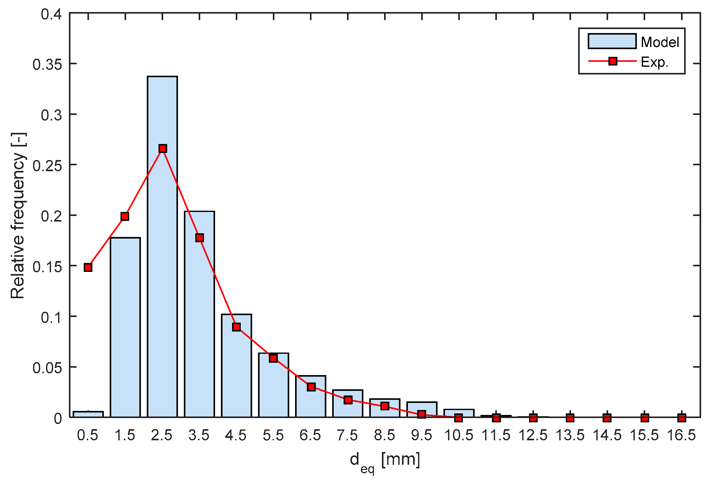
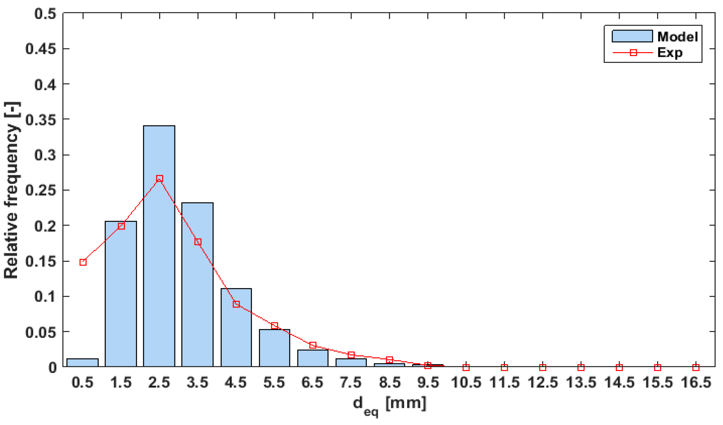
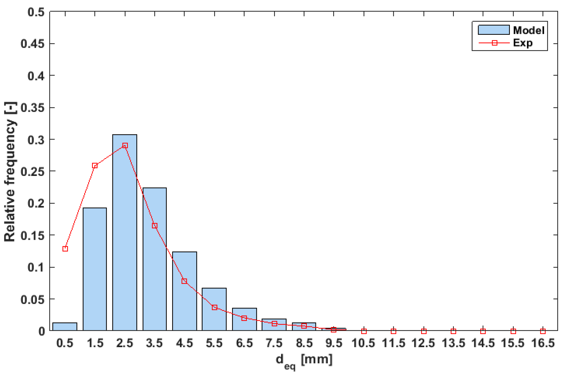
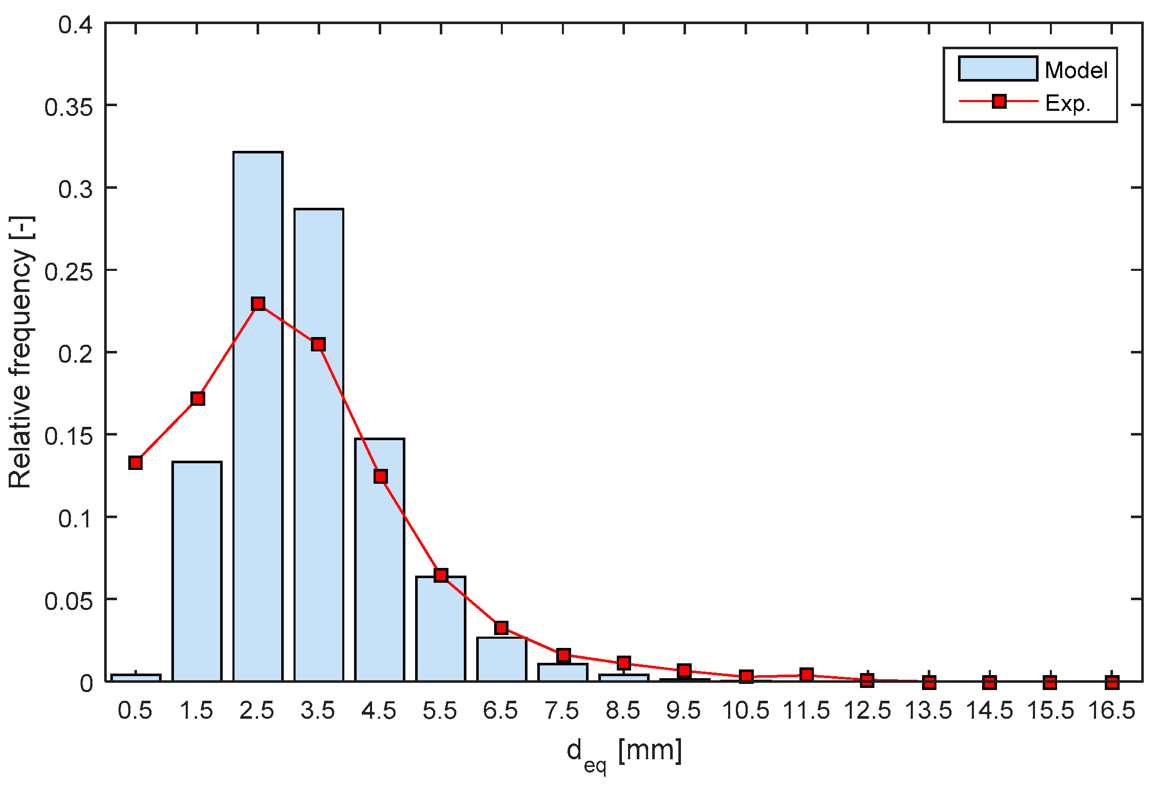
The results of the numerical model are displayed in Figure 2, Figure 3, Figure 4, Figure 5 and Figure 6 for the different gas superficial velocities, UG. In Figure 2, Figure 3, Figure 4, Figure 5 and Figure 6, the labels on the x-axis correspond to the mean value of deq in every class. The predicted BSDs are unimodal with a peak of frequency within the class deq = (2; 3] mm and are, generally, in agreement with the experimental data. It is worth noting that for every UG, the model underestimates the relative frequency of the smallest bubble class (0; 1] mm and overestimates one of the classes (2; 3] mm. At UG = 0.0188 m/s, the shape of the BSD progressively changes (i.e., see the difference between Figure 2 and Figure 6), which is in agreement with the onset of the flow regime transition. In our point of view, the decrease in the Sauter mean diameter from 0.0037 m/s to 0.0111 m/s and its subsequent rise is caused by a change in the prevailing local fluid dynamic phenomena. Possibly, two prevailing mechanisms, determining BSD equilibrium, exist and this behavior is king of a blending between them. Ongoing measurements of BSDs at different axial and radial positions and local liquid velocity profiles aim to clarify this statement. Generally, the BSDs obtained from the model are in good agreement with the experimental BSDs. In addition, the results for the Sauter mean diameter are summarized in Table 1 and show good agreement between the model results and the experimental data. In conclusion, the proposed PBM approach is able to predict bubble size distributions in the bubble column, in the “pseudo-homogeneous” flow regime (which is typical of industrial applications). The model seems to provide reasonable results in terms of bubble size distributions and Sauter mean diameter; therefore, the approach can be applied to estimate the interfacial area for the heat and mass transfer at the interface. In addition, this model may be used to perform sensitivity analyses on operating conditions (i.e., temperature and pressure) for scaling-up purposes. Finally, the proposed approach may be used to predict the flow regime transition, especially if coupled with a lift-force approach. It is worth noting that the mathematical formulation of the model is quite simple and may be easily improved.

4.2. Sensitivity Analyses on Boundary Conditions and Model Closures

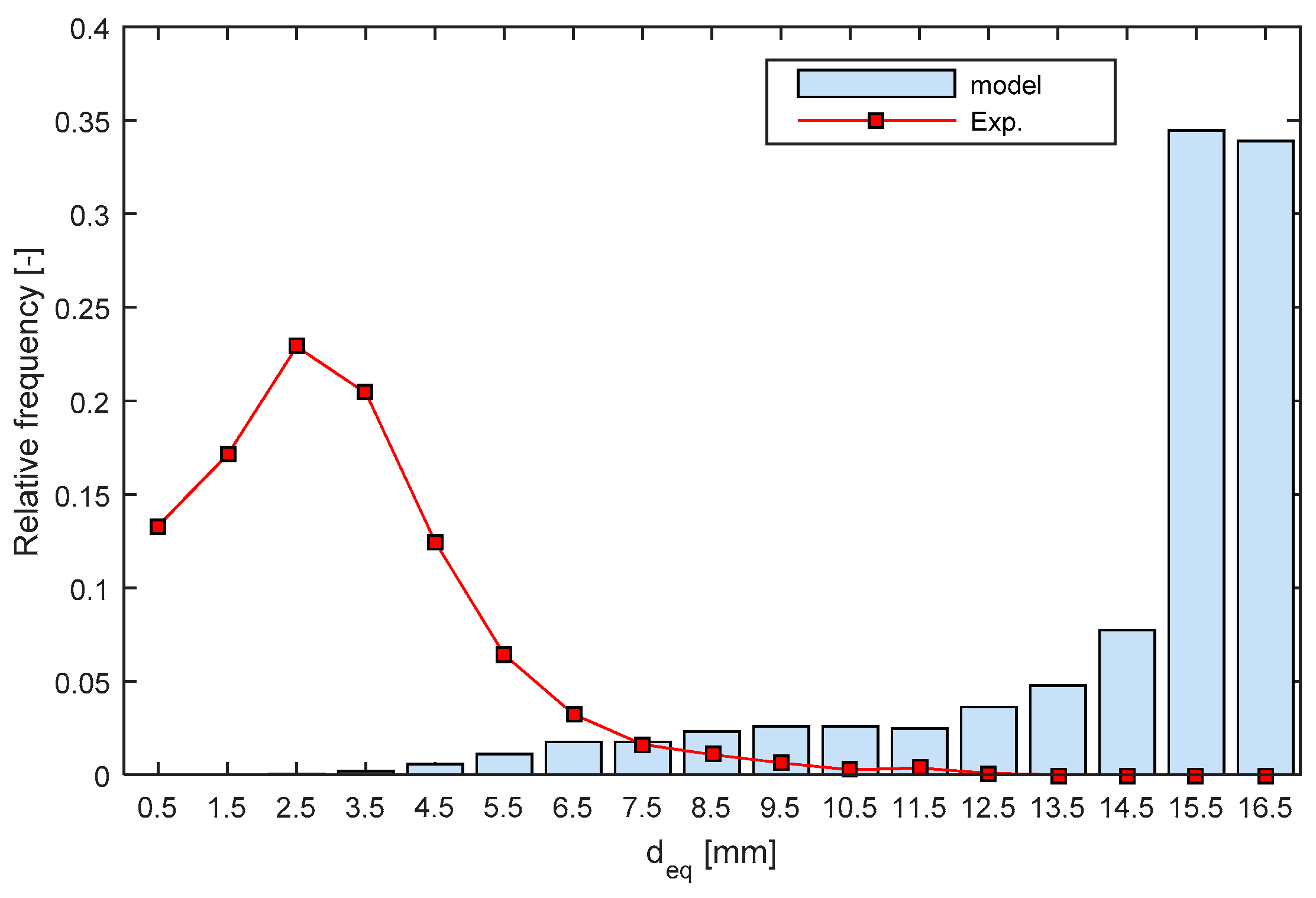
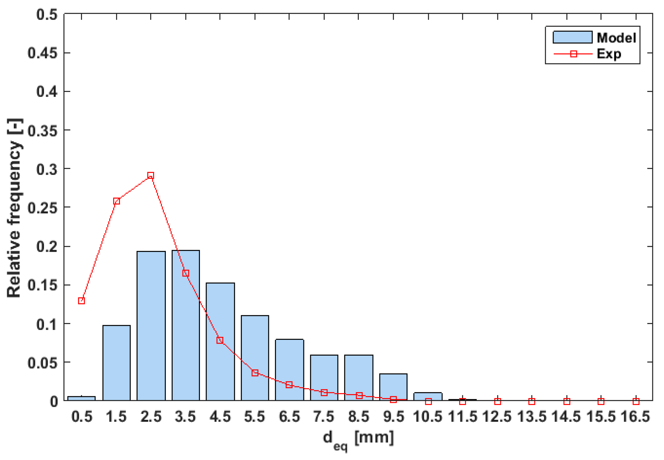
It is interesting to perform sensitivity analyses on the inlet BSD and the constant K (see Equation (33)). When using a uniform BSD as an inlet, the results for the complete range of gas velocities are displayed in Figure 7, Figure 8, Figure 9, Figure 10 and Figure 11. As expected, the model is influenced by the inlet BSD: different initial conditions led to different results. Nevertheless, acceptable results can still be obtained: the proposed model can be used with a uniform inlet BSD as a preliminary tool to support the design of a bubble column. When using the experimental BSD at the sparger along with the original constant proposed by Martinez et al. [23] (K = 0.25), the model is not able to predict the experimental (developed) BSD (Figure 12). The reason is that K determines the breakup frequency and, thus, erroneous modeling determines a different equilibrium point between the coalescence rate and breakup. In Figure 12, for example, the breakup rate is too small to counter-balance the coalescence rate: this issue is the main drawback of the applicability of the present model for performing a scaling-up procedure, as the fitted expression for K is different for different gas distributors and/or different column configurations. Thus, future work should focus on an improved validation of the proposed approach under relevant operating conditions. Possibly, a fitted multi-dimensional map of K-values may be applied in future work. Finally, when using a uniform inlet BSD and the original value of the constant, the model is able to provide first-attempt results, as displayed in Figure 13, Figure 14, Figure 15, Figure 16 and Figure 17. The agreement is lower compared with the modified constant but still acceptable considering the complex gas–liquid flows within the range of gas velocities considered. This result was expected because the model of Martinez et al. [23] was derived for uniform inlet BSD.

5. Conclusions

In this paper, we have contributed to the existing discussion concerning suitable closures for breakup and coalescence in two-phase bubble columns. We have described, formulated, and validated a population balance model to predict the BSDs in the developed region of the bubble column. In particular, we have presented a PBM approach by combining and modifying literature models, and we have validated it against a previously published experimental dataset. The proposed approach is able to correctly estimate BSDs and Sauter mean diameter in the “pseudo-homogeneous” flow regime (which is typical of industrial applications) and can be used, in future studies, to estimate BSDs under relevant operating conditions (high temperature and pressure). It is worth noting that the proposed approach may be improved as follows. Additional coalescence mechanisms may be implemented and the coalescence efficiency formulation may be extended to also consider the mobility of the interfaces. Similarly, the breakup model may be extended to take into account more interactions. In addition, the daughter bubble distribution may be improved to take into account statistical distributions. Finally, these closures may be further extended to predict the BSDs for the other working fluids. Finally, the present model may be coupled with a formulation for the bubble force to predict the local void fraction profiles. In this way, the proposed approach could be extended to predict the whole bubble column fluid dynamics.

Author Contributions

G.B. implemented the PBM approach, conducted the experiments, and wrote the paper; F.I. helped during the experimentation and reviewed the paper.

Funding

This research received no external funding

Conflicts of Interest

The authors declare no conflict of interest

References

  1. Besagni, G.; Inzoli, F. Comprehensive experimental investigation of counter-current bubble column hydrodynamics: Holdup, flow regime transition, bubble size distributions and local flow properties. Chem. Eng. Sci. 2016, 146, 259–290. [Google Scholar] [CrossRef]
  2. Colella, D.; Vinci, D.; Bagatin, R.; Masi, M.; Bakr, E.A. A study on coalescence and breakage mechanisms in three different bubble columns. Chem. Eng. Sci. 1999, 54, 4767–4777. [Google Scholar] [CrossRef]
  3. Lehr, F.; Mewes, D. A transport equation for the interfacial area density applied to bubble columns. Chem. Eng. Sci. 2001, 56, 1159–1166. [Google Scholar] [CrossRef]
  4. Ramkrishna, D.; Mahoney, A.W. Population balance modeling. Promise for the future. Chem. Eng. Sci. 2002, 57, 595–606. [Google Scholar] [CrossRef]
  5. Wilkinson, P.M.; Spek, A.P.; van Dierendonck, L.L. Design Parameters Estimation for Scale-Up of High-Pressure Bubble Columns. AIChE J. 1992, 38, 544–554. [Google Scholar] [CrossRef]
  6. Kataoka, I.; Ishii, M. Drift flux model for large diameter pipe and new correlation for pool void fraction. Int. J. Heat Mass Transf. 1987, 30, 1927–1939. [Google Scholar]
  7. Liao, Y.; Lucas, D. A literature review on mechanisms and models for the coalescence process of fluid particles. Chem. Eng. Sci. 2010, 65, 2851–2864. [Google Scholar] [CrossRef]
  8. Shimizu, K.; Takada, S.; Minekawa, K.; Kawase, Y. Phenomenological model for bubble column reactors: Prediction of gas hold-ups and volumetric mass transfer coefficients. Chem. Eng. J. 2000, 78, 21–28. [Google Scholar] [CrossRef]
  9. Prince, M.J.; Blanch, H.W. Bubble coalescence and break-up in air-sparged bubble columns. AIChE J. 1990, 36, 1485–1499. [Google Scholar] [CrossRef]
  10. Kennard, E.H. Kinetic Theory of Gases, with an Introduction to Statistical Mechanics; McGraw-Hill Book Company, Inc.: New York, NY, USA, 1938. [Google Scholar]
  11. Hughmark, G. Holdup and mass transfer in bubble columns. Ind. Eng. Chem. Process Des. Dev. 1967, 6, 218–220. [Google Scholar] [CrossRef]
  12. Narsimhan, G.; Gupta, J.; Ramkrishna, D. A model for transitional breakage probability of droplets in agitated lean liquid-liquid dispersions. Chem. Eng. Sci. 1979, 34, 257–265. [Google Scholar] [CrossRef]
  13. Shah, Y.; Kelkar, B.G.; Godbole, S.; Deckwer, W.D. Design parameters estimations for bubble column reactors. AIChE J. 1982, 28, 353–379. [Google Scholar] [CrossRef]
  14. Friedlander, S. Smoke, Dust, and Haze: Fundamentals of Aerosol Behavior; J. W. Sons: New York, NY, USA, 1977. [Google Scholar]
  15. Lin, T.J.; Reese, J.; Hong, T.; Fan, L.S. Quantitative analysis and computation of two-dimensional bubble columns. AIChE J. 1996, 42, 301–318. [Google Scholar] [CrossRef]
  16. Coulaloglou, C.; Tavlarides, L. Description of interaction processes in agitated liquid-liquid dispersions. Chem. Eng. Sci. 1977, 32, 1289–1297. [Google Scholar] [CrossRef]
  17. Chesters, A.; Hofman, G. Bubble coalescence in pure liquids. In Mechanics and Physics of Bubbles in Liquids; Springer: Dordrecht, The Netherlands, 1982; pp. 353–361. [Google Scholar]
  18. Kirkpatrick, R.; Lockett, M. The influence of approach velocity on bubble coalescence. Chem. Eng. Sci. 1974, 29, 2363–2373. [Google Scholar] [CrossRef]
  19. Kim, J.W.; Lee, W.K. Coalescence behavior of two bubbles in stagnant liquids. J. Chem. Eng. Jpn. 1987, 20, 448–453. [Google Scholar] [CrossRef]
  20. Levich, V.G.; Technica, S. Physicochemical Hydrodynamics; Prentice-hall: Englewood: Cliffs, NJ, USA, 1962. [Google Scholar]
  21. Azbel, D.; Athanasios, I. A mechanism of liquid entrainment. In Handbook of Fluids in Motion; Ann Arbor Science Publishers: Boston, MA, USA, 1983; p. 473. [Google Scholar]
  22. Lasheras, J.C.; Eastwood, C.; Martınez-Bazán, C.; Montanes, J. A review of statistical models for the break-up of an immiscible fluid immersed into a fully developed turbulent flow. Int. J. Multiph. Flow 2002, 28, 247–278. [Google Scholar] [CrossRef]
  23. Martinez-Bazan, C.; Montanes, J.; Lasheras, J.C. On the breakup of an air bubble injected into a fully developed turbulent flow. Part 1. Breakup frequency. J. Fluid Mech. 1999, 401, 157–182. [Google Scholar] [CrossRef]
  24. Batchelor, G.K. The Theory of Homogeneous Turbulence; Cambridge University Press: Cambridge, UK, 1953. [Google Scholar]
  25. Liao, Y.; Lucas, D. A literature review of theoretical models for drop and bubble breakup in turbulent dispersions. Chem. Eng. Sci. 2009, 64, 3389–3406. [Google Scholar] [CrossRef]
  26. Besagni, G.; Brazzale, P.; Fiocca, A.; Inzoli, F. Estimation of bubble size distributions and shapes in two-phase bubble column using image analysis and optical probes. Flow Meas. Instrum. 2016, 52, 190–207. [Google Scholar] [CrossRef]
Figure 1. The experimental setup.
Computation 07 00017 g001
Figure 2. Comparison between the population balance model (PBM) results and experimental data: UG = 0.0037 m/s.
Computation 07 00017 g002
Figure 3. Comparison between PBM results and experimental data: UG = 0.0074 m/s.
Computation 07 00017 g003
Figure 4. Comparison between PBM results and experimental data: UG = 0.0111 m/s.
Computation 07 00017 g004
Figure 5. Comparison between PBM results and experimental data: UG = 0.0149 m/s.
Computation 07 00017 g005
Figure 6. Comparison between PBM results and experimental data: UG = 0.0188 m/s.
Computation 07 00017 g006
Figure 7. Comparison between PBM and experimental data: uniform bubble size distribution (BSD) at the inlet: UG = 0.0037 m/s.
Computation 07 00017 g007
Figure 8. Comparison between PBM and experimental data: uniform BSD at the inlet: UG = 0.0074 m/s.
Computation 07 00017 g008
Figure 9. Comparison between PBM and experimental data: uniform BSD at the inlet: UG = 0.0111 m/s.
Computation 07 00017 g009
Figure 10. Comparison between PBM and experimental data: uniform BSD at the inlet: UG = 0.0149 m/s.
Computation 07 00017 g010
Figure 11. Comparison between PBM and experimental data: uniform BSD at the inlet: UG = 0.0188 m/s.
Computation 07 00017 g011
Figure 12. Comparison between PBM and experimental data: Martinez constant and real BSD at the inlet: UG = 0.0033 m/s.
Computation 07 00017 g012
Figure 13. Comparison between PBM results and experimental data: Martinez constant and uniform BSD at the inlet: UG = 0.0037 m/s.
Computation 07 00017 g013
Figure 14. Comparison between PBM results and experimental data: Martinez constant and uniform BSD at the inlet: UG = 0.0074 m/s.
Computation 07 00017 g014
Figure 15. Comparison between PBM results and experimental data: Martinez constant and uniform BSD at the inlet: UG = 0.0111 m/s.
Computation 07 00017 g015
Figure 16. Comparison between PBM results and experimental data: Martinez constant and uniform BSD at the inlet: UG = 0.0149 m/s.
Computation 07 00017 g016
Figure 17. Comparison between PBM results and experimental data: Martinez constant and uniform BSD at the inlet: UG = 0.0188 m/s.
Computation 07 00017 g017
Table 1. Comparison between the population balance model (PBM) results and experimental data: Sauter mean diameter, d23.
UG [m/s]0.00370.00740.01110.01490.01880.0037
d23 [mm]—Experimental5.445.514.874.54.875.44
d23 [mm]—Model5.175.875.814.744.565.17