Embedded Exponentially-Fitted Explicit Runge-Kutta-Nyström Methods for Solving Periodic Problems

Abstract

In this work, a pair of embedded explicit exponentially-fitted Runge–Kutta–Nyström methods is formulated for solving special second-order ordinary differential equations (ODEs) with periodic solutions. A variable step-size technique is used for the derivation of the 5(3) embedded pair, which provides a cheap local error estimation. The numerical results obtained signify that the new adapted method is more efficient and accurate compared with the existing methods.

1. Introduction

In this work, we focus on the numerical solution of the special second-order ordinary differential equation of the form:

$$y^{″}=f(x,y),y\left(x_0\right)=y_0,y^{\prime }\left(x_0\right)=y_0^{\prime },$$

(1)

whose solution have a notable periodic character, where $y\in {\Re }^d$ and $f:\Re \times {\Re }^d\to {\Re }^d$ is sufficiently differentiable. Problems of such form occur frequently in the scientific areas such as molecular dynamics, quantum mechanics, chemistry, nuclear physics, and electronics. Due to its applications, many researchers are motivated to study the numerical solution of Equation (1) (see [1,2,3,4,5,6,7]). Senu [8] proposed an embedded explicit RKN method for solving oscillatory problems, Fawzi et al. [9] derived an embedded 6(5) pair of explicit Runge–Kutta methods for periodic ivps, Franco [10] developed two new embedded pairs of explicit Runge–Kutta methods adapted to the numerical solution of oscillatory problems, and Anastassi [11] constructed a 6(4) optimized embedded Runge–Kutta–Nyström pair for the numerical solution of periodic problems. Recently, Demba et al. [12,13] constructed two new embedded explicit trigonometrically-fitted RKN methods for solving the problem in Equation (1). A new embedded explicit exponentially-fitted RKN method based on the 5(3) embedded pair of explicit type derived in [14] is constructed in this work for solving Equation (1). This method can integrate exactly the test equation $y^{{}^{″}}=w^{2}y$, and the numerical results show the efficiency of the proposed method in comparison with other existing RKN methods in the scientific literature.

The paper is structured as follows. In Section 2, we explain the fundamental concepts of an explicit RKN pair, the basic definition of exponentially-fitted RKN method, and the derivation of an explicit exponentially-fitted RKN method. Section 3 deals with the construction of the proposed method. In Section 4, we analyze the algebraic order of the constructed method from their local truncation error (LTE) and we present a detailed information about the stability of the constructed method. In Section 5, we give the numerical results. In Section 6, we present a brief discussion about the graphs obtained, and a conclusion is drawn in the last section of the paper.

2. Fundamental Concepts

A Runge–Kutta–Nyström method of explicit type is represented generally as:

$$\begin{array}{ccc}\hfill y_{n+1}& =& y_n+h{y}_n^{\prime }+h^2\sum _{i=1}^s{b}_{i}f(x_n+c_{i}h,Y_i),\hfill \end{array}$$

(2)

$$\begin{array}{ccc}\hfill y_{n+1}^{\prime }& =& y_n^{\prime }+h\sum _{i=1}^s{d}_{i}f(x_n+c_{i}h,Y_i),\hfill \end{array}$$

(3)

$$\begin{array}{ccc}\hfill Y_i& =& y_n+c_{i}h{y}_n^{\prime }+h^2\sum _{j=1}^{i-1}{a}_{ij}f(x_n+c_{j}h,Y_j).\hfill \end{array}$$

(4)

where $y_{n+1}$ and $y_{n+1}^{\prime }$ denote the approximations of $y\left(x_{n+1}\right)$ and $y^{\prime }\left(x_{n+1}\right)$, respectively, and $x_{n+1}=x_n+h,n=0,1,\dots .$ The corresponding Butcher tableau is given by:

$$\begin{array}{cc}c& A\\ & \\ & b\\ & \\ & d\end{array}$$

where A is a matrix ${\left(a_{ij}\right)}_{s\times s},$ $c={(c_1,c_2,\dots ,c_s)}^T$, $b=(b_1,b_2,\dots ,b_s)$, and $d=(d_1,d_2,\dots ,d_s).$

An embedded $m\left(n\right)$ pair of RKN methods is based on the method $(c,A,b,d)$ of order m and the other RKN method ($c,A,\widehat{b},\widehat{d}$) of order n ($n<m$). The higher order method yields the approximate solution $(y_{n+1}$, $y_{n+1}^{\prime })$, while the lower order method yields the approximate solution $({\widehat{y}}_{n+1},{\widehat{y}}_{n+1}^{\prime })$, which is only used for the estimation of the local truncation error.

A pair of embedded explicit RKN method is generally represented by the following Butcher tableau:

$$\begin{array}{cc}c& A\\ & b^T\\ & d^T\\ & {\widehat{b}}^T\\ & {\widehat{d}}^T\end{array}$$

In this study, a variable step-size procedure is utilized. Local error estimation at the point $x_{n+1}=x_n+h$ is determined by ${\delta }_{n+1}={\widehat{y}}_{n+1}-y_{n+1}$ and ${\delta }_{n+1}^{{}^{\prime }}={\widehat{y}}_{n+1}^{{}^{\prime }}-y_{n+1}^{{}^{\prime }}.$ To control the the step size h, we use the local error estimation given by ${\mathrm{Est}}_{n+1}=\max ({∥{\delta }_{n+1}∥}_{\infty },\parallel {\delta }_{n+1}^{{}^{\prime }}{\parallel }_{\infty })$. We utilize the step-size control procedure in [4] for the numerical solution of Equation (1). That is:

• if $Es{t}_{n+1}<Tol/100,h_{n+1}=2h_n$;
• if $Tol/100\le Es{t}_{n+1}<Tol,h_{n+1}=h_n;$ and
• if $Es{t}_{n+1}\ge Tol,h_{n+1}=h_n/2$ and repeat the step.

Here, $Tol$ is the tolerance. Note that the approximation $y_n$ is used as the initial value for the (n+1)th step.

Definition 1.

A Runge–Kutta–Nyström method (Equations (2)–(4)) is said to be exponentially-fitted if it integrates exactly the functions $e^{wx}$ and $e^{-wx}$ with $w>0$, the principal frequency of the problem.

When an explicit Runge–Kutta–Nyström method (Equations (2)–(4)) is applied to the test equation $y^{{}^{″}}=w^{2}y$, we obtain the following equations:

$$\begin{array}{ccc}\hfill y_{n+1}& =& y_n+hy{{}^{\prime }}_n+h^2\sum _{i=1}^s{b}_i\left(w^2{Y}_i\right),\hfill \end{array}$$

(5)

$$\begin{array}{ccc}\hfill y_{n+1}^{{}^{\prime }}& =& y_n^{\prime }+h\sum _{i=1}^s{d}_i\left(w^2{Y}_i\right),\hfill \end{array}$$

(6)

where

$$\begin{array}{ccc}\hfill Y_1& =& y_n,\hfill \end{array}$$

(7)

$$\begin{array}{ccc}\hfill Y_i& =& y_n+c_{i}h{y}_n^{\prime }+h^2\sum _{j=1}^{i-1}{a}_{ij}\left(w^2{Y}_j\right),i=2,3,\dots ,s.\hfill \end{array}$$

(8)

Let $y_n=e^{w{x}_n}$, evaluating the value of $y_n,y_{n+1}$, $y_n^{\prime }$ and $y_{n+1}^{\prime }$ and, putting in Equations (5)–(8), we get the system of equations below:

$$\begin{array}{ccc}\hfill T_1:={\mathrm{e}}^{\mu }& =& 1+\mu +{\mu }^2\sum _{i=1}^s\left(b_i+b_i{c}_i\mu +b_i{\mu }^2\sum _{j=1}^{i-1}{a}_{\mathit{ij}}{\mathrm{e}}^{-w{x}_n}{Y}_j\right),\hfill \end{array}$$

(9)

$$\begin{array}{ccc}\hfill T_2:={\mathrm{e}}^{\mu }& =& 1+\mu \sum _{i=1}^s\left(d_i+d_i{c}_i\mu +d_i{\mu }^2\sum _{j=1}^{i-1}{a}_{\mathit{ij}}{\mathrm{e}}^{-w{x}_n}{Y}_j\right).\hfill \end{array}$$

(10)

where $\mu =wh.$

3. Construction of the Proposed Method

In this section, we construct a new embedded explicit exponentially-fitted RKN method.

In this study, the RKN5(3) embedded pair is used as given in [14]. The coefficients of the method are given in Table 1.

Table 1. RKN5(3) method in [14].

0
$\frac{1}{5}$	$\frac{1}{50}$
$\frac{2}{3}$	$-\frac{1}{27}$	$\frac{7}{27}$
1	$\frac{3}{10}$	$-\frac{2}{35}$	$\frac{9}{35}$
	$\frac{1}{24}$	$\frac{25}{84}$	$\frac{9}{56}$	0
	$\frac{1}{24}$	$\frac{125}{336}$	$\frac{27}{56}$	$\frac{5}{48}$
	$-\frac{5}{24}$	$\frac{125}{168}$	$-\frac{9}{56}$	$\frac{1}{8}$
	$-\frac{1}{12}$	$\frac{25}{42}$	$\frac{9}{28}$	$\frac{1}{6}$

To obtain the adapted method in the embedding procedure, we consider firstly the coefficients of the lower-order method (order 3) in the RKN5(3) pair. We solve the system of equations in Equations (9) and (10) considering those coefficients but taking two of them as unknowns, specifically the parameters ${\widehat{b}}_3,{\widehat{d}}_3$. We obtain the following solution:

$$\begin{array}{ccc}{\widehat{b}}_3\hfill & =\hfill & \frac{9}{280}\frac{42000{\mathrm{e}}^{\mu }-42000-70{\mu }^7-840{\mu }^5-294{\mu }^6-11500{\mu }^3-3250{\mu }^4-42000\mu -27750{\mu }^2-7{\mu }^8}{{\mu }^2\left(7{\mu }^4+1350+70{\mu }^3+900\mu +300{\mu }^2\right)},\hfill \\ {\widehat{d}}_3\hfill & =\hfill & \frac{3}{70}\frac{31500{\mathrm{e}}^{\mu }-31500-7{\mu }^7-294{\mu }^5-70{\mu }^6-3000{\mu }^3-840{\mu }^4-21375\mu -9000{\mu }^2}{\mu \left(7{\mu }^4+1350+70{\mu }^3+900\mu +300{\mu }^2\right)}.\hfill \end{array}$$

(11)

In Taylor series form, we have:

$$\begin{array}{ccc}{\widehat{b}}_3\hfill & =\hfill & -\frac{9}{56}-\frac{1}{300}{\mu }^3-\frac{23}{9000}{\mu }^4+\frac{41}{42000}{\mu }^5-\frac{157}{3024000}{\mu }^6-\frac{4051}{136080000}{\mu }^7-\frac{23299}{4082400000}{\mu }^8+\frac{1087931}{134719200000}{\mu }^9-\frac{3719141}{1616630400000}{\mu }^{10}\hfill \\ & \hfill & +\frac{59764643}{315242928000000}{\mu }^{11}-\frac{283516309}{66201014880000000}{\mu }^{12}+\frac{2524972693}{66201014880000000}{\mu }^{13}-\frac{213318906023}{9532946142720000000}{\mu }^{14}+\frac{4603543083343}{810300422131200000000}{\mu }^{15}\hfill \\ & \hfill & +\cdots ,\hfill \\ {\widehat{d}}_3\hfill & =\hfill & \frac{9}{28}-\frac{1}{600}{\mu }^3-\frac{7}{4500}{\mu }^4+\frac{31}{54000}{\mu }^5+\frac{29}{1134000}{\mu }^6-\frac{4153}{136080000}{\mu }^7-\frac{8741}{2041200000}{\mu }^8+\frac{22901}{4082400000}{\mu }^9-\frac{530767}{404157600000}{\mu }^{10}\hfill \\ & \hfill & +\frac{91271}{8083152000000}{\mu }^{11}+\frac{74720717}{4728643920000000}{\mu }^{12}+\frac{5158878497}{198603044640000000}{\mu }^{13}-\frac{2900378753}{198603044640000000}{\mu }^{14}+\frac{147077961917}{47664730713600000000}{\mu }^{15}\hfill \\ & \hfill & -\frac{8774361379613}{36463518995904000000000}{\mu }^{16}+\cdots .\hfill \end{array}$$

(12)

As $\mu \to 0$, the coefficients ${\widehat{b}}_3$ and ${\widehat{d}}_3$ of the lower-order adapted method reduce to the coefficients of the original lower-order method in the RKN5(3) approach. In a similar way, solving the above system in Equations (9) and (10) using the coefficients of the higher-order method (order 5) taking as unknowns the coefficients $b_3$ and $d_4$, we obtain the following solution:

$$\begin{array}{ccc}{b}_3\hfill & =\hfill & \frac{225}{28}\frac{168{\mathrm{e}}^{\mu }-168-10{\mu }^3-{\mu }^4-57{\mu }^2-168\mu }{{\mu }^2\left(1350+70{\mu }^3+7{\mu }^4+900\mu +300{\mu }^2\right)},\hfill \\ d_4\hfill & =\hfill & \frac{5}{16}\frac{2400{\mathrm{e}}^{\mu }-2400-6{\mu }^5-275{\mu }^3-60{\mu }^4-950{\mu }^2-2150\mu }{\mu \left(42{\mu }^4+10{\mu }^5+{\mu }^6+375{\mu }^2+750+120{\mu }^3+750\mu \right)}.\hfill \end{array}$$

(13)

In Taylor series form, we have:

$$\begin{array}{ccc}{b}_3\hfill & =\hfill & \frac{9}{56}+\frac{1}{1800}{\mu }^4-\frac{13}{75600}{\mu }^5+\frac{29}{1814400}{\mu }^6+\frac{41}{27216000}{\mu }^7+\frac{1433}{816480000}{\mu }^8-\frac{38177}{26943840000}{\mu }^9+\frac{2843}{7185024000}{\mu }^{10}-\frac{2999609}{63048585600000}{\mu }^{11}\hfill \\ & \hfill & +\frac{12016247}{1471133664000000}{\mu }^{12}-\frac{319437773}{39720608928000000}{\mu }^{13}+\frac{7553067077}{1906589228544000000}{\mu }^{14}-\frac{167041111997}{162060084426240000000}{\mu }^{15}+\cdots ,\hfill \\ d_4\hfill & =\hfill & \frac{5}{48}+\frac{1}{16800}{\mu }^6-\frac{1}{28800}{\mu }^7+\frac{1}{129600}{\mu }^8+\frac{1}{2520000}{\mu }^9-\frac{53}{26400000}{\mu }^{10}+\frac{9403}{5443200000}{\mu }^{11}-\frac{16423}{19656000000}{\mu }^{12}+\frac{2244419}{10478160000000}{\mu }^{13}\hfill \\ & \hfill & +\frac{1078223}{44906400000000}{\mu }^{14}-\frac{211491487}{3113510400000000}{\mu }^{15}+\frac{3036653827}{63154728000000000}{\mu }^{16}+\cdots .\hfill \end{array}$$

(14)

As $\mu \to 0$, the coefficients $b_3$ and $d_4$ of the higher-order adapted method reduce to the coefficients of the original higher-order method in the RKN5(3) approach.

The obtained coefficients depending on $\mu$ together with the rest of coefficients of the original RKN5(3) method form the new adapted embedded method, which is named as EEERKN5(3).

4. Algebraic Order and Error Analysis

In this part, we carry out the local truncation error and orders of convergence analysis based on the Taylor series expansion as given below:

$$\begin{array}{cc}LTE\hfill & =y_{n+1}-y(x_n+h),\hfill \\ LT{E}_{der}\hfill & =y_{n+1}^{{}^{\prime }}-y^{{}^{\prime }}(x_n+h).\hfill \end{array}$$

(15)

The $LTE$ and $LT{E}_{der}$ of the lower-order method (order 3) are:

$$\begin{array}{ccc}LTE\hfill & =\hfill & -\frac{h^4}{24}(f_{xx}+2y^{\prime }{f}_{xy}+{\left(y^{\prime }\right)}^2{f}_{yy}+f_y{y}^{″})+O\left(h^5\right),\hfill \\ LT{E}_{der}\hfill & =\hfill & \frac{h^4}{24}(f_{xxx}+3y^{\prime }{f}_{yxx}+3y^{″}{f}_{xy}+3{\left(y^{\prime }\right)}^2{f}_{xyy}+3y^{\prime }{f}_{yy}{y}^{″}\hfill \\ \hfill & \hfill & +{\left(y^{\prime }\right)}^3{f}_{yyy}+f_y{f}_x+{\left(f_y\right)}^2{y}^{\prime })+O\left(h^5\right).\hfill \end{array}$$

(16)

From Equation (16), we can observe that the algebraic order of the lower-order method is 3 because all of the coefficients up to $h^3$ turns to zero. Similarly, the $LTE$ and $LT{E}_{der}$ of the higher-order method (order 5) are:

$$\begin{array}{ccc}LTE\hfill & =\hfill & \frac{h^6}{21600}(4{y^{\prime }}^3+3{y^{″}}^2{f}_{yy}+6y^{″}{f}_{yxx}+6{y^{\prime }}^2{f}_{xxyy}+{y^{\prime }}^4{f}_{yyyy}+4y^{\prime }{f}_{xxxy}+12f_y{f}_{xx}+12{f_y}^2{y}^{″}\hfill \\ & \hfill & +6{y^{\prime }}^2{f}_{yyy}{y}^{″}+12{y^{\prime }}^2{f}_{yy}{f}_y+12y^{\prime }{f}_{xyy}{y}^{″}+24f_y{y}^{\prime }{f}_{xy}+f_{xxxx}-12w^4{y}^{″})+O\left(h^7\right),\hfill \\ LT{E}_{der}\hfill & =\hfill & \frac{h^6}{720}(f_{xxxxx}+18y^{\prime }{f}_{yy}{f}_y{y}^{″}+15{y^{″}}^2{f}_{xyy}+10y^{″}{f}_{xxxy}+10y^{″}{f}_{xxxy}+10y^{\prime }{f_{xy}}^2+{f_y}^2{f}_x+5f_{xx}{f}_{xy}\hfill \\ & \hfill & +f_y{f}_{xxx}+{y^{\prime }}^4{f}_{xyyyy}+5y^{\prime }{f}_{xxxxy}+10f_{yxx}{f}_x+10{y^{\prime }}^2{f}_{xxxyy}+10{y^{\prime }}^3{f}_{xxyyy}+5{y^{\prime }}^3{f_{yy}}^2+{y^{\prime }}^5{f}_{yyyyy}\hfill \\ & \hfill & +15y^{\prime }{f}_{yyy}{y^{″}}^2+11{y^{\prime }}^3{f}_{yyy}{f}_y+30y^{\prime }{f}_{xxyy}{y}^{″}+30{y^{\prime }}^2{f}_{xyyy}{y}^{″}+8f_y{y}^{″}{f}_{xy}+10y^{″}{f}_{yy}{f}_x+10{y^{\prime }}^3{f}_{yyyy}{y}^{″}\hfill \\ & \hfill & +10{y^{\prime }}^2{f}_{yyy}{f}_x+23{y^{\prime }}^2{f}_y{f}_{xyy}+15{y^{\prime }}^2{f}_{yy}{f}_{xy}+20y^{\prime }{f}_{xyy}{f}_x+13f_y{y}^{\prime }{f}_{yxx}+5y^{\prime }{f}_{yy}{f}_{xx})+O\left(h^7\right).\hfill \end{array}$$

(17)

From Equation (17), the higher-order method has order 5 because all of the coefficients up to $h^5$ turns to zero.

Analysis of Stability

The linear stability of the RKN method in Equations (2)–(4) is obtained by applying it to the test equation $y^{{}^{″}}=-w^{2}y$. In particular, for the method given in Table 1, setting $H=-{\left(wh\right)}^2$, the numerical solution satisfies the following recurrence system:

$$G_{n+1}=E\left(H\right)G_n,$$

where

$$G_{n+1}=\left[\begin{array}{c}{y}_{n+1}\\ h{y}_{n+1}^{{}^{\prime }}\end{array}\right],G_n=\left[\begin{array}{c}{y}_n\\ h{y}_n^{{}^{\prime }}\end{array}\right],E\left(H\right)=\left[\begin{array}{cc}1+H{b}^T{N}^{-1}e& wh(1+H{b}^T{N}^{-1}c)\\ -wh{d}^T{N}^{-1}e& 1+H{d}^T{N}^{-1}c\end{array}\right],N=I-HA,$$

$A={\left[a_{ij}\right]}_{4\times 4}$ is the corresponding matrix of coefficients and I is the identity matrix of fourth order,

$$b={[b_1,b_2,b_3,b_4]}^T,d={[d_1,d_2,d_3,d_4]}^T,e={[1,1,1,1,1,1]}^T,c={[c_1,c_2,c_3]}^T.$$

It is considered that $E\left(H\right)$ has complex conjugate eigenvalues for sufficiently small values of $\mu$ [15]. With this consideration, a periodic numerical solution is obtained. The periodic behavior depends on the eigenvalues of $E\left(H\right)$, which is called the stability matrix and its characteristic equation can be written as:

$${\lambda }^2-tr\left(E\left(H\right)\right)\lambda +det\left(E\left(H\right)\right)=0$$

.

Definition 2.

An interval $(-H_b,0)$ corresponding to the RKN method in Equations (2)–(4) is said to be an interval of absolute stability if, for all $H\in (-H_b,0)$, it holds that $|{\lambda }_{1,2}|<1$, where ${\lambda }_{1,2}$ are the roots of the above characteristic equation.

Definition 3.

An interval $(-H_p,0)$ corresponding to the RKN method in Equations (2)–(4) is said to be periodic if, for every $H\in (-H_p,0)$, $|{\lambda }_{1,2}|=1$, with ${\lambda }_1\ne {\lambda }_2$, where ${\lambda }_{1,2}$ are the roots of the above characteristic equation.

Using Maple package, as well as the definitions in Equations (2) and (3), we find that the higher-order method of our new embedded pair (EEERKN5(3)) has a non-vanishing interval of absolute stability, while the lower-order method of our new embedded pair (EEERKN5(3)) has a non-vanishing interval of periodicity. Therefore, the higher-order method of our new embedded pair (EEERKN5(3)) has $(-9.48,0)$ as the interval of absolute stability, while the lower-order method of our new embedded pair (EEERKN5(3)) has $(-458.42,0)$ as the interval of periodicity.

5. Numerical Experiments

To show the robustness of the constructed method, we consider the following standard embedded RKN methods for the numerical comparison:

• EEERKN5(3): The new embedded pair constructed in this paper;
• RKN5(3): A 5(3) pair of explicit RKN methods given by Van de Vyver in [14];
• ARKN5(3): A 5(3) pair of explicit ARKN methods derived by Franco in [16];
• RKN6(4)6ER-PFAF: A 6(4) optimized embedded RKN pair obtained by Anastassi and Kosti in [11]; and
• FRKN4: A Runge–Kutta–Nyström pair obtained by Van de Vyver in [17],

They are used to integrate the following periodic initial value problems:

Problem 1.

(Almost Periodic Problem) in [18]

$$\begin{array}{ccc}\hfill y_1^{{}^{″}}& =& -y_1+0.001cos\left(x\right),y_1\left(0\right)=1,y_1^{{}^{\prime }}\left(0\right)=0,\hfill \\ \hfill y_2^{{}^{″}}& =& -y_2+0.001sin\left(x\right),y_2\left(0\right)=0,y_2^{{}^{\prime }}\left(0\right)=0.9995,x\in [0,100].\hfill \end{array}$$

The exact solution is

$$y_1\left(x\right)=cos\left(x\right)+0.0005xcos\left(x\right),$$

$$y_2\left(x\right)=sin\left(x\right)-0.0005xsin\left(x\right),$$

We take $w=1.0$ to apply our method and the adapted methods in [11,16,17].

Problem 2.

(Two-Body Problem) in [19]

$$\begin{array}{ccc}\hfill y_1^{{}^{″}}& =& -\frac{y_1}{{\left({y_1}^2+{y_2}^2\right)}^{\frac{3}{2}}},y_1\left(0\right)=1,y_1^{{}^{\prime }}\left(0\right)=0,\hfill \\ \hfill y_2^{{}^{″}}& =& -\frac{y_2}{{\left({y_1}^2+{y_2}^2\right)}^{\frac{3}{2}}},y_2\left(0\right)=0,y_2^{{}^{\prime }}\left(0\right)=1.\hfill \end{array}$$

The exact solution is

$$y_1\left(x\right)=cosx,$$

$$y_2\left(x\right)=sinx,$$

We solve this problem in $[0,100]$ taking $w=1$ for the adapted methods considered.

Problem 3.

(Almost Periodic Problem) Van de Vyver in [17]

$$\begin{array}{ccc}\hfill y_1^{″}& =& -y_1+ϵcos\left(\mathsf{\Psi }x\right),y_1\left(0\right)=1,y_1^{\prime }\left(0\right)=0,\hfill \\ \hfill y_2^{″}& =& -y_2+ϵsin\left(\mathsf{\Psi }x\right),y_2\left(0\right)=0,y_2^{\prime }\left(0\right)=1,x\in [0,100].\hfill \end{array}$$

The exact solution is

$$y_1\left(x\right)=\frac{(1-ϵ-{\mathsf{\Psi }}^2)}{(1-{\mathsf{\Psi }}^2)}cos\left(x\right)+\frac{ϵ}{(1-{\mathsf{\Psi }}^2)}cos\left(\mathsf{\Psi }x\right),$$

$$y_2\left(x\right)=\frac{(1-ϵ\mathsf{\Psi }-{\mathsf{\Psi }}^2)}{(1-{\mathsf{\Psi }}^2)}sin\left(x\right)+\frac{ϵ}{(1-{\mathsf{\Psi }}^2)}sin\left(\mathsf{\Psi }x\right),$$

where $ϵ=0.001$ and $\mathsf{\Psi }=0.1$.

For the application of the adapted method developed in this paper and the methods by Anastassi and Kosti in [11], Franco in [16], and Van de Vvyver in [17], we consider $w=1$.

Problem 4.

(Nonlinear Problem) in [20]

$$y^{″}+y+y^3=Bcos\left(\mathsf{\Omega }x\right),y\left(0\right)=1,y^{\prime }\left(0\right)=0,$$

with $B=0.002$ and $\mathsf{\Omega }=1.01$, the exact solution is

$$y\left(x\right)=0.200179477536cos\left(\mathsf{\Omega }x\right)+0.246946143\times {10}^{-3}cos\left(3\mathsf{\Omega }x\right)+0.304016\times {10}^{-6}cos\left(5\mathsf{\Omega }x\right)+0.374\times {10}^{-9}cos\left(7\mathsf{\Omega }x\right)$$

.

We solve this problem in $[0,100]$ taking $w=1$ for the adapted methods considered.

The numerical results are shown in Table 2, Table 3, Table 4 and Table 5.

Table 2. Numerical results for Problem 1.

TOL	METHOD	STEP	FCN	FSTEP	MAXE	TIME(s)
${10}^{-2}$	EEERKN5(3)	122	488	0	2.570495(−3)	0.053
	RKN5(3)	122	488	0	1.076884(−2)	0.094
	ARKN5(3)	242	968	0	9.829659(−1)	0.271
	RKN6(4)6ER-PFAF	242	1452	0	6.005192(−1)	0.075
	FRKN4	484	1939	1	3.086156(−1)	0.063
${10}^{-4}$	EEERKN5(3)	522	2088	0	4.246848(−7)	0.050
	RKN5(3)	522	2088	0	7.153723(−6)	0.055
	ARKN5(3)	1044	4179	1	6.406274(−2)	0.062
	RKN6(4)6ER-PFAF	1044	6269	1	3.549698(−2)	0.370
	FRKN4	4169	16,685	3	4.185123(−3)	0.102
${10}^{-6}$	EEERKN5(3)	1123	4492	0	4.226820(−9)	0.047
	RKN5(3)	1123	4492	0	1.541216(−7)	0.053
	ARKN5(3)	4491	17,970	2	3.460856(−3)	0.053
	RKN6(4)6ER-PFAF	4491	26,956	2	1.912992(−3)	0.218
	FRKN4	35,919	143,691	5	5.635773(−5)	0.487
${10}^{-8}$	EEERKN5(3)	2420	9680	0	4.243372(−11)	0.075
	RKN5(3)	2420	9680	0	3.319323(−9)	0.096
	ARKN5(3)	19,347	77,397	3	1.863540(−4)	0.130
	RKN6(4)6ER-PFAF	19,347	116,097	3	1.030210(−4)	0.129
	FRKN4	309,539	1,238,177	7	7.583321(−7)	3.248
${10}^{-10}$	EEERKN5(3)	10,422	41,694	2	1.646495(−11)	0.134
	RKN5(3)	10,421	41,687	1	1.664952(−11)	0.109
	ARKN5(3)	83,362	333,460	4	1.003239(−5)	0.338
	RKN6(4)6ER-PFAF	83,362	500,192	4	5.548769(−6)	0.403
	FRKN4	2,667,524	10,670,123	9	1.495822(−8)	26.747

Table 3. Numerical results for Problem 2.

TOL	METHOD	STEP	FCN	FSTEP	MAXE	TIME(s)
${10}^{-2}$	EEERKN5(3)	122	488	0	1.227156(−1)	0.040
	RKN5(3)	122	488	0	8.478978(−1)	0.041
	ARKN5(3)	270	1083	1	1.804551(+0)	0.044
	RKN6(4)6ER-PFAF	363	2188	2	1.815228(+0)	0.047
	FRKN4	484	1939	1	1.942861(+0)	0.043
${10}^{-4}$	EEERKN5(3)	522	2088	0	3.621045(−5)	0.041
	RKN5(3)	522	2088	0	6.990118(−4)	0.047
	ARKN5(3)	1044	4179	1	1.480069(−1)	0.045
	RKN6(4)6ER-PFAF	1044	6269	1	2.961366(−1)	0.041
	FRKN4	4169	16,685	3	1.130567(−2)	0.078
${10}^{-6}$	EEERKN5(3)	1123	4492	0	3.722093(−7)	0.054
	RKN5(3)	1123	4492	0	1.520229(−5)	0.063
	ARKN5(3)	4491	17,970	2	5.473843(−3)	0.051
	RKN6(4)6ER-PFAF	4491	26,956	2	6.609722(−3)	0.060
	FRKN4	35,919	143,691	5	1.165965(−4)	0.361
${10}^{-8}$	EEERKN5(3)	2420	9680	0	3.718493(−9)	0.058
	RKN5(3)	2420	9680	0	3.282692(−7)	0.139
	ARKN5(3)	19,347	77,397	3	4.588825(−4)	0.122
	RKN6(4)6ER-PFAF	19,347	116,097	3	2.397332(−4)	0.090
	FRKN4	309,539	1,238,177	7	1.515111(−6)	2.676
${10}^{-10}$	EEERKN5(3)	10,422	41,694	2	1.717850(−11)	0.120
	RKN5(3)	10,421	41,687	1	2.058225(−10)	0.054
	ARKN5(3)	83,362	333,460	4	2.680717(−5)	0.254
	RKN6(4)6ER-PFAF	83,362	500,192	4	1.145927(−5)	0.247
	FRKN4	2,667,524	10,670,123	9	1.557560(−8)	22.647

Table 4. Numerical results for Problem 3.

TOL	METHOD	STEP	FCN	FSTEP	MAXE	TIME(s)
${10}^{-2}$	EEERKN5(3)	122	488	0	2.591319(−3)	0.062
	RKN5(3)	122	488	0	1.078825(−2)	0.062
	ARKN5(3)	242	968	0	9.806283(−1)	0.100
	RKN6(4)6ER-PFAF	242	1452	0	5.976002(−1)	0.300
	FRKN4	484	1939	1	3.076264(−1)	0.092
${10}^{-4}$	EEERKN5(3)	522	2088	0	4.299671(−7)	0.065
	RKN5(3)	522	2088	0	7.172465(−6)	0.074
	ARKN5(3)	1044	4179	1	6.403390(−2)	0.191
	RKN6(4)6ER-PFAF	1044	6269	1	3.548404(−2)	0.165
	FRKN4	4169	16,685	3	4.181655(−3)	0.126
${10}^{-6}$	EEERKN5(3)	1123	4492	0	4.355510(−9)	0.064
	RKN5(3)	1123	4491	0	1.542823(−7)	0.066
	ARKN5(3)	4491	17,970	2	3.458063(−3)	0.152
	RKN6(4)6ER-PFAF	4491	26,956	2	1.911456(−3)	0.143
	FRKN4	35,919	143,691	5	5.631169(−5)	0.566
${10}^{-8}$	EEERKN5(3)	2420	9680	0	4.516099(−11)	0.081
	RKN5(3)	2420	9680	0	3.324929(−9)	0.095
	ARKN5(3)	19,347	77,397	3	1.862032(−4)	0.243
	RKN6(4)6ER-PFAF	19,347	116,097	3	1.029369(−4)	0.276
	FRKN4	309,539	1,238,177	7	7.577131(−7)	3.588
${10}^{-10}$	EEERKN5(3)	10,422	41,694	2	1.643935(−11)	0.166
	RKN5(3)	10,421	41,687	1	1.658362(−11)	0.153
	ARKN5(3)	83,362	333,460	4	1.002430(−5)	0.470
	RKN6(4)6ER-PFAF	83,362	500,192	4	5.544237(−6)	0.470
	FRKN4	2,667,524	10,670,123	9	1.494338(−8)	26.650

Table 5. Numerical results for Problem 4.

TOL	METHOD	STEP	FCN	FSTEP	MAXE	TIME(s)
${10}^{-2}$	EEERKN5(3)	122	515	9	1.170545(−3)	0.055
	RKN5(3)	122	536	16	2.777502(−3)	0.066
	ARKN5(3)	123	504	4	2.849535(−1)	0.141
	RKN6(4)6ER-PFAF	124	744	0	2.653779(−1)	0.062
	FRKN4	439	1825	23	5.355312(−2)	0.062
${10}^{-4}$	EEERKN5(3)	262	1072	8	1.356514(−5)	0.047
	RKN5(3)	262	1075	9	7.208088(−5)	0.062
	ARKN5(3)	510	2076	12	4.321049(−2)	0.078
	RKN6(4)6ER-PFAF	513	3128	10	2.781421(−2)	0.094
	FRKN4	1815	7362	34	2.600772(−3)	0.088
${10}^{-6}$	EEERKN5(3)	573	2337	15	9.010356(−8)	0.062
	RKN5(3)	562	2260	4	1.659456(−6)	0.078
	ARKN5(3)	2085	8439	33	1.815951(−3)	0.141
	RKN6(4)6ER-PFAF	2140	13,005	33	1.236425(−3)	0.071
	FRKN4	14,666	58,868	68	4.713910(−5)	0.266
${10}^{-8}$	EEERKN5(3)	1959	7932	32	9.751267(−10)	0.078
	RKN5(3)	2324	9392	32	7.596427(−9)	0.141
	ARKN5(3)	9091	36,487	41	1.005629(−4)	0.148
	RKN6(4)6ER-PFAF	9258	55,773	45	6.549156(−5)	0.187
	FRKN4	134,843	539,678	102	4.210467(−7)	2.129
${10}^{-10}$	EEERKN5(3)	5213	21,140	96	4.741679(−12)	0.109
	RKN5(3)	5183	20,816	28	4.524522(−11)	0.125
	ARKN5(3)	39,556	158,425	67	5.609382(−6)	0.281
	RKN6(4)6ER-PFAF	40,226	241,631	55	3.583863(−6)	0.299
	FRKN4	1,209,331	4,837,732	136	5.483721(−9)	14.829

To further show the efficacy of the constructed method (EEERKN5(3)), we use the graphical approach to display the performance of EEERKN5(3) in comparison with other existing methods in the literature, as shown in Figure 1, Figure 2, Figure 3 and Figure 4. Tol = ${10}^{-2i},i=1,2,3,4,5.$

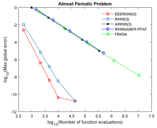
Figure 1. Efficiency curves for Problem 1.

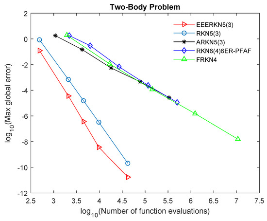
Figure 2. Efficiency curves for Problem 2.

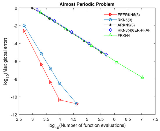
Figure 3. Efficiency curves for Problem 3.

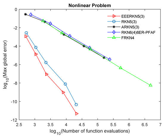
Figure 4. Efficiency curves for Problem 4.

6. Discussion

Our proposed method (EEERKN5(3)) has the least error norm and least computational time, signifying that it is highly efficient and accurate for solving Equation (1), as shown in Table 2, Table 3, Table 4 and Table 5 and Figure 1, Figure 2, Figure 3 and Figure 4. The graphs show the accuracy, measured in ${log}_{10}\left(Maxglobalerror\right)$ versus the ${log}_{10}\left(Numberoffunctionevaluations\right)$. Therefore, we can deduce that (EEERKN5(3)) is more suitable for solving Equation (1) than the other existing methods in the scientific literature.

7. Conclusions

In this work, we construct a new efficient embedded explicit exponentially-fitted RKN method for solving periodic initial value problems. The constructed method contains four variable coefficients that depend on a parameter which is given by the product of the parameter of the method w and the step-length h [21,22]. The numerical experiment performed show clearly that EEERKN5(3) is more efficient for solving problem in Equation (1) than the other existing methods used for comparison.

References

- Simos, T.E. Exponentially fitted modified Runge-Kutta-Nyström method for the numerical solution of initial-value problems with oscillating solutions. Appl. Math. Lett. 2002, 15, 217–225. [Google Scholar] [CrossRef]
- Van de Vyver, H. An embedded exponentially-fitted Runge-Kutta-Nyström method for the numerical solution of orbital problems. New Astron. 2006, 11, 577–587. [Google Scholar] [CrossRef]
- Kalogiratou, Z.; Simos, T.E. Construction of trigonometrically-fitted and exponentially-fitted Runge-Kutta-Nyström methods for the numerical solution of schrödinger equation and related problems-a method of 8th algebraic order. J. Math. Chem. 2002, 31, 211–232. [Google Scholar] [CrossRef]
- Liu, S.; Zheng, J.; Fang, Y. A new modified embedded 5(4) pair of explicit Runge-Kutta methods for the numerical solution of schrödinger equation. J. Math. Chem. 2002, 15, 217–225. [Google Scholar] [CrossRef]
- Kosti, A.A.; Anastassi, Z.A. Explicit almost P-stable Runge–Kutta–Nyström methods for the numerical solution of the two-body problem. Comput. Appl. Math. 2015, 34, 647–659. [Google Scholar] [CrossRef]
- Kosti, A.A.; Anastassi, Z.A.; Simos, T.E. Construction of an optimized explicit Runge–Kutta–Nyström method for the numerical solution of oscillatory initial value problems. Comput. Math. Appl. 2011, 61, 3381–3390. [Google Scholar] [CrossRef]
- Ahmad, N.A.; Senu, N. New 4 (3) pair two derivative Runge-Kutta method with FSAL property for solving first order initial value problems. AIP Conf. Proc. 2017, 1870, 040053. [Google Scholar]
- Senu, N.; Suleiman, M.; Ismail, F. An embedded explicit Runge-Kutta-Nyström method for solving oscillatory problems. Phys. Scr. 2009, 80, 015005. [Google Scholar] [CrossRef]
- Fawzi, F.A.; Senu, N.; Ismail, F.; Majid, Z.A. An embedded 6(5) pair of explicit Runge-Kutta method for periodic ivps. Far East J. Math. Sci. 2016, 100, 1841. [Google Scholar] [CrossRef]
- Franco, J.; Khiar, Y.; Randez, L. Two new embedded pairs of explicit Runge-Kutta methods adapted to the numerical solution of oscillatory problems. Appl. Math. Comput. 2014, 232, 416–423. [Google Scholar] [CrossRef]
- Anastassi, Z.; Kosti, A. A 6(4) optimized embedded Runge-Kutta Nyström pair for the numerical solution of periodic problems. J. Comput. Appl. Math. 2015, 275, 311–320. [Google Scholar] [CrossRef]
- Demba, M.A.; Senu, N.; Ismail, F. A 5(4) Embedded Pair of Explicit Trigonometrically-Fitted Runge–Kutta–Nyström Methods for the Numerical Solution of Oscillatory Initial Value Problems. Math. Comput. Appl. 2016, 21, 46. [Google Scholar] [CrossRef]
- Demba, M.A.; Senu, N.; Ismail, F. An Embedded 4(3) Pair of Explicit Trigonometrically-Fitted Runge-Kutta-Nyström Method for Solving Periodic Initial Value Problems. Appl. Math. Sci. 2017, 11, 819–838. [Google Scholar] [CrossRef][Green Version]
- Vyver, H.V. A 5(3) pair of explicit Runge-Kutta-Nyström methods for oscillatory problems. Math. Comput. Model. 2007, 45, 708–716. [Google Scholar] [CrossRef]
- Van der Houwen, P.; Sommeijer, B. Diagonaly implicit Runge-Kutta Nyström methods for oscillatory problems. SIAM J. Numer. Anal. 1989, 26, 414–429. [Google Scholar] [CrossRef]
- Franco, J. A 5(3) pair of explicit ARKN methods for the numerical integration of pertubed oscillators. J. Comput. Appl. Math. 2003, 161, 283–293. [Google Scholar] [CrossRef]
- Vyver, H.V. A Runge-Kutta-Nyström pair for the numerical integration of pertubed oscillators. Comput. Phys. Commun. 2005, 167, 129–142. [Google Scholar] [CrossRef]
- Demba, M.A. Trigonometrically-Fitted Explicit Runge-Kutta-Nyström Methods for Solving Special Second Order Order Differential Equations with Periodic Solutions. Master’s Thesis, Department of Mathematics, Faculty of Science, Serdang, Malaysia, 2016. [Google Scholar]
- Senu, N. Runge-Kutta Nyström Methods for Solving Oscillatory Problems. Ph.D. Thesis, Department of Mathematics, Faculty of Science, Serdang, Malaysia, 2009. [Google Scholar]
- Berghe, G.V.; de Meyer, H.; Marnix, V.D.; Tanja, V.H. Exponentially-fitted explicit Runge–Kutta methods. Comput. Phys. Commun. 1999, 123, 7–15. [Google Scholar] [CrossRef]
- Ramos, H.; Vigo-Aguiar, J. On the frequency choice in trigonometrically fitted methods. Appl. Math. Lett. 2010, 23, 1378–1381. [Google Scholar] [CrossRef]
- Vigo-Aguiar, J.; Ramos, H. On the choice of the frequency in trigonometrically-fitted methods for periodic problems. J. Comput. Appl. Math. 2015, 277, 94–105. [Google Scholar] [CrossRef]
© 2020 by the authors. Licensee MDPI, Basel, Switzerland. This article is an open access article distributed under the terms and conditions of the Creative Commons Attribution (CC BY) license (http://creativecommons.org/licenses/by/4.0/).