Abstract
A class of bivariate integer-valued time series models was constructed via copula theory. Each series follows a Markov chain with the serial dependence captured using copula-based transition probabilities from the Poisson and the zero-inflated Poisson (ZIP) margins. The copula theory was also used again to capture the dependence between the two series using either the bivariate Gaussian or “t-copula” functions. Such a method provides a flexible dependence structure that allows for positive and negative correlation, as well. In addition, the use of a copula permits applying different margins with a complicated structure such as the ZIP distribution. Likelihood-based inference was used to estimate the models’ parameters with the bivariate integrals of the Gaussian or t-copula functions being evaluated using standard randomized Monte Carlo methods. To evaluate the proposed class of models, a comprehensive simulated study was conducted. Then, two sets of real-life examples were analyzed assuming the Poisson and the ZIP marginals, respectively. The results showed the superiority of the proposed class of models.
1. Introduction
Following a similar framework of building bivariate models for ordinal panel data via [1], we constructed a class of bivariate integer-valued time series models using copula theory. Applying either the bivariate Gaussian copula or the bivariate t-copula functions, we jointly modeled two copula-based Markov time series models (see [2,3]). Such a method allows for flexible dependence structures between the two time series and within each one, which allow for both positive or negative correlations, which is theoretically not presented with most existing methods.
The count time series data have multiple applications, many of which have been covered in the literature; see [4] for a comprehensive review. Sometimes, in finance, climate, public health, and crime data analysis, time series counts come as bivariate vectors that observe not only serial dependence within each time series, but also interdependence or cross-dependence between the two series. To accurately study such data, one needs to account for the two types of dependence that emerge from the observed data by applying multivariate time series models. The literature covering normally distributed multivariate time series is plentiful. However, with count time series data and due to the complexity of the computational burden of analyzing such data, the literature on bivariate or multivariate count time series is limited, and so is the zero-inflated cases of time series.
Following the concepts of the integer-valued autoregressive moving average (INARMA) model, Reference [5] introduced the bivariate integer-valued moving average (BINMA) model, which allows for both positive and negative correlation between counts. Further, they presented an extension to the multivariate version starting from the BINMA model. Reference [6] proposed a bivariate zero-inflated Poisson model to analyze occupational injuries. Reference [7] introduced a multivariate autoregressive conditional double Poisson model, which can accommodate overdispersion, serial dependence, and cross-correlation. They used a multivariate normal copula to capture the cross-correlation between time series, and parameter estimation was conducted using a two-stage estimation procedure. The work of [8] presented a bivariate integer-valued autoregressive process (BINAR(1)) in which the cross-correlation was modeled using a copula to accommodate both positive and negative correlation. They presented the use of a Frank and Gaussian copula to model dependence, and marginal time series were modeled using Poisson and negative binomial INAR(1) models. Reference [9] applied state space models for multivariate count time series and used the to analyze marketing datasets. Reference [10] proposed a new bivariate Poisson INGARCH model, which allows for positive or negative cross-correlation between time series. Reference [11] proposed a class of flexible bivariate Poisson INGARCH(1,1) models whose dependence was established by a special multiplicative factor. The parameter estimation was conducted using maximization by parts the algorithm and its modified version to reduce the computation time. Reference [12] proposed a model for longitudinal data where the univariate margins were selected from the class of zero-inflated distributions, and the dependence structure was modeled using a D-vine copula. Reference [13] presented a comprehensive review on a copula and its applications in different fields. They presented the use of a copula in time series under both univariate and multivariate setups. Reference [14] also wrote a comprehensive review, but on multivariate time series for count time series.
The rest of the paper is organized as follows. In Section 2, we first provide a brief background on the Poisson and ZIP regression model and the copula theory. Then, Section 3 presents the proposed class of copula-based bivariate models to analyze two dependent time series, each being modeled via copula-based Markov chains and then jointly handled using either the bivariate Gaussian or t-copula functions. In Section 5, we give some simulation results. Section 6 provides two real data examples. The conclusion is given in Section 7.
2. Background
2.1. The Poisson and ZIP Distributions
The probability mass function (pmf) of the well-known Poisson distribution is defined as:
where is the intensity (mean) parameter. To account for a large number of zeros (zero-inflation), a modified version of the Poisson distribution is given by the zero-inflated Poisson (ZIP), which handles the presence of excess zeros. It is described by two parameters denoted as the extra probability thrust and the intensity parameter This is defined by:
where is the indicator function, is the zero-inflation parameter, and is the intensity parameter, or the mean, of the baseline Poisson distribution. Note that the pmf (1) is a mixture of the degenerate distribution with a point mass at zero and a Poisson distribution. There is a large literature associated with the ZIP, starting from [15] to [16].
2.2. Copula
As a multivariate cumulative distribution function (cdf), the copula is a joint function that captures the dependence structure between variables. With uniform margins as in [17], a p-dimensional copula is a function with the following properties:
- ;
- ;
- For any with for
The copula is unique if the marginal distributions are continuous, but not when some of the components are discrete. In fact, under Sklar’s theorem, if are random variables with marginal distribution functions and joint cumulative distribution function F, then the following hold:
- There exists a p-dimensional copula C such that for all :
- If are continuous, then the copula C is unique. Otherwise, C can be uniquely determined on p- dimensional rectangle
There are a number of copula functions, i.e., C, from which one can choose. Table 1 shows some of the popular functions of the copula families. For more details on these families, see [18].

Table 1.
Bivariate copula functions.
3. Constructing the Bivariate Models
Assume we observe the following series of a two- vector, , where for . Using copula theory, we can separately study and and their joint behavior, which would describe the cross-dependence among the bivariate series and with the assumption that each series and follows a copula-based Markov process (see [2,3,19] for examples).
We were interested in studying the mean vector of the bivariate series, i.e., , and more importantly, the correlation matrix, say , where:
and:
where the diagonal elements of the matrix in (2) describe the autocovariance among each of the two series, while the off-diagonal elements describe the cross-correlation between and .
Hence, observing both types of correlations, the joint probability distribution of and given and , respectively, for , is given by:
where is either the inverse cdf of the normal distribution or the t-distribution with being the bivariate normal or t-distribution, respectively. Here, R is the correlation matrix associated with the bivariate distribution capturing the cross-sectional dependence, given by:
where is a dependence parameter of either the Gaussian or the t-copula function that explains the cross-dependence between the two series. Furthermore, and , for , where:
is the transition cdf of given , for , and:
where is a bivariate copula function with dependence parameter , describing the serial dependence in a single series, and is a vector of the marginal parameters of the ZIP distribution and reduces to a scalar with the Poisson distribution, i.e., .
4. Estimation Method
To draw a likelihood-based inference, the log-likelihood function is built. Such a function has no closed form, so its maximization is presented next.
With the likelihood function construction for , the joint (bivariate) distribution of and is given by:
and for , the conditional bivariate distribution of and given and is given by:
Hence, combining the functions in (4) and (5), the likelihood function is given by:
where , where is the marginal parameter vector and and are the copula parameters to deal with the first and second time series, respectively. The bivariate dependence parameter is captured by . Therefore, taking the log of the function in (6), we obtain the log-likelihood function as follows:
Maximizing the log-likelihood function in (7) provides ML estimates for the proposed class of models. However, within the log-likelihood function exists a bivariate normal or t-integral function that does not have a closed function as shown in (3). Hence, we evaluated the bivariate integral function using the standard randomized importance sampling method introduced by [20], which has been proven to be effective with dimensions less than ten. Then, the parameter estimates, i.e., , can be obtained by:
This maximizing technique produces a numerically calculated Hessian matrix that provides the Fisher information matrix (FIM). Taking the inverse of the FIM yields the standard errors of the ML estimates of . In the next section, we evaluate the proposed class of bivariate models via comprehensive simulation studies to show the effectiveness of the estimation method.
5. Simulation Studies
A comprehensive simulation study was conducted to evaluate the proposed method, and the asymptotic properties of the parameter estimates were validated. For each univariate time series, we considered a copula-based Markov model, where a copula family was used for the joint distribution of subsequent observations, and then, coupled these two time series using another copula at each time point. Here, , denote the means of the marginal distributions. and measure the serial dependence within each time series, and denotes the cross-correlation between two time series. The Gaussian copula and Student’s t-copula were selected as candidate copula families with true parameters ( = 3, = 5, = , = , = ). The simulation was performed using sample sizes of 100, 300, and 500 while replicating it 300 and 500 times. For each of these five parameter estimates, the standard error was calculated, and the results are displayed in Table 2 and Table 3.
Table 2.
Parameter estimates using the Gaussian copula for a univariate and joint distribution for 300 and 500 replicates.
Table 3.
Parameter estimates using the Gaussian copula for univariate distributions and the t-copula for the joint distribution for 300 and 500 replicates.
Table 2 and Table 3 illustrate that the parameter estimates converge to true values as the number of replicates increases and the standard error decreases as the sample size increases. The results showed that the estimates become more and more robust as the sample size increases.
Expanding the results, we performed the simulations for the ZIP choosing the Gaussian copula for the univariate and joint distributions with true parameters ( = 3, = 5, = , = , = , = , = ) where the marginals follow the Poisson or ZIP marginals. here for the zero-inflated Poisson distribution where and represent the zero-inflation parameters for the ZI marginal densities. The results in Table 4 indicate the robustness of the parameter estimates even under negative cross-correlation.
Table 4.
Parameter estimates using the Gaussian copula for the univariate and joint distributions for 300 replicates with the Poisson and ZIP marginals.
6. Applications
The proposed models were applied to two real-life examples, and the results are presented in Section 6.1 and Section 6.2.
6.1. Application to Forgery and Fraud Data
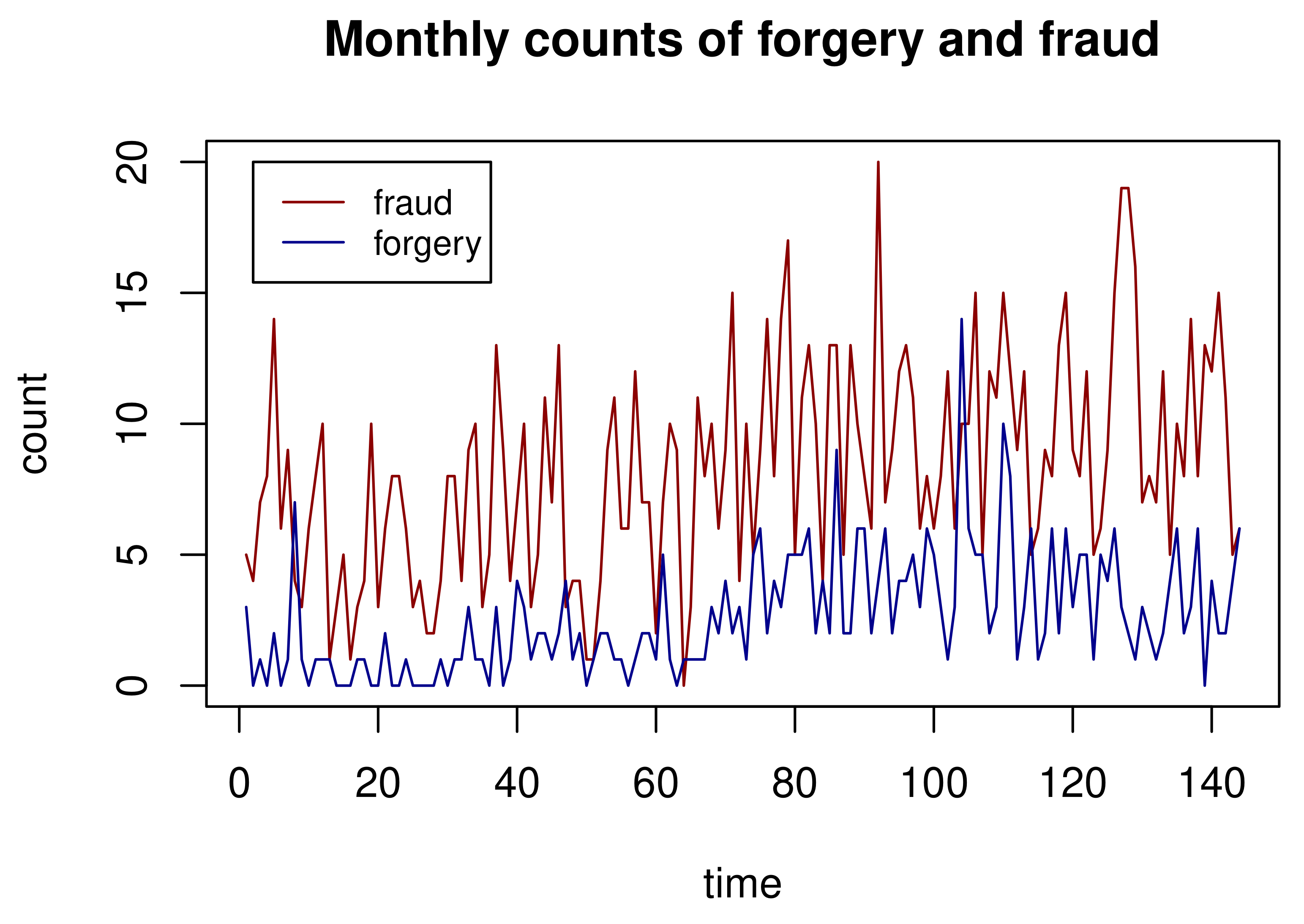
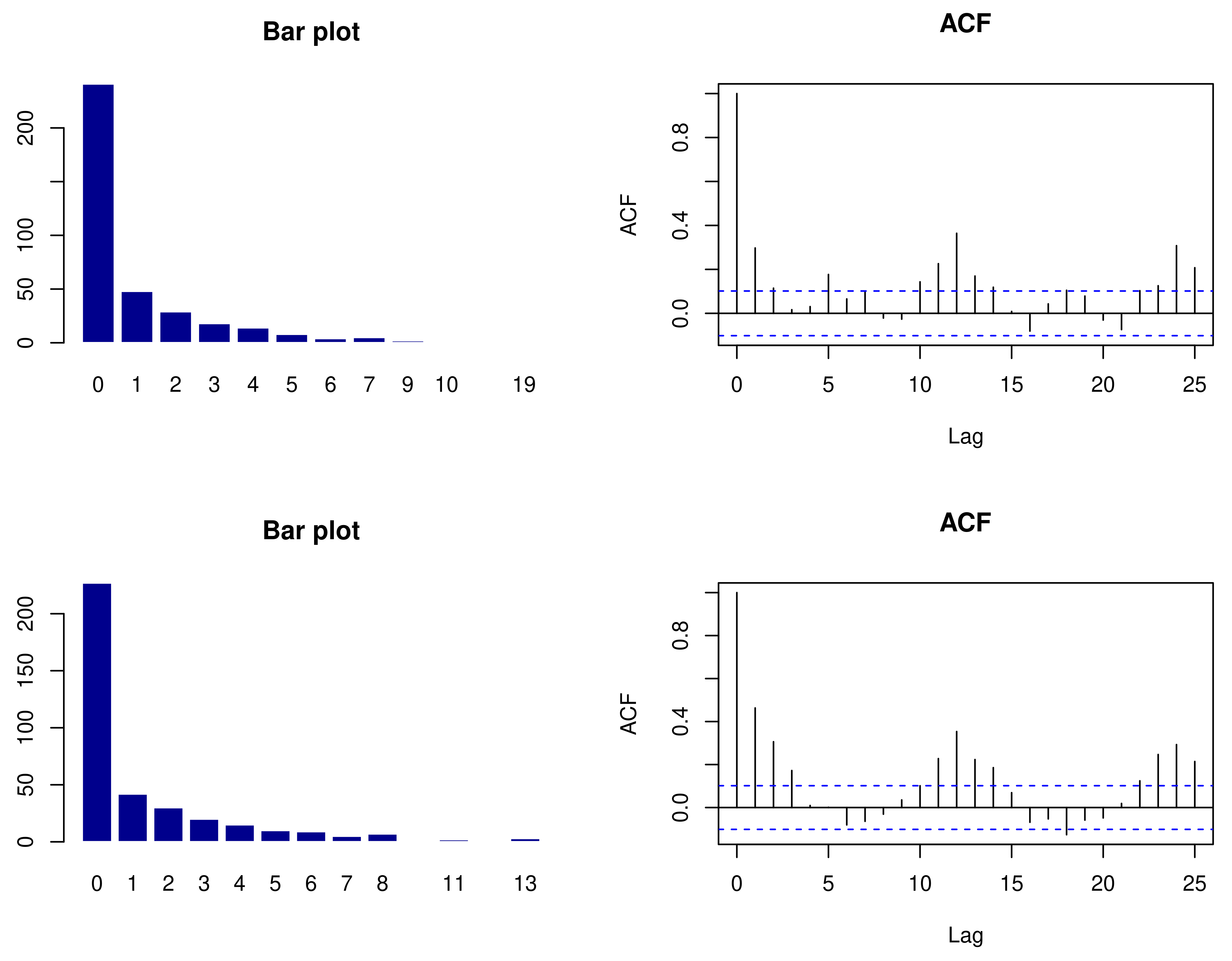
We considered monthly counts of forgery and fraud in the 61st police car beat in Pittsburgh, PA. For a selected county, two count time series were selected to fit the proposed bivariate Poisson class of models. The empirical means for the two count time series were 2.632 and 8.243, respectively. The cross-correlation between the two time series was 0.307, which provided sufficient evidence that the two series are dependent. Monthly counts of forgery and fraud are displayed in Figure 1. The fraud count series has higher counts and larger fluctuations when compared to the fraud time series over time. Figure 2 shows the distributions of the count via bar plots and sample autocorrelation functions (ACFs) for the forgery and Fraud count series, respectively. The bar plots suggest that both counts follow Poisson distributions, whereas the ACFs indicate that the two series are serially dependent. Hence, we can now investigate both types of dependences properly using the proposed method of bivariate Poisson time series.
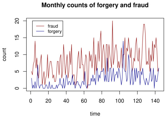
Figure 1.
Forgery and fraud count series.
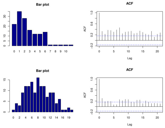
Figure 2.
Bar plot and ACFs for counts of forgery (top) and fraud (bottom).
Different copula families were fit for the univariate and joint distributions, and their corresponding AIC values are reported in Table 5. Parameter estimates and the corresponding standard deviations are recorded in Table 6.
Table 5.
AIC values for the bivariate Poisson model with different copula families.
Table 6.
Parameter estimates for the bivariate Poisson model.
6.2. Application to Sandstorm Data
The dataset used for this application consisted of the monthly count of strong sandstorms recorded by the AQI airport station in Eastern Province, Saudi Arabia. The zero-inflated proportions for the two time series were and , respectively. The cross-correlation between the two time series was 0.465, and this provided evidence that the two counts are cross-correlated. For the proposed BZIP model, the parameter estimates and the corresponding standard deviations are recorded in Table 8.
The two sandstorm count series are shown in Figure 3. The plot shows that there exist the frequent occurrence of zeros for both time series. The bar plots and ACFs of sandstorm counts for Rafha and Qaisumah are shown in Figure 4. The plots show that there exists the frequent occurrence of zeros and low-ordered autocorrelation. Hence, we applied the bivariate ZIP distribution to model the sandstorm counts.
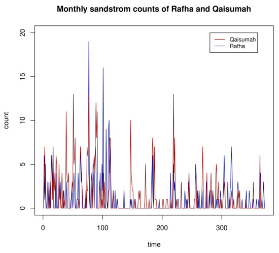
Figure 3.
Sandstorm counts of Rafha and Qaisumah.
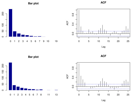
Figure 4.
Bar plot and ACFs for sandstorm counts of Rafha (top) and Qaisumah (bottom).
Different copula families were fit for the univariate and joint distributions, and their corresponding AIC values are reported in Table 7. Table 8 represents the parameter estimates and corresponding standard deviations for the fitted bivariate zero-inflated model using the Gaussian copula for the joint and marginal distributions.
Table 7.
AIC values for the BZIP model with different copula families.
Table 8.
Parameter estimates for the bivariate zero-inflated Poisson model.
The standard errors are very small under both the Poisson and ZIP marginals, which emphasizes the robustness of our proposed method.
7. Summary
In this paper, we proposed a class of bivariate integer-valued time series models that was constructed via copula theory. The use of Markov chains to capture the serial dependence via copula-based transition probabilities with the Poisson and the zero-inflated Poisson (ZIP) margins was described. The copula theory was also used again to capture the dependence between the two series using either the bivariate Gaussian or t-copula functions. Simulated examples were given to evaluate the likelihood-based estimation method with importance sampling to evaluate the bivariate normal or t-integrals. Two sets of count data were analyzed using the introduced class of models with the Poisson and ZIP margins, respectively. The simulation studies and real-life examples proved the effectiveness of the proposed method.
A future extension will be constructed for a multivariate class with a larger dimension using the vine copula.
Author Contributions
Conceptualization, M.A., D.F. and N.D.; methodology, M.A., D.F. and N.D.; software, M.A., D.F. and N.D.; validation, M.A., D.F. and N.D.; formal analysis, M.A., D.F. and N.D.; investigation, M.A., D.F. and N.D.; data curation, M.A., D.F. and N.D.; writing-original draft preparation, M.A., D.F. and N.D.; writing-review and editing, M.A., D.F. and N.D. All authors have read and agreed to the published version of the manuscript.
Funding
This research received no external funding.
Institutional Review Board Statement
This research was considered “exempt” by the Institutional Review Board of Old Dominion University.
Data Availability Statement
Data is attached to the document.
Conflicts of Interest
The authors declare no conflict of interest.
References
- Nikoloulopoulos, A.K.; Moffatt, P.G. Coupling couples with copulas: Analysis of assortative matching on risk attitude. Econ. Inq. 2019, 57, 654–666. [Google Scholar] [CrossRef]
- Joe, H. Markov models for count time series. In Handbook of Discrete-Valued Time Series; Chapman and Hall/CRC: Boca Raton, FL, USA, 2016; pp. 49–70. [Google Scholar]
- Alqawba, M.; Diawara, N. Copula-based Markov zero-inflated count time series models with application. J. Appl. Stat. 2021, 48, 786–803. [Google Scholar] [CrossRef]
- Davis, R.A.; Fokianos, K.; Holan, S.H.; Joe, H.; Livsey, J.; Lund, R.; Pipiras, V.; Ravishanker, N. Count time series: A methodological review. J. Am. Stat. Assoc. 2021, 1–50. [Google Scholar] [CrossRef]
- Quoreshi, A.S. Bivariate time series modeling of financial count data. Commun. Stat.-Theory Methods 2006, 35, 1343–1358. [Google Scholar] [CrossRef]
- Wang, K.; Lee, A.H.; Yau, K.K.; Carrivick, P.J. A bivariate zero-inflated Poisson regression model to analyze occupational injuries. Accid. Anal. Prev. 2003, 35, 625–629. [Google Scholar] [CrossRef]
- Heinen, A.; Rengifo, E. Multivariate autoregressive modeling of time series count data using copulas. J. Empir. Financ. 2007, 14, 564–583. [Google Scholar] [CrossRef]
- Karlis, D.; Pedeli, X. Flexible bivariate INAR (1) processes using copulas. Commun. Stat.-Theory Methods 2013, 42, 723–740. [Google Scholar] [CrossRef]
- Ravishanker, N.; Venkatesan, R.; Hu, S. Dynamic models for time series of counts with a marketing application. In Handbook of Discrete-Valued Time Series; Chapman and Hall/CRC: Boca Raton, FL, USA, 2016. [Google Scholar]
- Cui, Y.; Zhu, F. A new bivariate integer-valued GARCH model allowing for negative cross-correlation. Test 2018, 27, 428–452. [Google Scholar] [CrossRef]
- Cui, Y.; Li, Q.; Zhu, F. Flexible bivariate Poisson integer-valued GARCH model. Ann. Inst. Stat. Math. 2020, 72, 1449–1477. [Google Scholar] [CrossRef]
- Sefidi, S.; Ganjali, M.; Baghfalaki, T. Pair copula construction for longitudinal data with zero-inflated power series marginal distributions. J. Biopharm. Stat. 2021, 31, 233–249. [Google Scholar] [CrossRef] [PubMed]
- Größer, J.; Okhrin, O. Copulae: An overview and recent developments. In Wiley Interdisciplinary Reviews: Computational Statistics; Wiley: Hoboken, NJ, USA, 2021; p. e1557. [Google Scholar]
- Fokianos, K. Multivariate Count Time Series Modelling. arXiv 2021, arXiv:2103.08028. [Google Scholar]
- Lambert, D. Zero-inflated Poisson regression, with an application to defects in manufacturing. Technometrics 1992, 34, 1–14. [Google Scholar] [CrossRef]
- Young, D.S.; Roemmele, E.S.; Shi, X. Zero-inflated modeling part II: Zero-inflated models for complex data structures. In Wiley Interdisciplinary Reviews: Computational Statistics; Wiley: Hoboken, NJ, USA, 2020; p. e1540. [Google Scholar]
- Nelsen, R.B. An Introduction to Copulas; Springer: Cham, Switzerland, 2007. [Google Scholar]
- Joe, H. Dependence Modeling with Copulas; Chapman and Hall/CRC: Boca Raton, FL, USA, 2014. [Google Scholar]
- Sun, L.H.; Huang, X.W.; Alqawba, M.S.; Kim, J.M.; Emura, T. Copula-Based Markov Models for Time Series: Parametric Inference and Process Control; Springer Nature: Singapore, 2020. [Google Scholar]
- Genz, A.; Bretz, F. Computation of Multivariate Normal and t Probabilities; Springer Science & Business Media: Cham, Switzerland, 2009; Volume 195. [Google Scholar]


Publisher’s Note: MDPI stays neutral with regard to jurisdictional claims in published maps and institutional affiliations. |
© 2021 by the authors. Licensee MDPI, Basel, Switzerland. This article is an open access article distributed under the terms and conditions of the Creative Commons Attribution (CC BY) license (https://creativecommons.org/licenses/by/4.0/).