Modified Fast Inverse Square Root and Square Root Approximation Algorithms: The Method of Switching Magic Constants

Abstract

Many low-cost platforms that support floating-point arithmetic, such as microcontrollers and field-programmable gate arrays, do not include fast hardware or software methods for calculating the square root and/or reciprocal square root. Typically, such functions are implemented using direct lookup tables or polynomial approximations, with a subsequent application of the Newton–Raphson method. Other, more complex solutions include high-radix digit-recurrence and bipartite or multipartite table-based methods. In contrast, this article proposes a simple modification of the fast inverse square root method that has high accuracy and relatively low latency. Algorithms are given in C/C++ for single- and double-precision numbers in the IEEE 754 format for both square root and reciprocal square root functions. These are based on the switching of magic constants in the initial approximation, depending on the input interval of the normalized floating-point numbers, in order to minimize the maximum relative error on each subinterval after the first iteration—giving 13 correct bits of the result. Our experimental results show that the proposed algorithms provide a fairly good trade-off between accuracy and latency after two iterations for numbers of type float, and after three iterations for numbers of type double when using fused multiply–add instructions—giving almost complete accuracy.

1. Introduction

The square root ($\sqrt{x}$) and reciprocal of the square root ($1/\sqrt{x}$), also known as the inverse square root, are two relatively common functions used in digital signal processing [1,2,3,4], and are often found in many computer graphics, multimedia, and scientific applications [1]. In particular, they are important for data analysis and processing, solving systems of linear equations, computer vision, and object detection tasks. In view of this, most current processors allow the use of the appropriate software (SW) functions and multimedia hardware (HW) instructions in both single (SP) and double (DP) precision.

Let us formalize the problem of calculating the function $y\approx \sqrt{x}=x^{1/2}$ in floating-point (FP) arithmetic. We consider an input argument $x$ to be a normalized $n$-bit value with $p$-bit mantissa, which satisfies the condition $x\ge 0$. Similarly, for the function $y\approx 1/\sqrt{x}=x^{-1/2}$, $x>0$. For many practical applications, where it is assumed that the input data are obtained with some error, e.g., read from sensors, or where computation speed is preferable to accuracy, e.g., in 3D graphics and real-time computer vision, approximate square root calculation may be sufficient. However, on the other side, there is a strong discussion whether the $\sqrt{x}$ function should be correctly-rounded for all input FP numbers according to the IEEE 754 standard.

Compilers offer a built-in $\mathrm{sqrt} (x)$ function for various types of FP data (float, double, and long double) [5]. Although the common SW implementation of this function provides high accuracy, it is very slow. On the other hand, HW instruction sets are specific to particular processors or microprocessors. Computers and microcontrollers can use HW floating-point units (FPUs) in order to work effectively with FP numbers and for the fast calculation of some standard mathematical functions [6,7]. Typically, instructions are available for a square root with SP or DP (float and double), and estimation instructions are available for the reciprocal square root with various accuracies (usually 12 bits in SP, although there are also intrinsics that provide 8, 14, 23, or 28 bits). For example, for SP numbers, Intel SSE HW instruction RSQRTSS has an accuracy of 11.42 bits, Intel AVX instructions VRSQRT14SS and VRSQRT28SS provide 14 and 23.4 correct bits, respectively, and ARM NEON instruction FRSQRTE gives 8.25 correct bits of the result. An overview of the basic characteristics of these instructions on different modern machines can be found in [8,9,10,11]. However, similar instructions are not available for many low-cost platforms, such as microcontrollers and field-programmable gate arrays (FPGAs) [12,13]. For such devices, we require simple and efficient SW/HW methods of approximating square root functions.

Usually, the HW-implemented operation of calculating the square root in FP arithmetic requires 3–10 times more processor cycles than multiplication and addition [9]. Therefore, for such applications as video games, complex matrix operations, and real-time control systems, these functions may become a bottleneck that hampers application performance. According to the analysis of all CPU performance bottlenecks (the second table in [14]), the square root calculation function is high on the list and first among the FP operations. As a result, a large number of competing implementations of such algorithms, which make various trade-offs in terms of the accuracy and speed of the approximation, have been developed.

These elementary function algorithms—and especially those for calculating $\sqrt{x}$ and $1/\sqrt{x}$—can be divided into several classes [2,15,16,17]: digit-recurrence (shift-and-add) methods [2,16,18], iterative methods [16,19], polynomial methods [4,16,17,20], rational methods [16], table-based methods [2,21,22,23], bit-manipulation techniques [24,25,26], and their combinations.

Digit-recurrence, table-based, and bit-manipulation methods have the advantage of using only simple and fast operations, such as addition/subtraction, bit shift, and table lookup. Compared to polynomial and iterative methods, they are therefore more suitable for implementation on devices without HW FP multiplication support (e.g., calculators, some microcontrollers, and FPGAs). However, since digit-recurrence algorithms have linear convergence, they are very slow in terms of SW implementation. Tabular methods are very fast but require a large area (memory), since the size of the table grows exponentially with an increase in the precision required. This may pose a problem not only for small devices such as microcontrollers, but also to a lesser extent for FPGAs. The use of direct lookup tables (LUTs) is less practical than combining several smaller LUTs with addition and multiplication operations. Bit-manipulation techniques are fast in both HW and SW, but have very limited accuracy—about 5–6 bits [15]. They are based on the peculiarities of the in-memory binary representation formats of integer and FP numbers.

In computer systems with fast HW multiplication instructions, iterative and polynomial methods can be efficient. Iterative approaches such as Newton–Raphson (NR) and Goldschmidt’s method have quadratic convergence but require a good initial approximation—in general, polynomial, table-based, or bit-manipulation techniques are used. Polynomial methods of high order rely heavily on multiplications and need to store polynomial coefficients in memory; they also require a range reduction step. This makes them less suitable for the calculation of $\sqrt{x}$ and $1/\sqrt{x}$ than iterative methods, especially for HW implementation. Compared to the polynomial method, a rational approximation is not efficient if there is no fast FP division operation; however, for some elementary functions, it can give more accurate results, e.g., the $\tan (x)$ and $\sqrt{x}$ functions.

Most existing research studies on calculating the $1/\sqrt{x}$ and $\sqrt{x}$ functions have focused on the HW implementation in FPGAs. They use LUTs or polynomial approximation, and if more accurate results are required, iterative methods are subsequently applied. In this paper, we consider a modification of a bit-manipulation technique called the fast inverse square root (FISR) method for the approximate calculation of these functions with high accuracy, without using large LUTs or divisions. This work proposes a novel approach that combines the FISR method and a modified NR method and uses two different magic constants for an initial approximation depending on the input subinterval. On each of the two subintervals, such values of the magic constants should be chosen that minimize the maximum relative error after the first iteration. This can be considered a fairly accurate and fast initial approximation for other iterative methods such as NR or modified NR. This method can be effectively implemented on microcontrollers and FPGAs that support FP calculations in HW. However, in this paper, we focus mostly on the fast SW implementation of the method, in particular on microcontrollers. In a HW implementation, a kind of tiny 1-bit LUT can be used to determine a magic constant and two other parameters of the basic algorithm.

Among the better-known methods of calculating the square root and reciprocal square root [1,2,15,20], the FISR method [20,25,26,27,28,29] has recently gained increasing popularity in SW [8,20,27,29,30,31,32] and HW [3,33,34,35,36,37] applications. The algorithm was proposed for the first time in [24] but gained wider popularity through its use in the computer game Quake III Arena [27]. Its attraction lies in its very simple and rapid way of obtaining a fairly accurate initial approximation of the function $y_0\approx 1/\sqrt{x}$—almost 5 bits—without using multiplications or a LUT. It uses integer subtraction and bit shifting, and combines these with switching between two different ways of interpreting the binary data: as an FP or an integer number. In addition, fewer hardware resources are used when this is implemented with an FPGA.

We denote by $\iota (x)$ an integer that has the same binary representation as an FP number $x$ and by $\mathsf{\phi } (i)$ an FP number that has the same binary representation as an integer $i$. The main idea behind FISR is as follows. If the FP number $x$, given in the IEEE 754 standard, is represented as an integer $\iota (x)$, then it can be considered a coarse, biased, and scaled approximation of the binary logarithm ${\log }_2(x)$. This integer is divided by two, its sign is changed, and it is then translated into the IEEE 754 format as an FP number $y_0$ with the same binary representation $y_0=\mathsf{\phi } (-\iota (x)/2)$. The method introduces a magic constant $R$ to take into account the bias and reduce the approximation error. This gives an initial approximation for the function $y=1/\sqrt{x}$, which is then further refined with the help of NR iterations.

The NR method is the most commonly used iterative method; it is characterized by a quadratic convergence rate and has the property of self-correcting errors [19]. Quadratic convergence in an iterative method means that the method roughly doubles the number of exact bits in the result after each iteration. If we apply the NR method directly to find the square root, we obtain the formula known as Heron’s formula. The disadvantage of this approach is the need to perform an FP division operation at each iteration, which is rather complex and has high latency [1,9,18]. An alternative way of calculating the square root is to use the NR method to find the root of the equation $f(x)=1/y^2-x=0$ for a function $y=1/\sqrt{x}.$ This formula has the form:

$$y_{i+1}=\frac{1}{2}{y}_i(3-x{y}_i^2).$$

(1)

Using this approach, it is necessary to multiply the final result of the iteration method in Equation (1) by $x$ to get the approximate square root of the input number $x$. The main feature of iterative methods is the need to select an initial value $y_0$; as a rule, the better this initial approximation, the lower the number of subsequent iterations needed to obtain the required accuracy for the calculations. However, we will show later that this is not always the case.

The purpose of this paper is to present a modified FISR method based on the switching of magic constants. This method is characterized by increased accuracy of calculations—13.71 correct bits after the first iteration—with low overhead compared to the known FISR-based approximation algorithms described below in Section 2. We also provide the code for the corresponding optimized algorithms for calculating the square root and reciprocal square root, which use this method for the initial approximation. These algorithms work for normalized single- and double-precision numbers in the IEEE 754 format and provide different accuracy depending on the number of iterations used.

Functions that comply with the IEEE 754 standard—assuming that the chosen rounding mode is round-to-nearest—return the FP value that is closest to the exact result (the error is less than 0.5 units in the last place, or ulp). By contrast, the proposed method allows a numerical error of the algorithms for the float and double types to be obtained that does not exceed the least significant bit (1 ulp) when using the fused multiply–add function.

The rest of the paper is organized as follows: Section 2 introduces the well-known FISR-based algorithms and basic theoretical concepts of the FISR method. In Section 3, the main idea of the proposed method of switching magic constants is presented, and the corresponding algorithms are given. Section 4 contains the experimental results on microcontrollers and a discussion. Finally, the conclusions are presented in Section 5.

2. Related Work

2.1. State-of-the-Art FISR Algorithms

FISR is most commonly used in its classic version. In this case, the initial approximation $y_0$ is calculated using magic constants “0x5f3759df” [27] or “0x5f375a86” [25] and one or two clarifying NR iterations are performed using the standard Equation (1) [8,20,25,27,28,33,34,35,36]. As Lomont noted, the best initial guess “0x5f37642f” [25] does not guarantee maximum accuracy for the subsequent NR iterations. The theoretical analysis of Algorithm 1 in [28] mathematically confirmed the optimal values of the magic constants “0x5f37642f” and “0x5f375a86”. The code for this classic FISR algorithm in C/C++ is given below in Algorithm 1. The maximum relative error of this algorithm with two NR iterations is less than $4.74 \times {10}^{-6}$. This value corresponds to an accuracy of $-{\log }_2(4.74 \times {10}^{-6})=17.69$ correct bits of the result. Note that, after the first iteration, the accuracy is 9.16 bits.

Algorithm 1. The classic Lomont algorithm [25] for calculating the reciprocal square root.

1: float RcpSqrt1 (float x)

2: {

3:  float xhalf = 0.5f*x;

4:  int i = *(int*)&x;    // represent float as an integer $\iota (x)$

5:  i = 0x5f375a86 – (i >> 1); // integer division by two and change in sign

6:  float y = *(float*)&i;   // represent integer as a float $\phi (i)$—              // initial approximation $y_0$

7:  y = y*(1.5f – xhalf *y*y);  // first NR iteration

8:  y = y*(1.5f – xhalf *y*y);  // second NR iteration

9:  return y;

10: }

In [29], an algorithm with increased accuracy and a maximum relative error of $7.37 \times {10}^{-7}$ (20.37 correct bits) was proposed. In this approach, a simple additive modification of the iterative NR formula is used, and the magic constant of the algorithm is changed, making it possible to reduce the maximum relative error by a factor of more than seven. Algorithm 2 gives the code for this algorithm. The accuracy of the RcpSqrt2 algorithm after the first iteration is 10.15 bits. Another similar algorithm from [29] has even better accuracy (20.97 bits) but requires one extra multiplication compared to Algorithms 1 and 2.

Algorithm 2. Method proposed by Walczyk et al. [29] for the reciprocal square root.

1: float RcpSqrt2 (float x)

2: {

3:  float xhalf = 0.5f*x;

4:  int i = *(int*)&x;

5:  i = 0x5f376908 – (i >> 1);

6:  float y = *(float*)&i;

7:  y = y*(1.50087896f – xhalf *y*y);

8:  y = y*(1.50000057f – xhalf *y*y);

9:  return y;

10: }

Our other recent modifications of the FISR algorithm are discussed in [26] and [32]. In both papers, besides the NR method, a modified second-order Householder method is used to improve the accuracy of the algorithms—in the former case, in the last iteration of the algorithm, and in the latter case, in the first iteration. This method has cubic convergence and requires one additional multiplication and subtraction compared to the NR method. As a result, these algorithms can already provide accuracy up to the last bit (more than 23 bits in SP) when using fused multiply–add functions. However, such extra FP operations are very expensive, especially in HW. Therefore, in this paper, we investigate an alternative method to further increase the accuracy of the FISR-based algorithms by using only modified constants and NR iterations—splitting the input interval. Moreover, in [26], we suggested a method for reducing the number of FP multiplications in the algorithm. It allows performing some operations with an exponent using integer subtractions.

2.2. Brief Theory of the FISR Method

Here, we briefly outline the main concepts of the basic FISR method used in the paper, which are defined in [28,29]. Suppose that we have a positive normalized FP number

$$x=(1+m_x)2^{E_x}.$$

(2)

We consider numbers of single (binary32/type float) and double (binary64/type double) precision, according to the IEEE 754 standard. In this standard, an SP FP number $x$ is encoded by 32 bits, $n=32$ ($n=64$ for DP). The first bit corresponds to a sign (in our case, this bit is equal to zero), while the next eight bits (11 bits for DP) correspond to an exponent

$$E_x=\lfloor {\log }_2(x)\rfloor ,$$

(3)

which is an integer stored in a biased form. The last 23 bits, $p=23$ ($p=52$ for DP), encode a fractional part of the mantissa

$$m_x=\frac{x}{2^{E_x}}-1,$$

(4)

$m_x\in [0, 1)$. The integer representation of this value $\iota (x)$ (see Algorithm 1, line 4), denoted by $I_x$, is given by

$$I_x=\iota (x)=(bias+E_x+m_x)N_m,$$

(5)

where $N_m=2^{23}$, $bias=127$ for SP and $N_m=2^{52}$, $bias=1023$ for DP. Then, line 5 of Algorithm 1 can be written as:

$$I_{y_0}=R-\lfloor I_x/2\rfloor .$$

(6)

The result $I_{y_0}$ of subtracting an integer number $\lfloor I_x/2\rfloor$ from the magic constant $R$ and representing the integer $I_{y_0}$ again as a float (see Algorithm 1, line 6) gives the initial (zeroth) piecewise linear approximation $y_0$ of the function $y=1/\sqrt{x}$, where

$$y_0=\mathsf{\phi } (I_{y_0})=\left( 1+I_{y_0}/N_m-\lfloor I_{y_0}/N_m\rfloor \right) 2^{\lfloor I_{y_0}/N_m\rfloor - bias}.$$

(7)

Lines 7 and 8 of Algorithm 1 (RcpSqrt1) define the NR iterations

$$y_{i+1}=y_i(1.5-0.5x{y}_i{y}_i), i=0, 1.$$

(8)

As proved in [28,29], in order to find the behavior of the relative error when calculating $y_0$ over the whole range of normalized FP numbers, it is sufficient to describe it in the range $x\in [1, 4)$. The initial approximation $y_0$ has three piecewise linear subintervals in this range. According to [28], the analytical approximations that define $y_0$ can be written as:

$$y_{01}=-\frac{1}{4}x+1+\frac{1}{2}{m}_R+\frac{1}{4N_m}, x\in [1, 2)$$

(9)

$$y_{02}=-\frac{1}{8}x+\frac{3}{4}+\frac{1}{2}{m}_R+\frac{1}{4N_m}, x\in [2, t)$$

(10)

$$y_{03}=-\frac{1}{16}x+\frac{5}{8}+\frac{1}{4}{m}_R+\frac{1}{8N_m}, x\in [t, 4).$$

(11)

Here, $m_R$ is the fractional part of the mantissa of the magic constant $R$, defined as:

$$m_R=R/N_m-\lfloor R/N_m\rfloor ,$$

(12)

and

$$t=2+4m_R+2/N_m.$$

(13)

As proved in [28], the relative error of such analytic model of the FISR method does not exceed $1/(2N_m)$.

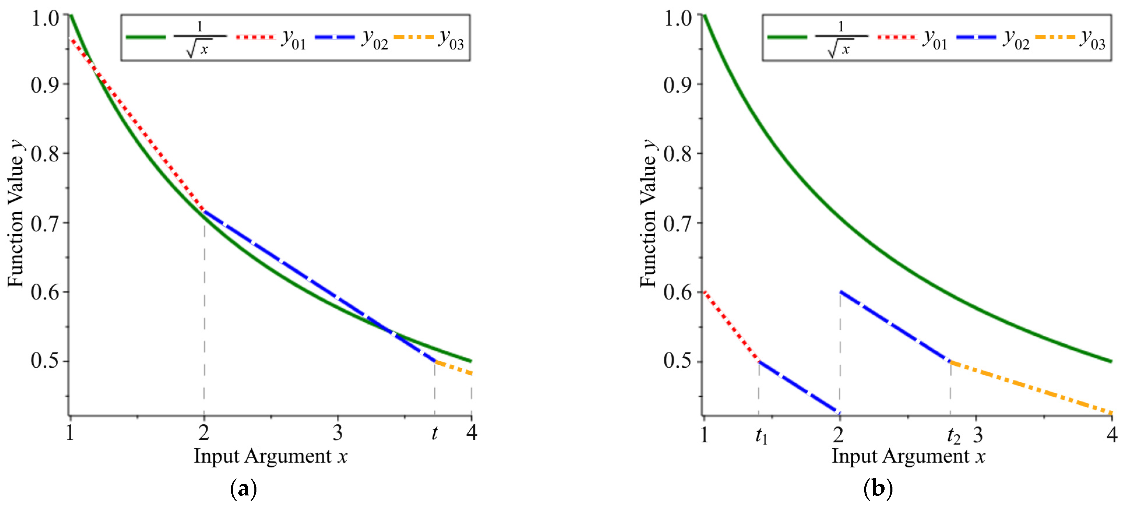
3. Method of Switching Magic Constants

The main idea of the proposed method is to split the interval $x\in [1, 4)$ of the initial approximation $y_0$ (see Figure 1a), on which it has different error values, into two parts—$x\in [1, 2)$ and $x\in [2, 4)$—and to perform an approximation of the reciprocal square root function separately in these subintervals. The variable $x$, as defined in Equation (2), then has different values in the last bit of the exponent $E_x$—zero in the first case and one in the second. We split the interval only for the initial approximation $y_0$—where the magic constant $R$ is used—and for the corresponding modified first iteration of the FISR method. As shown below, this technique allows us to reduce the maximum relative error of the algorithm after the first iteration by an order of magnitude compared to Algorithm 2 (RcpSqrt2).

Let us now consider this method in more detail. We require that, on the first and second parts of the interval $x\in [1, 2)$, the relative errors of two adjacent piecewise linear initial approximations $y_{01}$ and $y_{02}$ have the same scope—the same difference between the maximum and minimum values—as shown in Figure 2a. From this, it follows that the relative errors of the approximations $y_{01}$, $x\in [1, t_1)$ and $y_{02}$, $x\in [t_1, 2)$ have a similar symmetrical nature with respect to some common value at a point $x=t_1$. We will now find the value of the magic constant that gives the corresponding equations for $y_{01}$ and $y_{02}$. To do this, we write the analytical equations for the approximations $y_{01}$ and $y_{02}$ based on Equations (9)–(13) and the results of [28,29]:

$$y_{01}=-\frac{1}{4}x+\frac{1}{2}+\frac{1}{2}{m}_R+\frac{1}{4N_m}, x\in [1, t_1)$$

(14)

$$y_{02}=-\frac{1}{8}x+\frac{1}{2}+\frac{1}{4}{m}_R+\frac{1}{8N_m}, x\in [t_1, 2),$$

(15)

where, in this case,

$$t_1=2m_R+1/N_m.$$

(16)

Note also that the third linear approximation, which is not used in the result, has the form

$$y_{03}=-\frac{1}{16}x+\frac{3}{8}+\frac{1}{4}{m}_R+\frac{1}{8N_m}, x\in [2, 4).$$

(17)

Hence, the expressions for the relative errors are

$${\delta }_{01}=y_{01}\sqrt{x}-1=-\frac{1}{4}{x}^{3/2}+\frac{1}{2}{x}^{1/2}+\frac{1}{2}{x}^{1/2}{m}_R+\frac{1}{4N_m}{x}^{1/2}-1$$

(18)

$${\delta }_{02}=y_{02}\sqrt{x}-1=-\frac{1}{8}{x}^{3/2}+\frac{1}{2}{x}^{1/2}+\frac{1}{4}{x}^{1/2}{m}_R+\frac{1}{8N_m}{x}^{1/2}-1.$$

(19)

Having found the points of maxima and contact, we can determine the value of $m_R$:

$$m_R=0.70241439342498779296875$$

(20)

and the corresponding value of the magic constant $R$ for SP numbers:

$$R_1=0\mathrm{x}5\mathrm{ed}9\mathrm{e}8\mathrm{b}7.$$

(21)

Let us now examine the interval $x\in [2, 4)$. In the same way, we require that, for the second and third parts, the relative errors of two adjacent piecewise linear initial approximations $y_{02}$ and $y_{03}$ have the same scope (see Figure 2b). In this case,

$$y_{02}=-\frac{1}{8}x+\frac{3}{4}+\frac{1}{2}{m}_R+\frac{1}{4N_m}, x\in [2, t_2)$$

(22)

$$y_{03}=-\frac{1}{16}x+\frac{5}{8}+\frac{1}{4}{m}_R+\frac{1}{8N_m}, x\in [t_2, 4).$$

(23)

Note that, at the same time,

$$t_2=2+4m_R+2/N_m$$

(24)

and the first linear approximation, not relevant for the result, has the form:

$$y_{01}=-\frac{1}{4}x+1+\frac{1}{2}{m}_R+\frac{1}{4N_m}, x\in [1, 2).$$

(25)

Hence, we find that

$$m_R=0.20241439342498779296875$$

(26)

$$R_2=0\mathrm{x}5\mathrm{f}19\mathrm{e}8\mathrm{b}7.$$

(27)

As a result, the combined approach with magic constants $R_1$, (21), and $R_2$, (27), on two different subintervals gives us an opportunity to obtain the piecewise linear initial approximation $y_0$ on the interval $x\in [1, 4)$, as shown in Figure 1b. This can potentially offer a better approximation of the function $y=1/\sqrt{x}$, but only after some alignment (bias at each subinterval). For comparison, both of the magic constants used in the algorithms RcpSqrt1 and RcpSqrt2 give the initial approximation, as described in Equations (9)–(13) (see Figure 1a). Although the basic FISR method gives a much more accurate approximation at this stage, our method has four piecewise linear sections of the approximation $y_0$ rather than three, providing higher accuracy after the first iteration (see Figure 3). This trick is possible due to the modification of the first NR iteration at each of the subintervals. In other words, we align the corresponding errors of the initial approximation as described below.

For each subinterval, we modify the first NR iteration according to Equation (1) as follows:

$$y_1=k_1{y}_0(k_2-x{y}_0{y}_0),$$

(28)

where $k_1$ and $k_2$ are some FP constants that minimize the maximum relative error of the algorithm and depend on the value of the magic constant $R$. This modified iteration also involves four multiplications.

In order to determine the subinterval in the IEEE 754 format to which $x$ belongs—$x\in [1, 2)$ or $x\in [2, 4)$—we check the least significant bit (LSB) of the biased exponent

$$e_x=E_x+bias.$$

(29)

In the SW implementation, we apply a bit mask to $x$. Then, we choose the magic constant and the first modified NR iteration that correspond to this value. We call this technique the method of switching magic constants or the dynamic constants (DC) method.

It should be noted that this method can be generalized to more constants. In this case, each of the indicated subintervals is further divided into two, four, eight, etc., equal parts depending on the value of one or more most significant bits of the fractional part of the mantissa $m_x$, and the bit mask is changed accordingly. However, in general, it cannot be guaranteed that such a partition will significantly improve the accuracy of the algorithm in all the parts; therefore, some parts should be divided further.

The general structure of the proposed SW RcpSqrt3 algorithms for two magic constants, with the modified FISR initial approximation $y_0$, the first modified iteration (28), and a branching statement (comparison with zero) using bit masking (bitwise AND), is shown in Template 1. Here, the input argument $x$ has type <fp_type>, which can be float, double, etc., and <int_type> is the corresponding integer type. The names of the algorithms for the reciprocal square root are constructed according to the template, as follows: RcpSqrt3<iter><version><fp_type_abbr>, where <iter> is the number of iterations used in the algorithm, <version> is an optional index, and <fp_type_abbr> indicates the required FP data type. This also applies to the square root calculation algorithms, which we denote as Sqrt3. The parameters $R_1$ and $R_2$ are integer magic constants; $k_{11}$, $k_{12}$, $k_{21}$, and $k_{22}$ are FP constants, which are defined later. When implemented in HW, in this case, a small 1-bit LUT can be used to choose appropriate values for the parameters $R$, $k_1$, and $k_2$.

Template 1. Basic structure of the proposed DC algorithms for the reciprocal square root.

1: <fp_type> RcpSqrt3<iter><version><fp_type_abbr> [       <int_type> $R_1$, <int_type> $R_2$,       <fp_type> $k_{11}$, <fp_type> $k_{12}$,       <fp_type> $k_{21}$, <fp_type> $k_{22}$] (<fp_type> x)

2: {

3:  <int_type> i = *(<int_type>*)&x;   // x—input argument

4:  <int_type> k = i & <ex_mask>;    // binary mask on the LSB of $e_x$

5:  <fp_type> y;

6:  if (k != 0) {

7:   i = $R_1$ – (i >> 1);       //$R_1$—first magic constant

8:   y = *(<fp_type>*)&i;       // approximation $y_0$

9:   y = $k_{11}$*y*($k_{12}$ – x*y*y);     // first modified NR iteration

10:  } else {

11:   i = $R_2$–(i >> 1);        //$R_2$—second magic constant

12:   y = *(<fp_type>*)&i;      // approximation $y_0$

13:   y = $k_{21}$*y*($k_{22}$ – x*y*y);     // first modified NR iteration

14:  }               // DC initial approximation $y_1$

15:   …              // subsequent NR or modified NR iterations

16:  return y;            // output $y_{<iter>}$

17: }

The proposed method can be thought of as a relatively accurate and fast initial guess $y_1$—the DC initial approximation—for other iterative algorithms (see Template 1, lines 14–16). In this paper, we consider modified NR iterations written in a special form, with combined multiply–add operations.

Furthermore, in this section, we present final (ready-to-use) codes for the proposed algorithms in C/C++ and give their errors (accuracy results).

Note that—when determining the relative errors of these algorithms—giving here an example for the reciprocal square root function—we used the following notation for the upper and lower limits of the maximum relative error, respectively:

$${\delta }_{\max }^{+}=\underset{x\in [1, 4)}{\max }(y\sqrt{x}-1)$$

(30)

$${\delta }_{\max }^{-}=\underset{x\in [1, 4)}{\min }(y\sqrt{x}-1).$$

(31)

Alternatively, without taking into account the sign of the error, the maximum relative error was determined using the formula

$${\delta }_{\max }=\underset{x\in [1, 4)}{\max }|y\sqrt{x}-1|=\max \left\{\right|{\delta }_{\max }^{-}|, |{\delta }_{\max }^{+}\left|\right\}.$$

(32)

To iterate over all possible float values in the interval $x\in [1, 4)$, we used the $\mathrm{nextafterf} (x, d)$ function from the cmath library. For the case of type double, we traversed this interval with a small step—about $1 \times {10}^{-12}$. As a reference implementation, we used a higher-precision $\mathrm{sqrt} (x)$ or $\mathrm{sqrtl} (x)$ function from this library. The number of accurate digits in the result—accuracy of the algorithm—was determined in bits by the formula

$$\alpha =-{\log }_2({\delta }_{\max }).$$

(33)

Error measurements for the algorithms were performed on a quad-core Intel Core i7-7700HQ processor using a GNU compiler (GCC 4.9.2) for C++ on a Windows 10 (64-bit) operating system with options as follows: -std = c++11 -Os -ffp-contract = on -mfma.

3.1. SP Reciprocal Square Root (RcpSqrt3 for Float)

3.1.1. One Iteration—The DC Initial Approximation

For the interval $x\in [1, 2)$ and the theoretically determined magic constant for SP $R_1$, (21), the unknown theoretical coefficients $k_1$ and $k_2$ in Equation (28) that minimize the maximum relative error ${\delta }_{\max }$ after the first iteration are

$$k_{11}=2.3312425, k_{12}=1.07497365.$$

(34)

Similarly, for $x\in [2, 4)$ and the magic constant $R_2$, (27),

$$k_{21}=0.8242186, k_{22}=2.1499476.$$

(35)

An implementation of the algorithm with these parameters shows the maxima of the relative errors

$${\delta }_{\max }^{+}=7.462402 \times {10}^{-5} \hspace{1em}{\delta }_{\max }^{-}=-7.459646 \times {10}^{-5}.$$

(36)

If a computing platform has a fast HW or SW implementation of the fused multiply–add ($\mathrm{fma}$) function, $\mathrm{fma} (a, b, c)=ab+c$, then in Template 1, iteration (28) can be written as

$$y_1=k_1{y}_0\mathrm{fma} (-x, y_0{y}_0, k_2).$$

(37)

On some platforms, when implemented in HW, this function can increase both the speed and the accuracy of the algorithms. The $\mathrm{fma}$ operation has fewer roundings and much higher precision for the internal calculations. In the remainder of this section, unless otherwise specified, we use the $\mathrm{fma}$ function in all algorithms.

Taking into account the rounding errors and the issue of the best practical representation of the theoretical parameters in the target SP FP format, we can improve our theoretical parameters $R_1$, $R_2$, $k_{11}$, $k_{12}$, $k_{21}$, and $k_{22}$ (given in (21), (27), (34), (35)). A brute force optimization method was used in a certain neighborhood of the defined theoretical parameters to minimize the maximum relative error of the algorithm on each of the subintervals. This approach also includes elements of randomized multidimensional greedy optimization for coarse search. In this case, three parameters $R$, $k_1$, and $k_2$ are optimized simultaneously. The method is described in more detail in [38].

Algorithm 3 below gives the proposed improved RcpSqrt31f algorithm for SP numbers with one iteration. This algorithm provides slightly lower values for the maximum relative errors:

$${\delta }_{\max }^{+}=7.459289 \times {10}^{-5} \hspace{1em}{\delta }_{\max }^{-}=-7.450387 \times {10}^{-5}.$$

(38)

Algorithm 3. Proposed RcpSqrt31f algorithm (DC initial approximation).

1: float RcpSqrt31f (float x)

2: {

3:  int i = *(int*)&x;

4:  int k = i & 0x00800000;

5:  float y;

6:  if (k != 0) {

7:   i = 0x5ed9e91f – (i >> 1);

8:   y = *(float*)&i;

9:   y = 2.33124256f*y*fmaf(−x, y*y, 1.0749737f);

10:  } else {

11:   i = 0x5f19e8fc – (i >> 1);

12:   y = *(float*)&i;

13:   y = 0.824218631f*y*fmaf(−x, y*y, 2.1499474f);

14:  }

15:  return y;

16: }

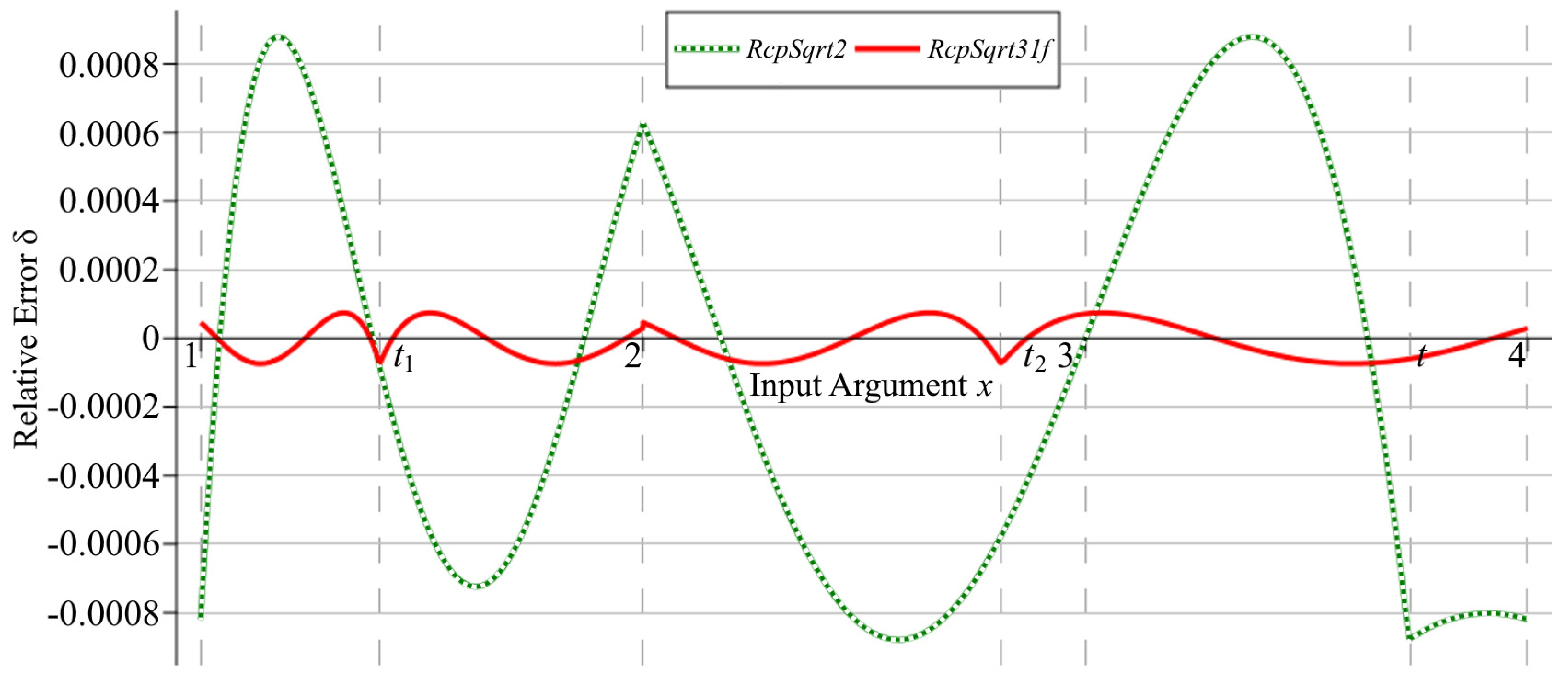
Graphs of the relative errors of the RcpSqrt2 and RcpSqrt31f algorithms after the first iteration are shown in Figure 3. Numerical experiments show that the maximum relative error of the RcpSqrt2 algorithm after the first iteration is ${\delta }_{\max }=8.792 \times {10}^{-4}$, corresponding to 10.15 correct bits of the result, and, for our algorithm, from (38), ${\delta }_{\max }=7.459 \times {10}^{-5}$, providing 13.71 correct bits. Consequently, the error is reduced by a factor of more than 11.7.

3.1.2. Two Iterations

To increase the accuracy of the RcpSqrt31f algorithm described above, it is possible to apply an additional NR iteration over the entire range $x\in [1, 4)$. The second iteration is common to both subintervals, uses the $\mathrm{fma}$ function, and has the specific form

$$\begin{gathered} c_1=x{y}_1 \\ {r}_1=\mathrm{fma} (y_1, -c_1, k_3) \\ {y}_2=\mathrm{fma} (k_4{y}_1, r_1, y_1), \end{gathered}$$

(39)

where, in this case, for the SP version,

$$k_3=1.0, k_4=0.5,$$

(40)

which corresponds to the classical Equation (1). The use of the $\mathrm{fma}$ function in the second iteration in the form given in (39) is important, since it greatly improves the accuracy of the algorithm at the final stage of the calculations. However, compared to the RcpSqrt1 and RcpSqrt2 algorithms, it has four multiplications rather than three in the second iteration (a further addition is also hidden inside $\mathrm{fma}$). If we write the second iteration in the same way as in Equation (37), we only get 22.68 bits of accuracy (${\delta }_{\max }=1.492 \times {10}^{-7}$). A full C/C++ code for two NR iterations is given in Algorithm 4. Here, we also make some corrections to the values of $R_1$, $R_2$, $k_{11}$, $k_{12}$, $k_{21}$, and $k_{22}$ (given in (21), (27), (34), (35)) to minimize the maximum errors of the complete RcpSqrt32f algorithm, in a similar way to the approach described in Section 3.1.1. An alternative would be to modify the values of $k_3$ and $k_4$, although this is less effective for type float.

Algorithm 4. Proposed RcpSqrt32f algorithm.

1: float RcpSqrt32f (float x)

2: {

3:  float y = RcpSqrt31f [        $R_1$= 0x5ed9dbc6, $R_2$= 0x5f19d200,        $k_{11}$= 2.33124018f, $k_{12}$= 1.07497406f,        $k_{21}$= 0.824212492f, $k_{22}$= 2.14996147f] (x);

4:  float c = x*y;

5:  float r = fmaf(y, −c, 1.0f);

6:  y = fmaf(0.5f*y, r, y);

7:  return y;

8: }

The final RcpSqrt32f algorithm has errors

$${\delta }_{\max }^{+}=7.362378 \times {10}^{-8} \hspace{1em}{\delta }_{\max }^{-}=-7.754203 \times {10}^{-8},$$

(41)

or 23.62 correct bits of the result out of a possible $p+1=24$ for float numbers. Note that, when this algorithm has the same constants for the initial approximation as in Algorithm 3—RcpSqrt31f plus classic NR in the form given in (39), (40)—it has an error ${\delta }_{\max }=8.038 \times {10}^{-8}$.

3.2. SP Square Root (Sqrt3 for Float)

We now turn to the square root calculation algorithms to find an approximation for $y=\sqrt{x}$ in SP. As noted in Section 1, these algorithms can easily be obtained from those previously described, simply by multiplying the result by the value of the input argument $x$. However, this involves an additional multiplication operation, and in our algorithms, in most cases, this can be avoided by modifying the last iteration.

3.2.1. One Iteration—The DC Initial Approximation

For one iteration, we make a substitution $c_0=x{y}_0$ in Equation (37). Then, the first iteration for the square root at each subinterval is written as

$$\begin{gathered} c_0=x{y}_0 \\ {y}_1=k_1{c}_0\mathrm{fma} (y_0, -c_0, k_2). \end{gathered}$$

(42)

Algorithm 5 provides the final code for Sqrt31f with optimized constants. After the first iteration, the algorithm has errors

$${\delta }_{\max }^{+}=7.450372 \times {10}^{-5} \hspace{1em}{\delta }_{\max }^{-}=-7.451108 \times {10}^{-5},$$

(43)

and hence it has the same level of error as the RcpSqrt31f algorithm. In addition, in Algorithm 5, the same constants can be used as in RcpSqrt31f (${\delta }_{\max }=7.46 \times {10}^{-5}$).

Algorithm 5. Proposed Sqrt31f algorithm (DC initial approximation).

1: float Sqrt31f (float x)

2: {

3:  int i = *(int*)&x;

4:  int k = i & 0x00800000;

5:  float y;

6:  if (k != 0) {

7:   i = 0x5ed9e893 – (i >> 1);

8:   y = *(float*)&i;

9:   float c = x*y;

10:   y = 2.33130789f*c*fmaf(y, −c, 1.07495356f);

11:  } else {

12:   i = 0x5f19e8fd – (i >> 1);

13:   y = *(float*)&i;

14:   float c = x*y;

15:   y = 0.82421863f*c*fmaf(y, −c, 2.1499474f);

16:  }

17:  return y;

18: }

3.2.2. Two Iterations

When we use two NR iterations to calculate the square root function (Sqrt32f), the structure of the algorithm does not change compared to RcpSqrt32f, and we need only modify the second iteration (see Algorithm 6, line 6). This algorithm has slightly lower accuracy than RcpSqrt32f, with

$${\delta }_{\max }^{+}=8.757966 \times {10}^{-8} \hspace{1em}{\delta }_{\max }^{-}=-9.037992 \times {10}^{-8}.$$

(44)

This corresponds to 23.4 exact bits—${\delta }_{\max }=9.216 \times {10}^{-8}$, if we do not change the constants of the DC initial approximation, i.e., the RcpSqrt31f algorithm.

Algorithm 6. Proposed Sqrt32f algorithm.

1: float Sqrt32f (float x)

2: {

3:  float y = RcpSqrt31f [       $R_1$= 0x5ed9d098, $R_2$= 0x5f19d352,       $k_{11}$= 2.33139729f, $k_{12}$= 1.07492042f,       $k_{21}$= 0.82420468f, $k_{22}$= 2.14996147f] (x);

4:  float c = x*y;

5:  float r = fmaf(y, −c, 1.0f);

6:  y = fmaf(0.5f*c, r, c);    // modified

7:  return y;

8: }

3.3. DP Reciprocal Square Root (RcpSqrt3 for Double)

3.3.1. One Iteration—The DC Initial Approximation

Similarly, this method can be applied to FP numbers of DP. In this case, the theoretically determined magic constants based on (20) and (26) are

$$R_1=0\mathrm{x}5\mathrm{fdb}3\mathrm{d}16\mathrm{dd}72\mathrm{c}671$$

(45)

$$R_2=0\mathrm{x}5\mathrm{fe}33\mathrm{d}16\mathrm{dd}72\mathrm{c}671.$$

(46)

The overall structure of the algorithm does not change (see Template 1), and only the data types used in the calculations are modified compared to the RcpSqrt31f algorithm. The corresponding algorithm for DP is given in Algorithm 7. Here, the parameters $R_1$, $R_2$, $k_{11}$, $k_{12}$, $k_{21}$, and $k_{22}$ are 64-bit constants after optimization. Note that the specified improved constants can be quite different from the theoretical ones according to the practical optimization method used. This has the following aligned maxima in the relative errors:

$${\delta }_{\max }^{+}=7.437897 \times {10}^{-5} \hspace{1em}{\delta }_{\max }^{-}=-7.437897 \times {10}^{-5},$$

(47)

corresponding to an accuracy of 13.71 bits.

Algorithm 7. Proposed RcpSqrt31d algorithm (DC initial approximation).

1: double RcpSqrt31d (double x)

2: {

3:  uint64_t i = *(uint64_t*)&x;

4:  uint64_t k = i & 0x0010000000000000;

5:  double y;

6:  if (k != 0) {

7:   i = 0x5fdb3d20982e5432 – (i >> 1);

8:   y = *(double*)&i;

9:   y = 2.331242396766632*y*fma(−x, y*y, 1.074973693828754);

10:  } else {

11:   i = 0x5fe33d209e450c1b – (i >> 1);

12:   y = *(double*)&i;

13:   y = 0.824218612684476826*y*fma(−x, y*y, 2.14994745900706619);

14:  }

15:  return y;

16: }

3.3.2. Two Iterations

The RcpSqrt32d algorithm for finding the DP reciprocal square root with two iterations is shown in Algorithm 8. Note that, here, we use the same constants for the DC initial approximation as in the RcpSqrt31d algorithm. This algorithm has a second iteration in the form of (39), with changes in the following two constants:

$$k_3=1.000000008298416, k_4=0.50000000057372.$$

(48)

The maximum relative errors of this algorithm are

$${\delta }_{\max }^{+}=4.149208 \times {10}^{-9} \hspace{1em}{\delta }_{\max }^{-}=-4.149157 \times {10}^{-9}$$

(49)

(27.84 correct bits), in contrast to ${\delta }_{\max }=7.75 \times {10}^{-8}$ for SP numbers (see (41)). The modification of the last NR iteration in the form (39), (48) allows us to increase the accuracy of the algorithm from 26.84 bits in the case of a classic iteration to 27.84 bits.

Algorithm 8. Proposed RcpSqrt32d algorithm.

1: double RcpSqrt32d (double x)

2: {

3:  double y = RcpSqrt31d (x);

4:  double c = x*y;

5:  double r = fma(y, −c, 1.000000008298416);

6:  y = fma(0.50000000057372*y, r, y);

7:  return y;

8: }

3.3.3. Three Iterations

For three iterations in DP, we present two versions of the algorithm: one with fewer multiplication operations (RcpSqrt331d) and one with higher accuracy (RcpSqrt332d). The complete RcpSqrt331d algorithm is given in Algorithm 9. The errors of this algorithm have the following boundaries:

$${\delta }_{\max }^{+}=1.603535 \times {10}^{-16} \hspace{1em}{\delta }_{\max }^{-}= -1.826339 \times {10}^{-16}$$

(50)

(52.28 correct bits). Here, we have made the substitution $mxhalf=-0.5x$ (line 4) in a similar way as in RcpSqrt1 and RcpSqrt2. This allows us to avoid one multiplication and also to use that substitution in classic or modified NR iterations. In this case, the second and third iterations have the following form:

$$\begin{gathered} mxhalf=-0.5x \\ {y}_2=y_1\mathrm{fma} (mxhalf, y_1{y}_1, k_3) \end{gathered}$$

(51)

$$\begin{gathered} r_2=\mathrm{fma} (mxhalf, y_2{y}_2, k_4) \\ {y}_3=\mathrm{fma} (y_2, r_2, y_2), \end{gathered}$$

(52)

where

$$k_3=1.5000000034937999, k_4=0.5.$$

(53)

If we do not change the initial approximation constants in Algorithm 9—RcpSqrt31d plus modified and classic NR iterations in the form (51)–(53)—we obtain 52.23 bits of accuracy (${\delta }_{\max }=1.898 \times {10}^{-16}$).

Algorithm 9. Proposed RcpSqrt331d (faster) algorithm.

1: double RcpSqrt331d (double x)

2: {

3:  double y = RcpSqrt31d [        $R_1$= 0x5fdb3d14170034b6, $R_2$= 0x5fe33d18a2b9ef5f,        $k_{11}$= 2.33124735553421569, $k_{12}$= 1.07497362654295614,        $k_{21}$= 0.82421942523718461, $k_{22}$= 2.1499494964450325] (x);

4:  double mxhalf = −0.5*x;

5:  y = y*fma(mxhalf, y*y, 1.5000000034937999);

6:  double r = fma(mxhalf, y*y, 0.5);

7:  y = fma(y, r, y);

8:  return y;

9: }

On the other hand, if we do not make this substitution and write the last iteration using $c_2=x{y}_2$, we obtain an algorithm RcpSqrt332d that contains one more multiplication and an additional coefficient in the last iteration. In this case, the last two iterations of the algorithm are (see Algorithm 10, lines 4–7)

$$y_2=y_1\mathrm{fma} (k_{3}x, y_1{y}_1, k_4)$$

(54)

$$\begin{gathered} c_2=x{y}_2 \\ {r}_2=\mathrm{fma} (y_2, -c_2, 1.0) \\ {y}_3=\mathrm{fma} (k_5{y}_2, r_2, y_2), \end{gathered}$$

(55)

where

$$k_3=-0.5000000000724769, k_4=1.50000000394948985, k_5=0.50000000001394973.$$

(56)

Compared to RcpSqrt331d, the RcpSqrt332d algorithm has lower maximum relative errors after the third iteration,

$${\delta }_{\max }^{+}=1.363926 \times {10}^{-16} \hspace{1em}{\delta }_{\max }^{-}=-1.606246 \times {10}^{-16}$$

(57)

(52.47 exact bits). Note that the other alternatives to this algorithm—RcpSqrt31d plus two modified NR in the form (54)–(56) and RcpSqrt32d plus classic NR in the form given in (55), where $k_5=0.5$—are slightly less accurate (52.44 correct bits).

Algorithm 10. Proposed RcpSqrt332d (higher accuracy) algorithm.

1: double RcpSqrt332d (double x)

2: {

3:  double y = RcpSqrt31d [        $R_1$= 0x5fdb3d15bd0ca57e, $R_2$= 0x5fe33d190934572f,        $k_{11}$= 2.3312432409377752, $k_{12}$= 1.0749736243940957,        $k_{21}$= 0.824218531163110613, $k_{22}$= 2.1499488934465218] (x);

4:  y = y*fma(−0.5000000000724769*x, y*y, 1.50000000394948985);

5:  double c = x*y;

6:  double r = fma(y, −c, 1.0);

7:  y = fma(0.50000000001394973*y, r, y);

8:  return y;

9: }

3.4. DP Square Root (Sqrt3 for Double)

3.4.1. One and Two Iterations

In the same way as for the type float and reciprocal square root, we construct algorithms for the square root in DP using one and two iterations. These are based on the RcpSqrt31d and RcpSqrt32d algorithms. The errors of these algorithms are close to those of the reciprocal square root (see (47) and (49)).

3.4.2. Three Iterations

For the algorithm with three iterations, we cannot avoid the additional multiplication, as we did in the RcpSqrt331d algorithm described above. Hence, we present only an algorithm that has four multiplications in the third iteration—including $\mathrm{fma}$ operations. It is based on RcpSqrt332d, in which the last iteration (55) is modified for the square root calculation, and the corresponding parameters are optimized, as shown in Algorithm 11. After the third iteration, this algorithm has errors of

$${\delta }_{\max }^{+}=1.66425 \times {10}^{-16} \hspace{1em}{\delta }_{\max }^{-}=-1.847481 \times {10}^{-16}$$

(58)

(52.27 correct bits). If we do not modify the constants of the DC initial approximation in Algorithm 11, the accuracy is 52.25 bits. The algorithm based on RcpSqrt32d—RcpSqrt32d plus a modified for the square root version of the classic NR iteration in a special form—has 52.23 bits of accuracy.

Algorithm 11. Proposed Sqrt33d algorithm.

1: double Sqrt33d (double x)

2: {

3:  double y = RcpSqrt31d [        $R_1$= 0x5fdb3d20dba7bd3c, $R_2$= 0x5fe33d165ce48760,        $k_{11}$= 2.3312471012384104, $k_{12}$= 1.074974060752685,        $k_{21}$= 0.82421918338542632, $k_{22}$= 2.1499482562039667] (x);

4:  y = y*fma(−0.50000000010988821*x, y*y, 1.5000000038700285);

5:  double c = x*y;

6:  double r = fma(y, −c, 1.0);

7:  y = fma(0.50000000001104072*c, r, c);    // modified

8:  return y;

9: }

4. Experimental Results and Discussion

Performance testing of these algorithms was conducted on a Raspberry Pi 3 Model B mini-computer and an ESP-WROOM-32 microcontroller. The Raspberry Pi is based on a quad-core 64-bit SoC Broadcom BCM2837 (1.2 GHz, 1 Gb RAM) with an ARM Cortex-A53 processor [6]. We used the GNU compiler (GCC 6.3.0) for Raspbian OS (32-bit) with the following compilation options: -std = c++11 -Os -ffp-contract = on -mfpu = neon-fp-armv8 -mcpu = cortex-a53. The 32-bit Wi-Fi module ESP-WROOM-32 (ESP-32) from Espressif Systems has two low-power Xtensa microprocessors (240 MHz, 520 Kb RAM) [39]. The microcontroller was programmed via the Arduino IDE (GCC 5.2.0) with the following compilation parameters: -std = gnu++11 -Os -ffp-contract = fast. The speed (latency) of the algorithms was measured using the chrono C++ library. Depending on the platform, at least 200 tests were run in which functions were called sequentially in a single thread (core), a million or more times. The average results of these performance tests are given here.

It should be noted that, although we chose C++ to implement the algorithms, it is worth using an inline assembly code for more efficient and better performance optimization on each specific platform. However, the chosen compilation options gave a fairly effective fast code optimization and allowed us to automatically translate the $\mathrm{fmaf} (a, b, c)$ and $\mathrm{fma} (a, b, c)$ C++ functions into the corresponding HW instructions; for the microcontroller, the compiler may even automatically replace successive multiplication and addition/subtraction operations of SP with the corresponding $\mathrm{fma}$ HW instructions (the -ffp-contract = fast option, which enables FP expression contraction).

The accuracy and latency measurements for the reciprocal square root ($y=1/\sqrt{x}$) and square root ($y=\sqrt{x}$) functions, in both SP and DP, are summarized in

Table 1. Comparison of different methods for calculating the reciprocal square root and square root for single (SP) and double (DP) precision on the Raspberry Pi mini-computer and the ESP-32 microcontroller.

Function	Data Type	Method	Relative Error		Accuracy (Bits)	Latency (ns)
			${\delta }_{\mathbf{max}}^{+}$	${\delta }_{\mathbf{max}}^{-}$		RP 3	ESP-32
$1/\sqrt{x}$	Float	1.0f/sqrtf (x)	8.9407 × 10−8	−8.9348 × 10−8	23.42	178.6	–
		divf (1.0f, sqrtf (x))	8.9407 × 10−8	−8.9348 × 10−8	23.42	–	797.3
		Walczyk: 1
		1 iter.	8.7919 × 10−4	−8.7921 × 10−4	10.15	25.9	234.9
		2 iter.	6.7893 × 10−7	−6.4727 × 10−7	20.49	40.2	281.1
		DC: 1
		1 iter. (RcpSqrt31f)	7.4593 × 10−5	−7.4504 × 10−5	13.71	28.5	248.0
		2 iter. (RcpSqrt32f)	7.3624 × 10−8	−7.7542 × 10−8	23.62	52.2	340.3
		FRSQRTE 2	3.2768 × 10−3	−3.0354 × 10−3	8.25	19.3	–
		FRSQRTE + FRSQRTS: 2
		1 iter.	1.3127 × 10−7	−1.6183 × 10−5	15.92	40.2	–
		2 iter.	1.6064 × 10−7	−1.5772 × 10−7	22.6	60.4	–
	Double	1.0/sqrt (x)	1.6653 × 10−16	−1.6653 × 10−16	52.42	199.2	–
		div (1.0, sqrt (x))	1.6653 × 10−16	−1.6653 × 10−16	52.42	–	6984.8
		DC: 1
		1 iter. (RcpSqrt31d)	7.4379 × 10−5	−7.4379 × 10−5	13.72	28.5	2744.1
		2 iter. (RcpSqrt32d)	4.1492 × 10−9	−4.1492 × 10−9	27.84	51.1	5128.4
		3 iter. (RcpSqrt331d)	1.6035 × 10−16	−1.8263 × 10−16	52.28	56.1	6828.2
		3 iter. (RcpSqrt332d)	1.3639 × 10−16	−1.6062 × 10−16	52.47	64.5	7237.8
$\sqrt{x}$	Float	sqrtf (x)	5.9565 × 10−8	−5.9605 × 10−8	24.00	172.1	604.3
		Walczyk: 1, 3
		1 iter.	8.7919 × 10−4	−8.7919 × 10−4	10.15	28.4	234.9
		2 iter.	6.8215 × 10−7	−6.4493 × 10−7	20.48	43.4	302.0
		DC: 1
		1 iter. (Sqrt31f)	7.4504 × 10−5	−7.4511 × 10−5	13.71	27.5	264.8
		2 iter. (Sqrt32f)	8.7580 × 10−8	−9.0380 × 10−8	23.40	47.5	340.3
	Double	sqrt (x)	1.1102 × 10−16	−1.1102 × 10−16	53.00	187.8	4403.3
		DC: 1
		1 iter.	7.4379 × 10−5	−7.4379 × 10−5	13.72	34.1	2650.4
		2 iter.	4.1492 × 10−9	−4.1492 × 10−9	27.85	46.8	5047.6
		3 iter. (Sqrt33d)	1.6643 × 10−16	−1.8475 × 10−16	52.27	59.3	7151.9

¹ Implemented with HW $\mathrm{fma}$ operations (except for DP on ESP-32, where SW $\mathrm{fma}$ is used). ² HW instructions in Raspberry Pi (the estimate FRSQRTE instruction is based on a LUT and the FRSQRTS instruction is used to perform the classic NR iteration). ³ Modified for the square root calculation.

. In this table, we consider the various methods available on the mini-computer and microcontroller, including the cmath SW library functions ($\mathrm{sqrtf} (x)$ and $\mathrm{sqrt} (x)$) [5] and the built-in NEON instructions (FRSQRTE and FRSQRTS) [11] for an approximate calculation of the reciprocal square root in Raspberry Pi using NR iterations. We also compare the method of Walczyk et al. (the RcpSqrt2 algorithm) [29], its modification for calculation of the square root, and the proposed method of switching magic constants (the DC algorithms from Section 3). Here, both the Walczyk et al. and the DC algorithms are implemented using the $\mathrm{fma}$ function.

Even on platforms that do not have special HW instructions for the square root and reciprocal square root (either approximate or with full accuracy), such as ESP-32, the C++ function $\mathrm{sqrt} (x)$ is available for both SP and DP numbers. Modern platforms, such as Intel or ARM, may also have the appropriate hardware FSQRT instructions. These are IEEE-compliant and ensure the full accuracy of the result (see the $\mathrm{sqrtf} (x)$ and $\mathrm{sqrt} (x)$ functions in Table 1).

Looking at the results from Table 1, it becomes obvious that the main feature of our proposed DC algorithms for the float and double types is that the algorithms RcpSqrt32f, Sqrt32f, RcpSqrt331d, RcpSqrt332d, and Sqrt33d allow the result to be obtained up to the last bit—although the 24th and 53rd bits may be wrong. At the same time, the RcpSqrt32f and RcpSqrt332d algorithms for the reciprocal square root have somewhat higher accuracy than the naive method using division.

All the platforms tested have HW-implemented multiplication, addition, and $\mathrm{fma}$ operations for FP numbers of SP and, except for ESP-32, DP [10,11,12]. Since the ESP microcontroller is a 32-bit system, all DP operations are performed by SW. Note that it also does not have a division instruction in SP [12], meaning that the latency of the corresponding operations is much higher.

As shown in Table 1, the proposed algorithms give significantly better performance than the library functions on the Raspberry Pi, from 3.17 to 3.62 times faster, and for SP numbers on ESP-32, 2.34 times faster for the reciprocal square root and approximately 1.78 times faster than the $\mathrm{sqrtf} (x)$ function. At the same time, on the microcontroller with the SW implementation of DP $\mathrm{fma}$, the RcpSqrt331d algorithm is a little faster than the naive method using the $\mathrm{sqrt} (x)$ function, but has slightly lower accuracy. The RcpSqrt332d algorithm, in contrast, has higher accuracy, but worse performance. The proposed algorithms are also not efficient on ESP-32 for calculating the square root of DP numbers (in contrast to the Raspberry Pi). However, in some cases, it is possible to improve the performance of the algorithms in DP if fewer $\mathrm{fma}$ functions are used in the code, as shown later (see also [26] for more details).

In ARM with NEON technology [11], the HW SP instructions FRSQRTE and FRSQRTS, for which the corresponding intrinsics are $\mathrm{vrsqrte}\_\mathrm{f}32$ and $\mathrm{vrsqrts}\_\mathrm{f}32$, can be used to calculate a fast approximation of the reciprocal square root function and to perform the classical NR iteration (step), respectively. The FRSQRTE instruction is based on a LUT and gives 8.25 correct bits of the result (our DC initial approximation gives 13.71 bits). A combination of these instructions in the Raspberry Pi gives poorer accuracy and latency results than the RcpSqrt32f algorithm (see Table 1). It should also be noted that the HW FSQRT and 64-bit FRSQRTE instructions of the ARMv8 (AArch64) architecture are not available on the Raspberry Pi for the specified official 32-bit OS [11].

In order to ensure a fair comparison between the proposed algorithms and other advanced FISR-based methods, we also implemented an algorithm proposed by Walczyk et al. [29] in a specific form using the $\mathrm{fma}$ functions. This allowed us to strike a better compromise between accuracy and speed compared to the original RcpSqrt2 algorithm (see Table 1). For the square root calculation, we used the same method that we suggest for the DC algorithms. The results show that, although these algorithms are faster, their accuracy is much lower.

A comparison of the FISR-based algorithms that also provide 23 exact bits for a float and 52 exact bits for a double is given in

Table 2. Comparison of different FISR-based methods for calculating the SP reciprocal square root with high accuracy.

Method	Number of Operations									Accuracy (Bits)
	FP Fma 1	FP Mult	FP Add/Sub 2	FP–Int Transl 3	Int Add/Sub	Int Comp	Bit AND	Bit Shift	Total
Walczyk (1 iter.)	–	4	1	2	1	–	–	1	9	10.15
TMC (1 iter.)	–	3 (−1)	1	3 (+1)	2 (+1)	–	–	1	10 (+1)	10.59
Ho2 (1 iter.)	–	5 (+1)	2 (+1)	2	1	–	–	1	11 (+2)	15.63
DC (1 iter.)	–	4	1	2	1	1 (+1)	1 (+1)	1	11 (+2)	13.71
Walczyk (3 iter.)	2	8	2	2	1	–	–	1	16	23.42
TMC (2 iter.)	3 (+1)	5 (−3)	1 (−1)	3 (+1)	2 (+1)	–	–	1	15 (−1)	23.47
Ho2 (2 iter.)	2	7 (−1)	2	2	1	–	–	1	15 (−1)	23.69
DC (2 iter.)	2	6 (−2)	1 (−1)	2	1	1 (+1)	1 (+1)	1	15 (−1)	23.62

¹ The $\mathrm{fma}$ operation can be replaced with a combination of multiplication and addition/subtraction operations, but this can drastically affect the accuracy. ² Each FP addition/subtraction can be combined with an adjacent multiplication in the $\mathrm{fma}$ operation. ³ Transformation $\iota \left(x\right)$ or inverse transformation $\mathsf{\phi } \left(i\right)$.

for SP numbers. Note that, here, TMC denotes the method of two magic constants [26] and Ho2 denotes the approach based on the second-order Householder’s method [32] for the reciprocal square root. The relative performance of the proposed algorithms depends on the operations used, their sequence, and the characteristics of the platform. For example, the RcpSqrt32f (Algorithm 4) and InvSqrt5 [32] (Section VI) algorithms are fairly efficient on ESP-32 for SP numbers. However, to the best of our knowledge, the DC initial approximation is the only FISR-based method with one NR iteration—four multiplications and one subtraction—that provides 13 correct bits of the result for the square root and reciprocal square root functions. It can be implemented on FPGAs using a small LUT, and only one bit of the input argument (LSB of the exponent) needs to be controlled.

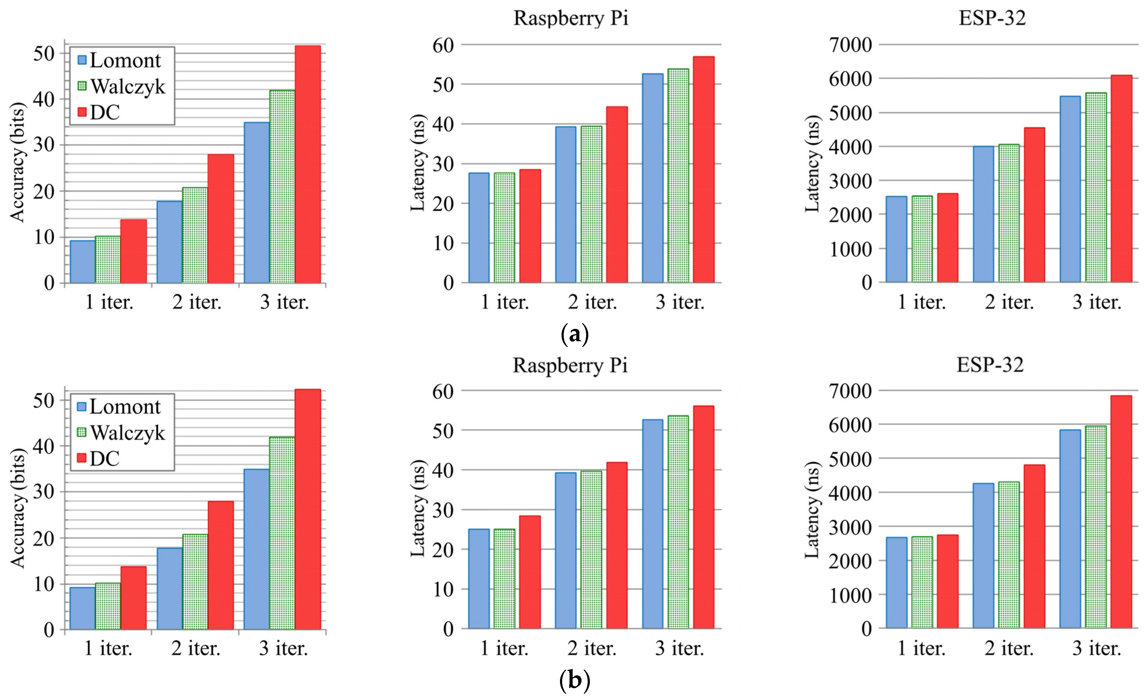
Figure 4 shows the results of a comparison of the Lomont [8,25], Walczyk et al. [29], and switching magic constants (DC) methods after each iteration for DP numbers—with and without the use of the $\mathrm{fma}$ operations. Here, we consider different ways of implementing NR iterations using the $\mathrm{fma}$ functions. As shown by the graphs, the accuracy is almost the same in both cases, with the sole exception of three iterations. The proposed DC algorithm (RcpSqrt331d), in most cases, has slower performance on the platforms considered here than the Lomont and Walczyk et al. algorithms (except perhaps one iteration), but is significantly superior in terms of accuracy. It allows us to obtain highly accurate results for the square root and reciprocal square root calculations for DP numbers by the third iteration. Note that, when the $\mathrm{fma}$ function is used, we obtain 52.28 correct bits of the result (see RcpSqrt331d in Table 1), and, otherwise, we have an accuracy of 51.52 bits (see Figure 4a). For the Raspberry Pi, the latency of the algorithms with and without $\mathrm{fma}$ is similar, but is slightly smaller for some algorithms when using the $\mathrm{fma}$ function (after the first and second iterations). We obtain similar performance results for the ESP-32 microcontroller. The latency of all the algorithms is almost the same for one iteration. However, given the above comments on HW support for FP operations of DP, it should be noted that the algorithms that do not use $\mathrm{fma}$ are faster in this case. Figure 4 shows that the speed of the DC algorithm for three iterations is 6092.1 ns without $\mathrm{fma}$ and 6828.2 ns with SW $\mathrm{fma}$ functions. For ESP-32, we recommend using the DP $\mathrm{fma}$ function only in the third iteration of the DC algorithms, in order to obtain a better compromise between accuracy and speed.

It should also be noted that the disadvantages of the FISR methods and the approximate FRSQRTE instructions in comparison with the cmath library functions and fast HW FSQRT instructions are that they generally do not work correctly with subnormal numbers and do not handle other exceptional situations (e.g., $\pm 0$ and $\pm \mathrm{Inf}$), although this does not apply to numbers in the NaN (not a number) range. However, as described in [29], FISR-based methods can be modified to support subnormal numbers.

5. Conclusions

This article proposes a set of algorithms for calculating the square root and reciprocal square root of normalized FP numbers of SP and DP, using the method of switching magic constants for the initial approximation. The proposed DC initial approximation provides about 13.71 correct bits of the result; compared to the RcpSqrt2 algorithm for one iteration, the maximum relative error is reduced by a factor of 11.7. The main feature of this method is the modification of a magic constant and subsequent NR iteration, depending on the input subinterval. It uses fast HW $\mathrm{fma}$ instructions, and allows us to obtain results with fairly good accuracy after two iterations for numbers of type float (23.62 bits for the $1/\sqrt{x}$ and 23.4 bits for the $\sqrt{x}$ function) and after three iterations for numbers of type double (52.47 bits for the $1/\sqrt{x}$ and 52.27 bits for the $\sqrt{x}$ function). To achieve correct rounding, you must additionally apply a rounding-error adjustment step, e.g., using the method described in [4] for the square root. As a result, the proposed method reduces the number of iterations required without using large LUTs. It has a low overhead compared to the baseline FISR, which is widely used in many scientific and commercial applications [8,30,34,35,37], and provides a better compromise between latency and accuracy than other known algorithms that use a magic constant, particularly those of Lomont [25] and Walczyk et al. [29]. It should be noted that the proposed DC algorithms can be extended to other data formats, such as extended, quadruple, and octuple formats [26,29].

The algorithms described here can be most useful on microcontrollers and other computer platforms that support FP computations but do not have HW-implemented FPUs or fast HW instructions available for the square root or reciprocal square root calculation, such as ESP-WROOM-32 [12,39] or Raspberry Pi [11]. As it was shown for these platforms, the proposed approximation algorithms in certain cases give a performance gain of 1.5–3.5 times compared to the library functions. They can also be straightforwardly implemented on modern FPGA platforms such as Intel Cyclone [13] and Intel Stratix [40], which have SP FP blocks for add, multiply, and $\mathrm{fma}$ operations.