Abstract
As emission legislation becomes more stringent, the modelling of turbulent lean premixed combustion is becoming an essential tool for designing efficient and environmentally friendly combustion systems. However, to predict emissions, reliable predictive models are required. Among the promising methods capable of predicting pollutant emissions with a long chemical time scale, such as nitrogen oxides (NOx), is conditional moment closure (CMC). However, the practical application of this method to turbulent premixed flames depends on the precision of the conditional scalar dissipation rate,. In this study, an alternative closure for this term is implemented in the RANS-CMC method. The method is validated against the velocity, temperature, and gas composition measurements of lean premixed flames close to blow-off, within the limit of computational fluid dynamic (CFD) capability. Acceptable agreement is achieved between the predicted and measured values near the burner, with an average error of 15%. The model reproduces the flame characteristics; some discrepancies are found within the recirculation region due to significant turbulence intensity.
1. Introduction
Fossil fuels remain among the world’s primary energy sources because of their high energy density and availability [1]. However, the emissions produced by the combustion of fossil fuels impact the environment and humankind. For instance, climate changes and health-related concerns will continue to be at the forefront for debate and research. Consequently, environmental regulations demand more efforts to minimise these harmful effects.
In recent years, lean premixed combustion has been in the spotlight because it can reduce nitrogen oxide (NOx) emissions emitted from combustion without compromising efficiency. However, the main limitation of lean premixed combustion is that it is notoriously prone to combustion instabilities associated with the oscillations of the pressure that represent design and operation difficulties. These oscillations lead to the fluctuation of the fuel–air ratio by changing the inlet flow rates that change the rate of combustion [2]. Accordingly, the change in the combustion rate amplifies the pressure oscillation that causes thermoacoustic instabilities. If the fuel–air ratio decreases significantly, a local extinction might occur [2,3,4,5].
Furthermore, the coupling of turbulence, chemical reaction, and diffusion in lean premixed combustion is strong [6,7]. These limitations pose a challenge to modelling turbulent lean premixed flames. Consequently, for the design and development of the next generation of low emissions of lean combustion systems, more sophisticated numerical models are required [8].
The conditional moment closure (CMC) method [9] is usually used as a closure for the mean reaction rate, which is an essential term in the averaged species transport equation. In CMC, the transport equations are obtained without any prior assumptions about the effect of turbulence on the flame front structure, and hence, the finite-rate chemistry effects are captured. Thus, species with long chemical time scales, such as nitrogen oxides, are expected to be predicted with reasonable computational costs. The method has been effectively applied to various non-premixed combustion systems, such as bagasse-fired boiler [10], bluff-body stabilised [11,12] and lifted jet flames [13], spray autoignition [14,15,16], gas turbine combustor [17], and soot formation [18]. In recent studies [19,20,21,22,23], the method has also been enhanced and adapted to turbulent premixed flames. Nevertheless, the effective use of the technique to model premixed flames depends on the precision of the sub-models. Among these sub-models is the conditional scalar dissipation rate (CSDR), , in the CMC transport equation, where is the sample space for the progress variable, and c. CSDR signifies the rate of mixing at small scales. Recent studies [19] have indicated that the CSDR term is fundamental in the CMC transport equation, and the application of the method to turbulent premixed flames depends significantly on the term modelling. Accordingly, the main aim of the present study is to implement an alternative model [21] for the conditional mean scalar dissipation rate in the RANS-CMC method and use the technique to compute lean premixed flames. Since the model is based on an analytical approach, the model can be generalised to a broad spectrum of combustion regimes.
2. Related Works
The CMC method was enhanced and tailored to turbulent premixed flames in the RANS context by Amzin et al. [19,20] with a satisfactory outcome. The model has been implemented and examined versus laboratory data of pilot stabilised turbulent Bunsen flames [24] and piloted lean premixed flames [25]. In these studies, the conditional mean dissipation rate was closed employing a simple algebraic model [26] that maintains the coherence among the conditional and unconditional mean dissipation rates and includes reaction–diffusion coupling in turbulent premixed flames. In turbulent premixed flames, the scalar gradients are produced predominately by chemical reactions [26]. Hence, the algebraic model relies fundamentally on assuming that the stretch rate will influence the local scalar gradients, and the local flame front can be considered as an ensemble of strained laminar flamelets. This assumption is invalid for some flames with high Damkhøler numbers. Unlike the algebraic model, the proposed model is based on a mathematical approach [21]; therefore, it can be applied to a broad spectrum of combustion regimes.
Recently, the CMC has been tested in Large Eddy Simulation (LES) [22] to study the curvature effects for lean methane–air and lean hydrogen–air premixed flames with different Lewis numbers with agreeable results. The additional molecular diffusion in the physical space and differential diffusion effects are added to the non-unity Lewis number CMC transport equation. The CMC calculations predicted the typical M-shaped, which was observed in the experiment. The unstructured finite volume LES-CMC numerical framework for premixed combustion has recently been applied to turbulent premixed bluff body flames close to blow-off [23]. In this study, the conditional mean dissipation rate was closed using the simple algebraic model of Kolla et al. [26], and the PDF was presumed as a β-function distribution. The LES-CMC framework was used to numerically study the structure of unconfined lean premixed methane–air flames stabilised on an axisymmetric bluff body [23]. The LES-CMC method simulated the general behaviour of the selected flames in reasonable agreement with the measurements.
3. CMC Method
The method is systematically presented in this section, followed by a brief discussion of the model.
In turbulent flames, the oscillations of the species mass fraction, temperature, and enthalpy over the mean are typically very high. These fluctuations with the high non-linear reaction rate make the moment method ineffective to yield a proper closure for the mean reaction rate [9]. In contrast, these oscillations over the conditional mean are significantly small compared with the actual mean [9] and are typically associated with the oscillation of fundamental scalar. In non-premixed combustion, the passive scalar mixture fraction Z, which represents the reactants’ stoichiometry, is used. It is normalised to maintain Z = 0 in the oxidiser stream and Z = 1 in the fuel stream. On the other hand, in premixed combustion, the reactive scalar progress variable, c, which measures the reaction progress, is used as a conditioning variable. It can be defined based on temperature, or fuel mass fraction, [27]. At the unity Lewis number where the thermal diffusivity and the mass diffusivity of the mixture are equal, [28]. In the present study, the conditioning variable c was chosen to be defined based on the fuel mass fraction, as shown in Equation (1), where represents the unburnt fuel mass fraction.
3.1. CMC Governing Equations
In the CMC method [9], the instantaneous mass fraction of species is typically decomposed into two quantities: a conditional mean and a conditional fluctuation . Transport equations for the conditional mean scalar values are derived by substituting the decomposition in the instantaneous mass fraction of species Detailed derivation of the CMC equation is included in [9]. The CMC equation is shown in Equation (2)
where the angled brackets signify an ensemble averaging subject to the condition Parameter Le is the Lewis number of species and , which is represented as the Favre PDF of c. The first and second terms on the left-hand side of Equation (2) represent the unsteady and convective variations of the conditional mean, respectively. The third term describes the diffusion of the conditional mean in the sample space The first and second terms on the right-hand side denote the conditional mean chemical reaction rate for species α and the effect of the conditioning variable c (reactive scalar) on the production of , respectively. The third term on the right-hand side signifies the effect of the conditional fluctuation on the production of . The last term represents the contributions of molecular diffusion of in physical space. The effects of differential diffusion of mass and heat is closed using Equation (3) [29]
The Favre averaged PDF of the progress variable is modelled using a presumed shape with a beta function as follows:
where the model constants a, b, and C are defined as follows:
The variance parameters are and
The conditional mean reaction rate for species α, shown in Equation (2), is closed using a first-order CMC closure, as shown in Equation (6), where is the conditional temperature.
A closure for can be obtained based on the definition of c.
The conditional mean velocity can be closed using the gradient [30] or linear [9] model. Both approaches are equally adequate for turbulent premixed flames. In the present study, the linear model was selected, and it is given by Equation (8)
where is the Favre unconditional mean velocity. is the correlation between the velocity and progress variable fluctuations. is the variance of the progress variable fluctuations.
The conditional density is obtained using the state equation and through Equation (9).
where R is the gas constant.
The CMC transport equations can be solved with their sub-models and appropriate initial and boundary conditions. The Favre average quantities are then obtained using Equation (10)
3.2. Turbulence Model Closure
The turbulent dynamic viscosity is closed using the standard turbulence model. The model links turbulent viscosity to the mean turbulent kinetic energy and dissipation rate . This model is numerically stable, and it converges reasonably quickly. Additionally, it is acceptable for flows with a high Reynolds number and free shear flows. The model can be written as Equation (11)
where is a constant and given by = 2. are obtained by solving their transport Equations (12) and (13)
and
The standard model constants are. In the modified model, the closure coefficient is modified to 1.6 to justify the round jet anomaly [31].
3.3. Modelling of Conditional Scalar Dissipation Rate
The conditional mean scalar dissipation rate, , which appears in Equation (2), is linked to the mean scalar dissipation rate and the Favre PDF via the following integral Equation (14) [29]
Equation (14) is an ill-posed equation [32], and typically, obtaining a solution for these equations is not straightforward, since these equations have a non-unique and unstable solution. Applying ordinary least-squares approximation is incorrect. Equation (14) resembles a Fredholm integral equation of the first kind, where is an unknown scalar that can be written in a compact matrix form as Equation (15) [32]
The vector and (input) are functions of the sample space . The kernel p (input) is a two-dimensional matrix and is a function of the sample space and physical space in the RANS domain. The difficulty associated with solving first kind Fredholm integrals arises from the instability of the inverse operator, Typically, the solution is exceptionally susceptible to inaccuracies in the vector which usually includes errors (noise) e. Accordingly, a regularisation procedure must be used to reach a stable solution. In this study, the Tikhonov regularisation algorithm [32] was implemented to estimate a solution for Equation (15). However, various algorithms are available in the literature. The regularisation suppresses the undesired elements of the minimal-norm least-squares by replacing the minimisation problem by the solution of a penalised minimisation problem Equation (16)
where α is the regularisation parameter, and the value controls how sensitive Equation (16) is to the error e within the vector and how close the attained solution is to the exact solution. The notation indicates the value of obtained with regularisation parameter and the vector is an available approximation. This procedure has been utilised in the past to find closure of the mean reaction rate [33,34].
N can be obtained by discretising Equation (16) into a linear system of equations using the finite difference method. Differential parameter was discretised into 100 discrete intervals in the present study. These intervals were found to provide a sufficient resolution. The linear equations were solved using the iterative technique of the conjugate gradient method [35].
4. Test Case
In this study, the bluff-body stabilised turbulent flame [36,37], shown schematically in Figure 1, was considered to validate the RANC-CMC method with the inverse model as a closure for the . The premixed flame burned lean methane–air mixture with an equivalence ratio of 0.586 at 300 K and 1 atm. The flame was restrained in a squared combustion chamber with a cross-section of 79 × 79 mm. The flame was stabilised at the inlet with a conical bluff body with a diameter of D = 44.45 mm. The average bulk velocity and the turbulence intensity were 15 m/s and 24%, respectively. The characteristics of these streams are summarised in Table 1. The turbulence conditions were measured using a Laser Doppler Velocimetry, and the reactive scalars were measured using Rayleigh scattering analysis. The conditions of the flame were located in the thin reaction zones regime, as shown in Figure 2, where the characteristic chemical length and time scales of the flame were more significant than the turbulence length and time scales, and hence, turbulent eddies were expected to penetrate the reaction zones causing local extinction.
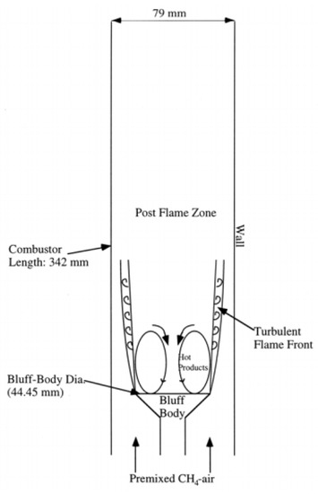
Figure 1.
A schematic diagram of bluff-body stabilised lean premixed combustor [36,37].

Table 1.
Combustor characteristics [36,37].
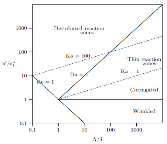
Figure 2.
The premixed combustion regime diagram [7].
These flames have been previously studied using the RANS partially premixed model [38] and LES flamelet [39]. The RANS study applied a steady-state partially premixed model with a single-step mechanism under adiabatic conditions. The PDF of the progress variable was modelled using a presumed shape with a beta function. The flame front position was determined by solving a transport equation for the mean reaction progress variable plus the mean mixture fraction and its variance. The turbulent flame speed in the premixed model was closed by Zimont turbulent flame speed closure. This model assumes that the combustion front consumes fuel at a turbulent flame speed [40]. In the LES study, Favre-filtered transport equations were solved. The sub-filter scalar term was modelled using the gradient-assumption with the turbulent Schmidt number, with a constant of 0.7. The sub-grid-scale viscosity was obtained from the standard Smagorinsky model. The turbulent flame speed was modelled by Zimont turbulent flame speed closure [40]. On the other hand, the contribution of CMC for premixed combustion would be predicting species with slow time scales, including the effects of turbulence on the chemical structure with complex chemical kinetics [19,20]. The proposed model for the conditional scalar dissipation rate term in the CMC transport equation is based on a mathematical approach and has no preassumptions [21].
5. Computational Approach and Parameters
The original version of the research code was designed for non-premixed flames with two separate streams [41], fuel and oxidiser, with their mixing being described by solving a transport equation for Favre averaged mixture fraction, which is a passive scalar. The code was further developed to include turbulent premixed flames [19,20] with more than two streams along with appropriate transport equations to track the fluids emerging from these various streams. The transport equations for the Favre averaged progress variable and its variance were also included in addition to closure for the mean reaction rate.
The partial differential equation for the stationary CMC transport equation was discretised over a physical space control volume into an algebraic equation by the finite volume method. The power-law scheme was used to discretise the physical and ζ space derivatives in the CMC equation. A SIMPLER approach [42] was used to couple the velocity and pressure fields inside the computational domain. These discretised equations were solved to obtain the conditional mean quantities using an iterative algorithm with under-relaxation factors, as shown in Table 2. The CMC transport equation was solved in space on the CMC physical grid by the CMC solver. The Favre-averaged mass, momentum, turbulence, enthalpy progress variable, progress variable variance, and the mixture fraction transport equations were solved on the RANS physical domain and passed to the CMC solver. The exchange process was iterated until convergence criteria were met. These convergence criteria were set to be 5 × 10⁻⁵ for fluid dynamics and CMC. The mean flow and turbulence quantities obtained from the fluid dynamics solver were passed to the CMC solver.
Table 2.
Under-relaxation factors.
The physical computational domain covered 79 342 mm in r and x directions with 180 × 513 cells in both directions. Based on the CMC assumption, the conditional averages changed gradually in the physical space. Thus, two cells in each direction of the physical domain were joined to assemble the physical grid for the CMC equations. The initial value of the progress variable variance entering the computational domain was zero. The bluff-body and combustion chamber walls were considered no-slip walls, and heat transfer from the walls was considered. The conditional mean reaction rate term was closed using a first-order CMC closure, and the GRI-3.0 [43] chemical mechanism was used to represent the chemical kinetics of the methane–air mixture. The initial and boundary conditions for the CMC equations in the ζ space were prescribed using planar unstrained laminar flame computation obtained from the Premix code of Chemkin [44]. A presumed shape with a beta model was used for the PDF of the progress variable. From the converged solution, the various mean quantities required for comparison with experimental measurements were obtained using Equation (10). Further details on the computational tool used in this study can be found in [19,20,41]. The computational sequence in the RANS-CMC framework is shown in Figure 3.
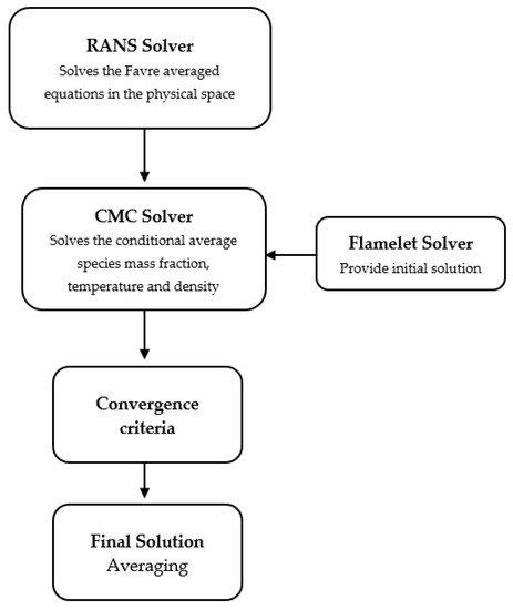
Figure 3.
The computational sequence in the RANS-CMC program [19,20].
6. Results and Discussion
The physical computational grid was specified to be non-uniform near the inlet and the bluff-body recirculation zone. The CMC grid consisted of 500 non-uniform cells in ζ space. As the conditional averages oscillated slowly in the physical space, the CMC physical space was constructed by combining two RANS grid cells. The conditional mean mass fraction Qα was obtained by solving the CMC equation, Equation (7), without eQα. The typical variation of conditional mean mass fractions for some selected species is shown in Figure 4. The results are shown for c = 0.586 at axial locations, x/D = 1.5. The values of and OH mass fractions were multiplied by 40 and 20 for plotting purposes, and the results were compared to the unstrained laminar methane–air premixed flame with φ = 0.58. The laminar calculations were obtained using the PREMIX code [44] and the GRI-mechanism.
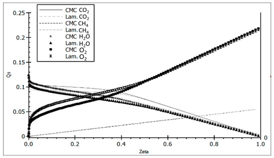
Figure 4.
Variation of the conditional mean mass fraction with ζ for major species at c = 0. 586 and x/D = 1.5.
The radial variations of the computed normalised mean axial velocity, temperature, and mole fractions of major species were compared to the experimental measurements at different axial locations in the flame, as shown in Figure 5, Figure 6, Figure 7, Figure 8 and Figure 9. The values were normalised using the axial inlet velocity. The solid lines represent the CMC calculations, and the symbols represent the experimental measurements [36,37]. The standard radial profiles of these scalars were satisfactory and acceptable at all axial locations in the flame. The normalised mean axial velocity was over-predicted in the upstream region close to the bluff-body circulation zone. These discrepancies can be attributed to the strong inhomogeneous turbulence near the burner exit. The comparison gradually improved far from the recirculation zone, where the turbulence intensity levels were low.
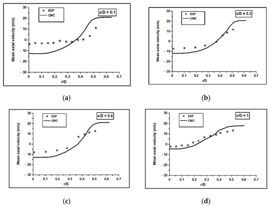
Figure 5.
The computed normalised mean velocity was compared to the experimental measurements at axial locations: (a) x/D = 0.1, (b) 0.3, (c) 0.6, and (d) 1 [36,37].
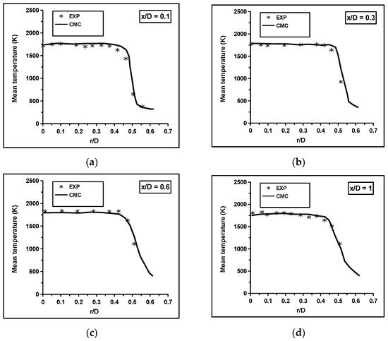
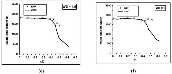
Figure 6.
The computed mean temperature was compared to the experimental measurements: (a) x/D = 0.1, (b) 0.3, (c) 0.6, (d) 1, (e) 1.5, and (f) 2 [36,37].
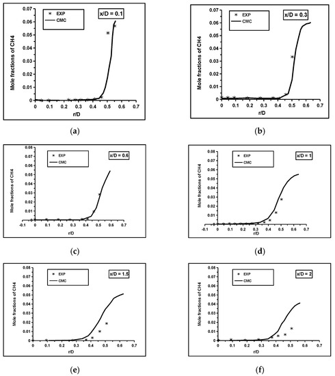
Figure 7.
The computed mean mole fractions of were compared to the experimental measurements: (a) x/D = 0.1, (b) 0.3, (c) 0.6, (d) 1, (e) 1.5, and (f) 2 [36,37].
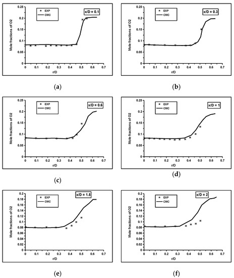
Figure 8.
The computed mean mole fractions of were compared to the experimental measurements: (a) x/D = 0.1, (b) 0.3, (c) 0.6, (d) 1, (e) 1.5, and (f) 2 [36,37].
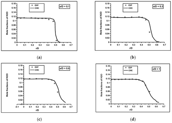
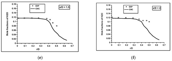
Figure 9.
The computed mean mole fractions of were compared to the experimental measurements: (a) x/D = 0.1, (b) 0.3, (c) 0.6, (d) 1, (e) 1.5, and (f) 2 [36,37].
Additionally, the differential diffusion effects were significant near the central and recirculation regions. Adding the differential diffusion terms to the CMC transport equation may improve the velocity profiles upstream. The peak temperature at the centre line was captured reasonably by the RANS-CMC framework, as shown in Figure 6. In the transverse direction, the agreement between the measured and computed mean values was acceptable inside the recirculation zone region at x/D < 1.0. Beyond this region, a steep temperature gradient was observed near the combustor wall at radial locations greater than 0.4. There was a comparable level of agreement for the major reactants and products profiles at all axial locations in the flame, as shown in Figure 7, Figure 8 and Figure 9. The CMC predicts reasonably the mean values at upstream locations x/D < 1.0. Outside this region, the mean values of the and were over-predicted at radial locations greater than 0.4, while the mean values of and were under-predicted. The discrepancies at downstream locations were possibly because of the model, and hence, a future study to address the sensitivity of the computations to different turbulence models are required to clarify these issues.
7. Summary and Conclusions
The implementation of the conditional moment closure (CMC) method to turbulent premixed combustion is still under research. In the method, the transport equations are derived without any explicit assumptions about how turbulent vortices affect the flame front structure. Therefore, finite-rate chemistry is expected to be well captured. Unlike other methods, this feature enables the CMC to predict chemically slow species, such as nitrogen oxides, with realistic computational costs. While this method has recently been amended and validated to turbulent premixed combustion with some encouraging outcomes, its sub-model precision significantly influences the method’s strength. Among the critical sub-models is the conditional scalar dissipation rate, representing the mixing at a small scale. This term describes the local micromixing of the relevant scalar. It signifies the dissipation rate of progress variable variance, which is predominantly affected by the coupling of turbulence, diffusion, and chemical reaction. Hence, this work aimed to implement an alternative model [21] for this term in the RANS-CMC framework and to use the method to compute lean premixed bluff-body stabilised turbulent flame. The PDF of the progress variable was modelled using a presumed shape with a beta function. The conditional mean reaction rate, , for species α in Equation (7) was closed using a first-order CMC closure [9], and the combustion kinetics were represented using the GRI-3.0 chemical kinetics mechanism for methane–air combustion. The standard k-ε represents the turbulence. Despite some discrepancies, especially within the recirculation zone where the turbulence intensity was very high, the RANS-CMC framework captured the general trend of premixed turbulent flame near blow-off conditions in reasonable agreement with experimental measurements. Additional approvement may be achieved by including the differential term in the CMC transport equation.
Author Contributions
Formal analysis, S.A.; funding acquisition, S.A.; investigation, S.A.; methodology, S.A.; project administration, S.A.; resources, M.F.M.Y.; software, S.A.; validation, S.A.; visualisation, S.A.; writing—original draft, S.A.; writing—review and editing, S.A. and M.F.M.Y. All authors have read and agreed to the published version of the manuscript.
Funding
This research received no external funding.
Institutional Review Board Statement
Not applicable.
Informed Consent Statement
Not applicable.
Data Availability Statement
The experimental data presented in this study is available from [36,37].
Conflicts of Interest
The authors declare no conflict of interest.
References
- Swaminathan, N.; Bray, K.N. Turbulent Premixed Flames; Cambridge University Press: Cambridge, UK, 2011; Available online: https://www.cambridge.org/core/books/turbulent-premixed-flames/FD00E0314B0872947BCD3661F63EC203 (accessed on 29 March 2021).
- Dowlin, A.P. The Challenges of Lean Premixed Combustion. In Proceedings of the International Gas Turbine Congress, Tokyo, Japan, 2–7 November 2003. [Google Scholar]
- Brewster, B.S.; Cannon, S.M.; Farmer, J.R.; Meng, F. Modelling of Lean Premixed Combustion in Stationary Gas Turbines. Prog. Energy Combust. Sci. 1999, 4, 353–385. [Google Scholar] [CrossRef]
- Correa, S.M. A review of NOx formation Under Gas Turbine Combustion Conditions. Combust. Sci. Technol. 1993, 87, 329–362. [Google Scholar] [CrossRef]
- Driscoll, J.F. Turbulent Premixed Combustion: Flamelet Structure and its Effect on Turbulent Burning Velocities. Prog. Energy Combust. Sci. 2008, 34, 91–134. [Google Scholar] [CrossRef]
- Huang, Y.; Yang, V. Dynamics and Stability of Lean-Premixed Swirl-stabilized Combustion. Prog. Energy Combust. Sci. 2009, 35, 293–364. [Google Scholar] [CrossRef]
- Echekki, T.; Mastorakos, E. Turbulent Combustion Modelling Advances, New Trends and Perspectives; Springer: Berlin/Heidelberg, Germany, 2011. [Google Scholar]
- Shimada, Y.; Thornber, B.; Drikakis, D. High-order Implicit Large Eddy Simulation of gaseous fuel injection and mixing of a bluff body burner. Comput. Fluids 2011, 44, 229–237. [Google Scholar] [CrossRef]
- Klimenko, A.Y.; Bilger, R.W. Conditional Moment Closure for Turbulent Combustion. Prog. Energy Combust. Sci. 1999, 25, 595–687. [Google Scholar] [CrossRef]
- Rogersson, J.W. Measurements and Modelling of a Bagasse-Fired Boiler. Ph.D. Thesis, The University of Sydney, Sydney, Australia, 2006. [Google Scholar]
- Kim, S.H.; Huh, K.Y.; Tao, L. Application of the elliptic Conditional Moment Closure model to a two-dimensional non-premixed methanol bluff body flame. Combust. Flame 1999, 120, 75–90. [Google Scholar] [CrossRef]
- Sreedhara, S.; Huh, K.Y. Modelling of turbulent two-dimensional non-premixed Methane-Hydrogen flame over a bluff body using first and second-order elliptic Conditional Moment Closure. Combust. Flame 2005, 143, 119–134. [Google Scholar] [CrossRef]
- Kim, S.; Mastorakos, E. Simulations of turbulent lifted jet flames with two-dimensional conditional Moment Closure. Proc. Combust. Inst. 2005, 30, 911–918. [Google Scholar] [CrossRef]
- Wright, Y.M.; De Paola, G.; Boulouchos, K.; Mastorakos, E. Simulations of spray autoignition and flame establishment with two-dimensional CMC. Combust. Flame 2005, 143, 402–419. [Google Scholar] [CrossRef]
- Zhang, H.; Giusti, A.; Mastorakos, E. LES/CMC Modelling of Ignition and Flame Propagation in a Non-premixed Methane Jet. Proc. Combust. Instit. 2018, 37, 2125–2132. [Google Scholar] [CrossRef]
- Sitte, M.P.; Mastorakos, E. Modelling of spray flames with Doubly Conditional Moment Closure. Flow Turb. Combust. 2017, 99, 933–954. [Google Scholar] [CrossRef] [PubMed]
- Zhang, H.; Mastorakos, E. LES/CMC Modelling of a Gas Turbine Model Combustor with Quick Fuel Mixing. Flow Turb. Combust. 2018, 102, 909–930. [Google Scholar] [CrossRef]
- Yunardi, Y.; Woolley, R.M.; Fairweather, M. Conditional Moment Closure prediction of soot formation in turbulent non-premixed ethylene flames. Combust. Flame 2008, 152, 360–376. [Google Scholar] [CrossRef]
- Amzin, S.; Swaminathan, N.; Rogerson, J.W.; Kent, J.H. Conditional Moment Closure for Turbulent Premixed Flames. Combust. Sci. Technol. 2012, 184, 1–25. [Google Scholar] [CrossRef]
- Amzin, S.; Swaminathan, N. Conditional Moment Closure for Turbulent Lean Premixed Flames. Combust. Theory Model. 2013, 17, 1125–1153. [Google Scholar] [CrossRef]
- Amzin, S.; Domagała, M. Modelling of Conditional Scalar Dissipation Rate in Turbulent Premixed Combustion. Computation 2021, 9, 26. [Google Scholar] [CrossRef]
- Farrace, D.; Chung, K.; Bolla, M.; Wright, Y.M.; Boulouchos, K.; Mastorakos, E. A LES-CMC formulation for premixed flames including differential diffusion. Combust. Theory Model. 2017, 22, 411–431. [Google Scholar] [CrossRef]
- Farrace, D.; Chung, K.; Pandurangi, S.S.; Wright, Y.M.; Boulouchos, K.; Swaminathan, N. Unstructured LES-CMC modelling of turbulent premixed bluff body flames close to blow-off. Proc. Combust. Instit. 2016, 36, 1977–1985. [Google Scholar] [CrossRef]
- Chen, Y.C.; Peters, N.; Schneemann, G.A.; Wruck, N.; Renz, U.; Mansour, M.S. The detailed flame structure of highly stretched turbulent premixed methane-air flames. Combust. Flame 1996, 107, 223–224. [Google Scholar] [CrossRef]
- Dunn, M.J.; Masri, A.R.; Bilger, R.W. A new piloted premixed jet burner to study strong finite-rate chemistry effects. Combust. Flame 2007, 151, 46–60. [Google Scholar] [CrossRef]
- Kolla, H.; Rogerson, J.W.; Swaminathan, N. Scalar Dissipation Rate Modelling and its Validation. Combust. Sci. Tech. 2009, 181, 518–535. [Google Scholar] [CrossRef]
- Veynante, D.; Vervisch, L. Turbulent Combustion Modelling. Prog. Energy Combust. Sci. 2002, 28, 193–266. [Google Scholar] [CrossRef]
- Poinsot, T.; Veyante, D. Theoretical and Numerical Combustion, 2nd ed.; Westview Press: Philadelphia, PA, USA, 2005. [Google Scholar]
- Swaminathan, N.; Bilger, R.W. Analysis of Conditional Moment Closure for Turbulent Premixed Flames. Combust. Theory Model. 2001, 5, 241–260. [Google Scholar] [CrossRef]
- Colucci, P.J.; Jaberi, F.A.; Givi, P.; Pope, S.B. Filtered Density Function for Large Eddy Simulation of Turbulent Reacting Flows. Phys. Fluids. 1998, 10, 499–515. [Google Scholar] [CrossRef]
- Pope, S.B. An Explanation of the Turbulent Round Jet/Plane Jet Anomaly. AIAA J. 1980, 16, 279–281. [Google Scholar] [CrossRef]
- Tikhonov, A.N.; Goncharsky, A. Numerical Method for the Solution of Ill-Posed Problems; Kluwer Academic: Moscow, Russia, 1990. [Google Scholar]
- Bushe, W.K.; Steiner, H. Conditional Moment Closure for Large Eddy Simulation of Non-Premixed Turbulent Reacting. Flows Phys. Fluids 1999, 11, 1896–1906. [Google Scholar] [CrossRef]
- Steiner, H.; Bushe, W.K. Large-eddy Simulation of a Turbulent Reacting Jet with Conditional Source Term Estimation. Phys. Fluids 2001, 13, 754–769. [Google Scholar] [CrossRef]
- Hestenes, M.R.; Stiefel, E. Methods of Conjugate Gradients for Solving Linear Systems. J. Res. Nat. Bur. Stand. 1952, 49, 409–435. [Google Scholar] [CrossRef]
- Nandula, S.; Pitz, R.; Barlow, R.; Fiechtner, G. Rayleigh/Raman/LIF measurements in a turbulent lean premixed combustor. In Proceedings of the 34th Aerospace Sciences Meeting and Exhibit, Reno, NV, USA, 15–18 January 1996. [Google Scholar]
- Nandula., S. Lean Premixed Flame Structure in Intense Turbulence: Rayleigh/Raman/LIF Measurements and Modelling. Ph.D. Thesis, Faculty of the Graduate School, Vanderbilt University, Nashville, TN, USA, 2003. Available online: https://ui.adsabs.harvard.edu/abs/2003PhDT........33N/abstract (accessed on 29 March 2021).
- Andreini, A.; Bianchini, C.; Innocenti, A. Large Eddy Simulation of a Bluff Body Stabilized Lean Premixed Flame. J. Combust. 2014, 2014, 710254. [Google Scholar] [CrossRef]
- Sudarma, A.F.; Al-Witry, A.; Morsy, M.H. RANS Numerical Simulation of Lean Premixed Bluff Body Stabilized Combustor: Comparison of Turbulence Models. J. Thermal Eng. 2017, 3, 1561–1573. [Google Scholar] [CrossRef]
- Zimont, V. Theory of Turbulent Combustion of a Homogeneous Fuel Mixture at High Reynolds Numbers. Combust. Explos. Shock Waves 1979, 15, 305–311. [Google Scholar] [CrossRef]
- Rogerson, J.W.; Kent, J.H.; Bilger, R.W. Conditional moment closure in a bagasse-fired boiler. Proc. Combust. Inst. 2007, 31, 2805–2811. [Google Scholar] [CrossRef]
- Patankar, S.V. Numerical Heat Transfer and Fluid Flow; Hemisphere: Washington, DC, USA, 1980. [Google Scholar]
- Smith, G.P.; Golden, D.M.; Frenklach, M.; Moriarty, N.W.; Eiteneer, B.; Goldenberg, M.; Thomas Bowman, C.; Hanson, R.K.; Song, S.; Gardiner, W.C., Jr.; et al. GRI-Mech 3.0; The Gas Research Institute: Des Plaines, IL, USA, 2011; Available online: http://www.me.berkeley.edu/grimech (accessed on 29 March 2021).
- Kee, R.J.; Grcar, J.F.; Smooke, M.D.; Miller, J.A. A Fortran Program. For Modelling Steady Laminar One-Dimensional Premixed Flames; Report SAND85-8240; Sandia National Laboratories: Livermore, CA, USA, 1985. [Google Scholar]


Publisher’s Note: MDPI stays neutral with regard to jurisdictional claims in published maps and institutional affiliations. |
© 2021 by the authors. Licensee MDPI, Basel, Switzerland. This article is an open access article distributed under the terms and conditions of the Creative Commons Attribution (CC BY) license (https://creativecommons.org/licenses/by/4.0/).