
Artificial Intelligence-Based Optimization of a Bimorph-Segmented Tapered Piezoelectric MEMS Energy Harvester for Multimode Operation


Abstract
:1. Introduction
2. Materials and Methods
2.1. Theoretical Model
2.1.1. Estimation of Natural Frequency
2.1.2. Estimation of General Power
2.2. Numerical Model
3. AI-Assisted Software Solution
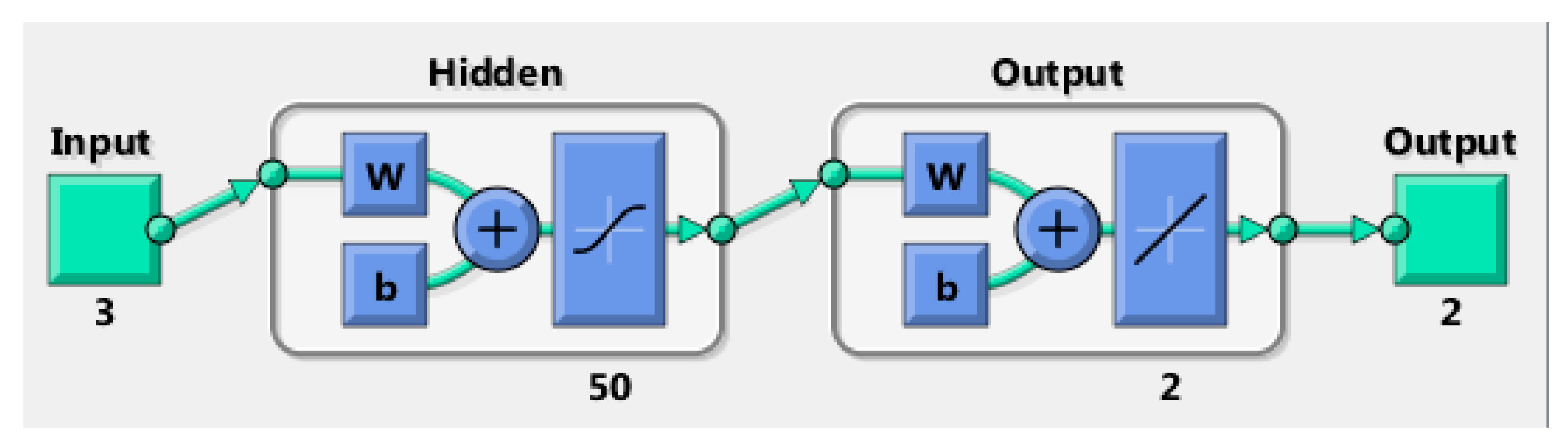
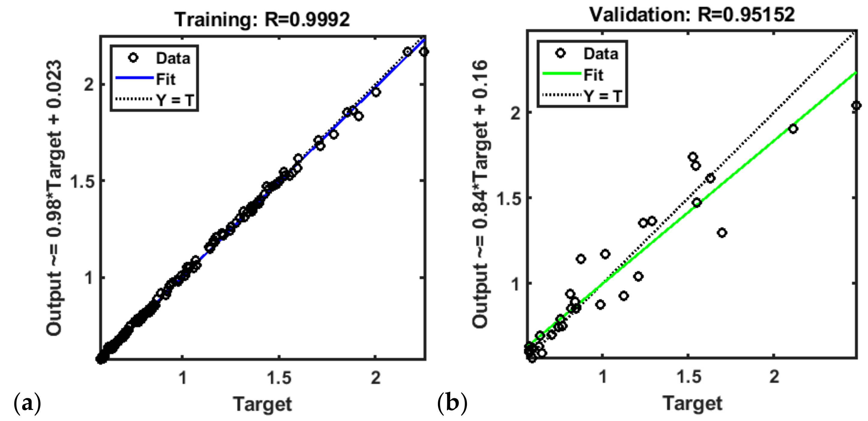
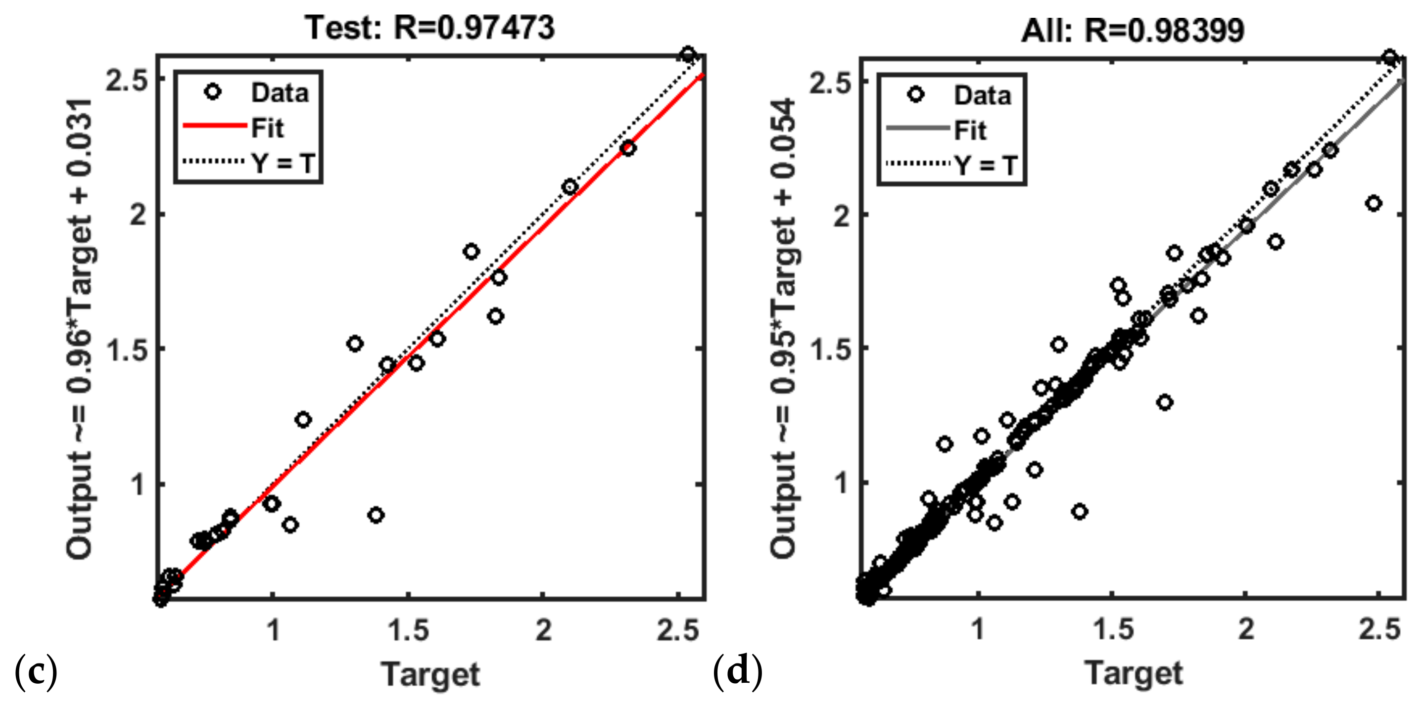
3.1. ANN Capable of Predicting Frequency and Power of the First Resonant Mode
3.2. Optimization: Goal Attainment Method and Genetic Algorithm
4. Results
5. Conclusions
Author Contributions
Funding
Data Availability Statement
Acknowledgments
Conflicts of Interest
References
- Roundy, S.; Wright, P.K. A piezoelectric vibration based generator for wireless electronics. Smart Mater. Struct. 2004, 13, 1131. [Google Scholar] [CrossRef] [Green Version]
- Sil, I.; Biswas, K. Investigation of Design Parameters in MEMS Based Piezoelectric Vibration Energy Harvester. In Proceedings of the International Conference on 2018 IEEE Electron Device Kolkata Conference (EDKCON), Kolkata, India, 24–25 November 2018; pp. 64–69. [Google Scholar] [CrossRef]
- Baker, J.L.; Roundy, S.; Wright, P. Alternative geometries for increasing power density in vibration energy scavenging for wireless sensor networks. In Proceedings of the 3rd International Energy Conversion Engineering Conference, San Francisco, CA, USA, 18 August 2005; p. 5617. [Google Scholar] [CrossRef] [Green Version]
- Pertin, O.; Shrivas, P.; Guha, K.; Rao, K.S.; Iannacci, J. New and efficient design of multimode piezoelectric vibration energy harvester for MEMS application. Microsyst. Technol. 2021, 27, 3523–3531. [Google Scholar] [CrossRef]
- Almeida, B.V.D.; Pavanello, R. Topology optimization of the thickness profile of bimorph piezoelectric energy harvesting devices. J. Appl. Comput. Mech. 2019, 5, 113–127. [Google Scholar] [CrossRef]
- Erturk, A.; Tarazaga, P.A.; Farmer, J.R.; Inman, D.J. Effect of strain nodes and electrode configuration on piezoelectric energy harvesting from cantilevered beams. J. Vib. Acoust. Trans. 2009, 131, 01101011. [Google Scholar] [CrossRef] [Green Version]
- Krishnasamy, M.; Lenka, T.R. Distributed parameter model for assorted piezoelectric harvester to prevent charge cancellation. IEEE Sens. Lett. 2017, 1, 1–4. [Google Scholar] [CrossRef]
- Ferrari, M.; Ferrari, V.; Guizzetti, M.; Marioli, D.; Taroni, A. Piezoelectric multifrequency energy converter for power harvesting in autonomous microsystems. Sens. Actuators A Phys. 2008, 142, 329–335. [Google Scholar] [CrossRef]
- Qi, S.; Shuttleworth, R.; Oyadiji, S.O.; Wright, J. Design of a multiresonant beam for broadband piezoelectric energy harvesting. Smart Mater. Struct. 2010, 19, 094009. [Google Scholar] [CrossRef]
- Mažeika, D.; Čeponis, A.; Yang, Y. Multifrequency piezoelectric energy harvester based on polygon-shaped cantilever array. Shock. Vib. 2018, 2018, 11. [Google Scholar] [CrossRef] [Green Version]
- Janusas, G.; Milasauskaite, I.; Ostasevicius, V.; Dauksevicius, R. Efficiency improvement of energy harvester at higher frequencies. J. Vibroeng. 2014, 16, 1326–1333. [Google Scholar]
- Jabbari, M.; Ghayour, M.; Mirdamadi, H.R. Increasing the performance of energy harvesting in vibration mode shapes. Adv. Comput. Des. 2016, 1, 155–173. [Google Scholar] [CrossRef]
- Ostasevicius, V.; Gaidys, R.; Dauksevicius, R. Numerical analysis of dynamic effects of a nonlinear vibro-impact process for enhancing the reliability of contact-type MEMS devices. Sensors 2009, 9, 10201–10216. [Google Scholar] [CrossRef] [Green Version]
- Ghatkesar, M.K.; Barwich, V.; Braun, T.; Ramseyer, J.P.; Gerber, C.; Hegner, M.; Despont, M. Higher modes of vibration increase mass sensitivity in nanomechanical microcantilevers. Nanotechnology 2007, 18, 445502. [Google Scholar] [CrossRef] [Green Version]
- Fu, M.C. Optimization via simulation: A review. Ann. Oper. Res. 1994, 53, 199–247. [Google Scholar] [CrossRef]
- Park, J.C.; Lee, D.H.; Park, J.Y.; Chang, Y.S.; Lee, Y.P. High performance piezoelectric MEMS energy harvester based on D33 mode of PZT thin film on buffer-layer with PBTIO3 inter-layer. In Proceedings of the TRANSDUCERS 2009–2009 International Solid-State Sensors, Actuators and Microsystems Conference, Denver, CO, USA, 21–25 June 2009; IEEE: Piscataway, NJ, USA, 2009; pp. 517–520. [Google Scholar] [CrossRef]
- Bagheri, S.; Wu, N.; Filizadeh, S. Simulation-based optimization of a piezoelectric energy harvester using artificial neural networks and genetic algorithm. In Proceedings of the 2019 IEEE 28th International Symposium on Industrial Electronics (ISIE), Vancouver, BC, Canada, 12–14 June 2019; IEEE: Piscataway, NJ, USA, 2019; pp. 1435–1440. [Google Scholar] [CrossRef]
- Mohammadi, S.; Cheraghi, K.; Khodayari, A. Piezoelectric vibration energy harvesting using strain energy method. Eng. Res. Express 2019, 1, 015033. [Google Scholar] [CrossRef]
- Keshmiri, A.; Bagheri, S.; Wu, N. Simulation-Based Optimization of a Non-Uniform Piezoelectric Energy Harvester with Stack Boundary. Int. J. Mech. Mater. Eng. 2019, 13, 500–505. [Google Scholar]
- Nabavi, S.; Zhang, L. Design and optimization of wideband multimode piezoelectric MEMS vibration energy harvesters. Multidiscip. Digit. Publ. Inst. Proc. 2017, 1, 586. [Google Scholar] [CrossRef] [Green Version]
- Singh, K.B.; Bedekar, V.; Taheri, S.; Priya, S. Piezoelectric vibration energy harvesting system with an adaptive frequency tuning mechanism for intelligent tires. Mechatronics 2012, 22, 970–988. [Google Scholar] [CrossRef]
- Nawir, N.A.A.; Basari, A.A.; Saat, M.S.M.; Yan, N.X.; Hashimoto, S. A review on piezoelectric energy harvester and its power conditioning circuit. ARPN J. 2018, 13, 2993–3006. [Google Scholar]
- Yang, Z.; Zhou, S.; Zu, J.; Inman, D. High-performance piezoelectric energy harvesters and their applications. Joule 2018, 2, 642–697. [Google Scholar] [CrossRef] [Green Version]
- Kuo, Y.C.; Chien, J.T.; Shih, W.T.; Chen, C.T.; Lin, S.C.; Wu, W.J. The fatigue behavior study of micro piezoelectric energy harvester under different working temperature. In Active and Passive Smart Structures and Integrated Systems XII; International Society for Optics and Photonics: Bellingham, WA, USA, 2019; Volume 10967. [Google Scholar] [CrossRef]
- Chen, C.T.; Fu, Y.H.; Tang, W.H.; Lin, S.C.; Wu, W.J. The output power improvement and durability with different shape of MEMS piezoelectric energy harvester. In Smart Structures and NDE for Industry 4.0; International Society for Optics and Photonics: Bellingham, WA, USA, 2018; Volume 10602, p. 106020N. [Google Scholar] [CrossRef]
- Farhangdoust, S.; Georgeson, G.; Ihn, J.B.; Chang, F.K. Kirigami auxetic structure for high efficiency power harvesting in self-powered and wireless structural health monitoring systems. Smart Mater. Struct. 2020, 30, 015037. [Google Scholar] [CrossRef]
- Wu, H.; Tang, L.; Yang, Y.; Soh, C.K. A novel two-degrees-of-freedom piezoelectric energy harvester. J. Intell. Mater. Syst. Struct. 2013, 24, 357–368. [Google Scholar] [CrossRef]
- Nabavi, S.; Zhang, L. Design and optimization of a low-resonant-frequency piezoelectric MEMS energy harvester based on artificial intelligence. Multidiscip. Digit. Publ. Inst. Proc. 2018, 2, 930. [Google Scholar] [CrossRef] [Green Version]
- Sunithamani, S.; Lakshmi, P.; Flora, E.E. PZT length optimization of MEMS piezoelectric energy harvester with a non-traditional cross section: Simulation study. Microsyst. Technol. 2014, 20, 2165–2171. [Google Scholar] [CrossRef]
- Erturk, A.; Inman, D.J. An experimentally validated bimorph cantilever model for piezoelectric energy harvesting from base excitations. Smart Mater. Struct. 2009, 18, 025009. [Google Scholar] [CrossRef]
- Mitchell, M. An Introduction to Genetic Algorithms; MIT Press: Cambridge, MA, USA, 1998; ISBN 0262631857. [Google Scholar]
- Nabavi, S.; Zhang, L. Nonlinear multi-mode wideband piezoelectric mems vibration energy harvester. IEEE Sens. J. 2019, 19, 4837–4848. [Google Scholar] [CrossRef]
- Li, X.; Upadrashta, D.; Yu, K.; Yang, Y. Analytical modeling and validation of multi-mode piezoelectric energy harvester. Mech. Syst. Signal Process. 2019, 124, 613–631. [Google Scholar] [CrossRef]
- Wang, H.; Tang, L.; Shan, X.; Xie, T.; Yang, Y. Modeling and comparison of cantilevered piezoelectric energy harvester with segmented and continuous electrode configurations. In Active and Passive Smart Structures and Integrated Systems 2013; International Society for Optics and Photonics: Bellingham, WA, USA, 2013; Volume 8688, p. 86882B. [Google Scholar] [CrossRef]
- Nabavi, S.; Zhang, L. Design and optimization of piezoelectric MEMS vibration energy harvesters based on genetic algorithm. IEEE Sens. J. 2017, 17, 7372–7382. [Google Scholar] [CrossRef]
- Nabavi, S.; Zhang, L. Frequency tuning and efficiency improvement of piezoelectric MEMS vibration energy harvesters. J. Microelectromech. Syst. 2018, 28, 77–87. [Google Scholar] [CrossRef]
- Goldschmidtboeing, F.; Woias, P. Characterization of different beam shapes for piezoelectric energy harvesting. J. Micromech. Microeng. 2008, 18, 104013. [Google Scholar] [CrossRef]
- Jackson, N.; O’Keeffe, R.; Waldron, F.; O’Neill, M.; Mathewson, A. Evaluation of low-acceleration MEMS piezoelectric energy harvesting devices. Microsyst. Technol. 2014, 20, 671–680. [Google Scholar] [CrossRef]
- Ramírez, J.M.; Gatti, C.D.; Machado, S.P.; Febbo, M. A multi-modal energy harvesting device for low-frequency vibrations. Extrem. Mech. Lett. 2018, 22, 1–7. [Google Scholar] [CrossRef]
- Zergoune, Z.; Kacem, N.; Bouhaddi, N. On the energy localization in weakly coupled oscillators for electromagnetic vibration energy harvesting. Smart Mater. Struct. 2019, 28, 07LT02. [Google Scholar] [CrossRef] [Green Version]
- Gatti, C.; Ramirez, J.; Febbo, M.; Machado, S. Multimodal piezoelectric device for energy harvesting from engine vibration. J. Mech. Mater. Struct. 2018, 13, 17–34. [Google Scholar] [CrossRef]
- Aouali, K.; Kacem, N.; Bouhaddi, N.; Mrabet, E.; Haddar, M. Efficient broadband vibration energy harvesting based on tuned non-linearity and energy localization. Smart Mater. Struct. 2020, 29, 10LT01. [Google Scholar] [CrossRef]
- Jakšić, O. ANN Assisted Optimization of a Multimode Linearly Tapered Bimorph PYT-5 Cantilever Beam for Low Frequency Energy Harvesting; Version 1; Elsevier: Amsterdam, The Netherlands, 2021. [Google Scholar] [CrossRef]


| Parameter | Description | Value |
|---|---|---|
| L | Length of beam | 80–100 mm |
| Beam Width at fixed end (x = 0) | 2–3 mm | |
| Beam width at free end (x = L) | 20–30 mm | |
| Thickness of PZT | 0.5 mm | |
| Thickness of steel substrate | 1 mm | |
| Density of PZT | 7500 (kg/) | |
| Density of steel | 7850 (kg/) | |
| Young Modulus of PZT | 64 (GPa) | |
| Young Modulus of steel | 200 (GPa) | |
| Piezoelectric constant | −16.6 (C/ | |
| Permittivity constant | 25.55 (nF/) | |
| Tip Mass | 12.56–18.84 (mg) | |
| d | Separation between PZTs | 0.5 mm |
| Mode | Strain Node Position on the x-Axis = | ||
|---|---|---|---|
| 1st | 2nd | 3rd | |
| 1 | _ | _ | _ |
| 2 | 0.26 | _ | _ |
| 3 | 0.1468 | 0.490 | _ |
| 4 | 0.130 | 0.430 | 0.611 |
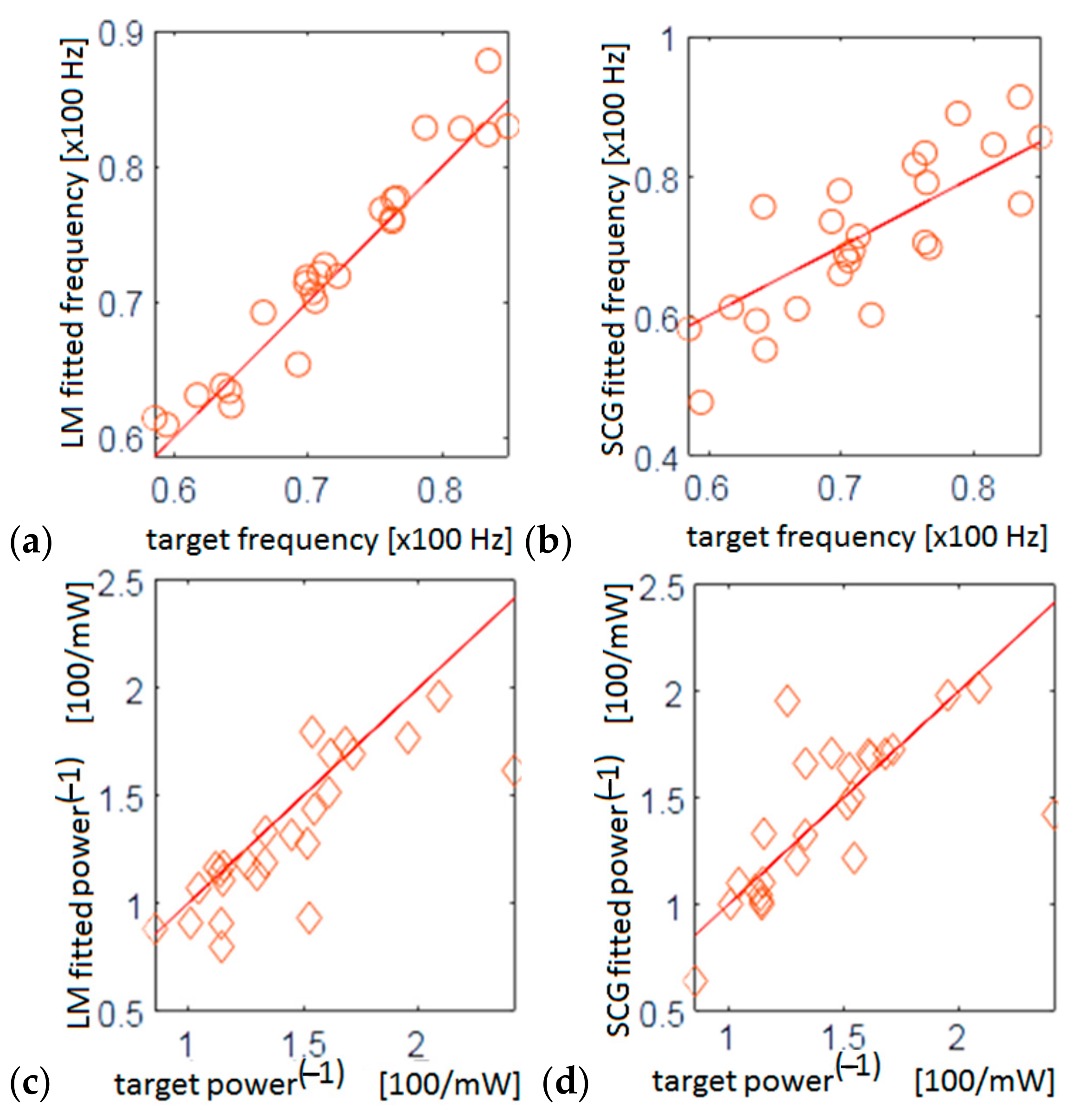
| LM | SCG | |
|---|---|---|
| Normalized frequency | 3.8398 × 10⁻⁴ | 0.0043 |
| Normalized reciprocal power | 0.0585 | 0.0774 |
| Triplet | ANN/ Optimization | Bounds or Starting Point | Scalar | |
|---|---|---|---|---|
| 1 | 117.98, 66.06, 0.7276 | SCG/GAM | [80 20 0.7] | 0.13 |
| 2 | 114.9, 72.69, 0.15 | LM/GA | [0.1;0.1;0], [1.5;1.5;1] | 0.1336 |
| 3 | 115.87, 73.73, 0.1983 | LM/GAM | [70 35 0.7] | 0.135 |
| 4 | 111.64, 39.88, 0.2525 | LM/GAM | [90 35 0.3] | 0.3935 |
| 5 | 121.3, 71.56, 0.7682 | SCG/GA | [0.1;0.1;0.1], [1.5;1.5;1] | 0.132 |
| 6 | 101.88, 19.45, 0.8636 | SCG/GAM | [70 35 0.7] | 0.7162 |
| Triplet | |||||||
|---|---|---|---|---|---|---|---|
| 1 | 117.98, 66.06, 0.7276 | 46.279 | 191.05 | 232.69 | 2.3735 | 338.77 | 2.9661 |
| 2 | 114.9, 72.69, 0.15 | 38.411 | 172.7 | 136.71 | 3.5471 | 312 | 0.63 |
| 3 | 115.87, 73.73, 0.1983 | 38.244 | 174.21 | 142.46 | 3.6312 | 308.9 | 1.209 |
| 4 | 111.64, 39.88, 0.2525 | 40.797 | 128.6 | 267.6 | 0.90212 | 331.7 | 0.94383 |
| 5 | 121.3, 71.56, 0.7682 | 44.3 | 205.56 | 211.6 | 2.7964 | 322.85 | 3.1552 |
| 6 | 101.88, 19.45, 0.8636 | 48.328 | 73.468 | 391.8 | 1278 | 607.74 | 7.95 × 10⁻⁵ |
| S.no | Triplet | Normalized Power (mW/g2) | ||
|---|---|---|---|---|
| T | Mode 1 | Mode 2 | Mode 3 | |
| 1 | 117.98, 66.06, 0.7276 | 764 | 9.494 | 11.864 |
| 2 | 114.9, 72.69, 0.15 | 690.8 | 14.188 | 2.52 |
| 3 | 115.87, 73.73, 0.1983 | 696.84 | 14.5248 | 4.836 |
| 4 | 111.64, 39.88, 0.2525 | 514.4 | 3.6 | 3.775 |
| 5 | 121.3, 71.56, 0.7682 | 822.24 | 11.1856 | 12.621 |
| 6 | 101.88, 19.45, 0.8636 | 293.872 | 5.112 | 0.00032 |
| Multi-Frequency Harvester | Acceleration (g) | Normalized Power (mW/g2) | ||
|---|---|---|---|---|
| Mode 1 | Mode 2 | Mode 3 | ||
| Array Harvester [8] | 1 | 0.089 | 0.057 | 0.057 |
| Optimized Nonlinear [32] | 0.05 | 0.008 | 0.244 | 0.056 |
| Nonlinear 3-DOF [33] | 0.2 | 46.739 | 0.568 | 1.538 |
| Segmented Electrode [34] | 1 | 5.800 | 0.121 | |
| Optimized, Tapered and Segmented [Our work] | 0.5 | 822.24 | 11.1856 | 12.621 |
Publisher’s Note: MDPI stays neutral with regard to jurisdictional claims in published maps and institutional affiliations. |
© 2021 by the authors. Licensee MDPI, Basel, Switzerland. This article is an open access article distributed under the terms and conditions of the Creative Commons Attribution (CC BY) license (https://creativecommons.org/licenses/by/4.0/).
Share and Cite
Pertin, O.; Guha, K.; Jakšić, O. Artificial Intelligence-Based Optimization of a Bimorph-Segmented Tapered Piezoelectric MEMS Energy Harvester for Multimode Operation. Computation 2021, 9, 84. https://doi.org/10.3390/computation9080084
Pertin O, Guha K, Jakšić O. Artificial Intelligence-Based Optimization of a Bimorph-Segmented Tapered Piezoelectric MEMS Energy Harvester for Multimode Operation. Computation. 2021; 9(8):84. https://doi.org/10.3390/computation9080084
Chicago/Turabian StylePertin, Osor, Koushik Guha, and Olga Jakšić. 2021. "Artificial Intelligence-Based Optimization of a Bimorph-Segmented Tapered Piezoelectric MEMS Energy Harvester for Multimode Operation" Computation 9, no. 8: 84. https://doi.org/10.3390/computation9080084
APA StylePertin, O., Guha, K., & Jakšić, O. (2021). Artificial Intelligence-Based Optimization of a Bimorph-Segmented Tapered Piezoelectric MEMS Energy Harvester for Multimode Operation. Computation, 9(8), 84. https://doi.org/10.3390/computation9080084