Abstract
In the pulp and paper industry, pulp testing is typically a labor-intensive process performed on hand-made laboratory sheets. Online quality control by automated image analysis and machine learning (ML) could provide a consistent, fast and cost-efficient alternative. In this study, four different supervised ML techniques—Lasso regression, support vector machine (SVM), feed-forward neural networks (FFNN), and recurrent neural networks (RNN)—were applied to fiber data obtained from fiber suspension micrographs analyzed by two separate image analysis software. With the built-in software of a commercial fiber analyzer optimized for speed, the maximum accuracy of 81% was achieved using the FFNN algorithm with Yeo–Johnson preprocessing. With an in-house algorithm adapted for ML by an extended set of particle attributes, a maximum accuracy of 96% was achieved with Lasso regression. A parameter capturing the average intensity of the particle in the micrograph, only available from the latter software, has a particularly strong predictive capability. The high accuracy and sensitivity of the ML results indicate that such a strategy could be very useful for quality control of fiber dispersions.
1. Introduction
The development of machine learning (ML) has accelerated, and its industrial applicability for, e.g., the pulp and paper industry, has increased dramatically during the last few years. These advancements, in combination with the possibility to automatically measure geometrical data from micrographs for large sets of particles, enable improved quality control, reduced global footprint and lowered manufacturing costs of materials comprising cellulose fibers [1,2].
Traditionally, pulp quality in the pulp and paper industry is assessed by manual preparation and testing of hand sheets. Although these laboratory methods are valuable, they are time consuming and cost ineffective. Furthermore, due to the time lag of such testing, it does not provide real-time quality control of production. This means that substandard production is observed and adjusted with substantial delay. Although laboratory testing of pulp will also be necessary in the future, there is a need for complementary, automated quality control systems which provide real-time pulp quality feedback. Online imaging systems for fiber distribution analysis, eventually combined with ML software, can be used to meet those requirements [1,3,4].
Pulp particle classes such as shives, fibers, vessel cells, and fine particles are established concepts in pulping and papermaking when discussing pulp quality. Indeed, size-based partitioning of pulp particles into classes is implemented in commercial optical fiber analyzers today. In this work, we set out to refine and automate pulp particle classification using ML techniques and thereby enhance the alignment between pulp particle classification of engineer users and analyzers while also supporting classification of a greater number of particle classes.
Image analysis is a technique used to extract valuable information from digital images. The process typically unfolds in several stages. It begins with the capture of high-quality digital images using a high-resolution camera, with subsequent image enhancement. The next step involves identifying and segmenting the subject of interest, such as fibers within digital images of pulp. The process concludes with the measurement of salient parameters of the specimen and interpretation of the resultant data [5].
As input to image analysis, digital images of cellulose fibers can be obtained by a variety of microscopy methods. These methods include scanning electron microscopy (SEM) and transmission electron microscopy (TEM) as well as microscopy based on optical light, X-rays, ultraviolet light (UV-vis), near-infrared light (NIR) and changes in polarized light (CPL) [3]. New advances in, e.g., computed tomography (CT) [5] have also enabled high-resolution three-dimensional images of fiber structures. The mechanical properties of the pulp are strongly affected by the complex microstructures of the fibers, which can be revealed with microscopy methods [6,7].
In this study, micrographs were obtained by optical light microscopy using fiber analysis equipment (L&W Fiber Tester plus, ABB). This equipment includes built-in image analysis software with five output parameters: fiber length, fiber width, fiber shape, area-based fibrillation and perimeter-based fibrillation [3]. These particle parameters provide pulp characterization in excellent detail to the human user. However, to exploit potentially untapped particle-level information that may be meaningful to ML algorithms, a complementary, in-house image analysis program was implemented with additional output parameters, e.g., light attenuation of the particles. ML algorithms were applied both with and without using the extra image parameters, thereby assessing whether the extra parameters could facilitate classification of different pulp particles.
ML, a subfield of artificial intelligence, is an important tool for automated analysis of big datasets. It can be seen as a collection of methods used to create algorithms which enable the computer to learn patterns from the input data [8]. The use of ML in the industry plays a major role in the advancement of the fourth industrial revolution ‘Industry 4.0’, which adopts such methods to increase efficiency in manufacturing and processing [9]. Advancements in ML have enabled a range of computational image analysis methods, which often surpass the human eye in a variety of fields [10]. With an automated characterization method, more precise and efficient quality control can be obtained. Combining ML with image analysis enables the use of online and offline measurements for improved, automated categorization of pulp and paper [1,3,11]. The potential cost reduction by implementing ML based on existing and future technologies in the paper and forest product industry is estimated to be 9.5% [12].
ML is often separated into supervised and unsupervised learning, where the former is currently more common [8]. The aim of supervised ML is to have the computer learn patterns from a labeled training set and use this to predict patterns for unlabeled data, whereas unsupervised learning considers unlabeled data. Therefore, supervised ML methods such as logistic regression, decision trees and linear model trees are often used to classify objects. Artificial neural networks (ANNs) are a type of deep learning methods which can be supervised or unsupervised. They mimic the biological nervous systems of the human brain, enabling models to process a large number of parameters and learn from experience [13]. Herein, we use different supervised MLs, including supervised ANNs, for pulp particle classification.
Even though ML combined with automated image analysis has the potential to reduce both cost and energy usage in the pulp and paper industry, this combination has not, to the best of our knowledge, been previously used to systematically classify cellulose fibers and debris in pulp, even though ML has recently been used for many other pulp and paper processing applications. Devi et al. described ways to utilize ML techniques for improving paper quality by optimizing process parameters [14], Nisi et al. applied multi-objective optimization techniques on pulp and paper processes [15], Jauhar et al. used neural network methods to improve the efficiency of Indian pulp and paper industries [16], and Narciso et al. wrote an review paper on ways to use ML tools to reduce energy consumption in industries [17]. Othen et al. described how to use ML techniques for predicting cardboard properties [18] and Parente et al. showed the ways in which Monte Carlo techniques can be used to pre-process data intended for ML-based “fault detection and diagnosis” models for pulping industries [19]. Talebjedi et al. used deep learning ML techniques to analyze the effect of different process parameters in TMP pulp mills [20] and to develop optimization strategies for energy saving in such facilities [21]. However, none of the aforementioned papers apply ML techniques directly on fiber data.
In this study, four different ML methods were assessed by comparing their ability to classify fibers and other pulp components. Pulp suspension micrographs were obtained using an optical fiber analyzer, and the micrographs were analyzed using the built-in software and an in-house image analysis software, which includes additional parameters such as the light attenuation of particles to uncover whether the extra parameters could further improve the accuracy of the classification. ML methods can be used improve the results obtained by optical fiber analysers, but do not eliminate the necessity of using such hardware.
2. Experimental Section
Thermomechanical pulp samples were extracted in Holmen Braviken pulp mill (Holmen, Stockholm, Sweden), where the raw material was a mix of 70% roundwood chips and 30% sawmill chips, both from Norway spruce (Picea abies). A chip refiner of type RGP68DD from Valmet was used and run at a specific energy of 1060 kWh/t (dry pulp). Pulp samples were extracted from the latency chest after the refiner, at a consistency of 4%, dewatered on a Büchner funnel with a 100-mesh wire, and the filtrate was recirculated once before freezing. The pulp samples were removed from the freezer one day before testing to defrost at room temperature, followed by hot disintegration according to ISO 5263-3:2023 [22].
The pulp samples were analyzed in a L&W Fiber Tester plus from ABB [23]. Fiber Tester follows relevant TAPPI/ISO standards, such as ISO-16065-2:2014 [24]. In accordance with recommendations, 100 L beakers of 0.100% consistency pulp suspension were used. The pulp was further diluted to 20 ppm in the analyzer. Inside the machine, the suspension was pumped through a narrow rectangular cross-section where grayscale images were captured using a digital camera with a stroboscope flash. The images were analyzed using built-in and in-house software (Section 3.1).
The built-in image analysis was set to capture all objects longer than 100 and thinner than 75 , and the instrument had a pixel resolution that enables detection of objects down to 6.6 . The setting with a minimum fiber length of 0.1 was in agreement with, e.g., TAPPI-standard 271 [25]. Each identified object was exported as a separate image, and the five measured parameters (contour length, width, shape factor, perimeter-based fibrillation, and area-based fibrillation) of each particle were saved in one data file. Particle contour length and width W were calculated from the measured particle area A and perimeter P. Fibers with approximately band-shaped geometry were assumed, so that
Shape factor S, which measures the straightness of the particle, was calculated as
where is the Euclidean distance between the two most distant points (endpoints) of the particle. Perimeter-based fibrillation and area-based fibrillation both correlated to the number of fibrils on the particle calculated from the light gray halo surrounding each fiber [26].
The Technical Association of the Pulp and Paper Industry (TAPPI) and the International Organization for Standardization (ISO) have defined standards for measuring many fiber properties. For instance, the measurement of average fiber length can be performed manually using TAPPI standards 232 (Fiber length of pulp by projection) [27] and 233 (Fiber length of pulp by classification) [28] or automatically using TAPPI 271 (Fiber length of pulp and paper by automated optical analyzer using polarized light) [25], ISO 16065-1 (Pulps—Determination of fiber length by automated optical analysis—Part 1: Polarized light method) [29] and ISO 16065-2 (Pulps – Determination of fiber length by automated optical analysis—Part 2: Unpolarized light method) [24]. It can be noted that many of the traditional standards for measuring fiber length, such as TAPPI 232 [27] and 233 [28], focus on calculating the (weighted) average fiber length rather than the lengths of the individual fibers, which is performed in this paper. Since our fiber tester is a device for automated optical analysis of individual fibers using non-polarized light, it follows ISO 16065-2. Both the built-in image analysis program and the new image analysis software fulfill the criteria of this standard, and since machine learning algorithms utilize ISO-certified data, the results are produced in accordance with current standards. Additional ISO standards for machine learning techniques will, however, probably be introduced in the future.
3. Models and Methods
In this section, the image analysis algorithm and ML techniques are described.
3.1. Image Analysis Techniques
The built-in image analysis software of the ABB Fiber Tester plus extracts fiber parameters like contour length, width, et cetera, from pulp micrographs by means of blob analysis functions implemented in hardware modules. After adjusting for the background using empty calibration images, pixels with greyscale values exceeding some threshold are selected and manipulated in various ways, yielding contours from which parameters are calculated geometrically [3].
As a complement to the built-in software of the fiber analyzer, a novel in-house image analysis algorithm is developed to extract more information from the images of the fiber tester. The new algorithm detects particles in a similar way as the built-in software, but extracts several layers of information by iteratively applying low-threshold and high-threshold masks. Parameters are then extracted by fitting polynomials to the selected pixels. This process is slower than hardware-level analysis of the fiber tester, but detects a greater number of low-intensity particles.
3.1.1. Image Segmentation
The in-house software, as we see, only calculates rough estimates of fiber dimensions, curl and fibrillation, but provides 7 independent parameters, whereas the built-in software provides 5 parameters with much higher fidelity to the physical shape. We proceed to consider the image segmentation and particle characterization of the in-house software as defined below.
We let , , , represent the intensity of pixel in digital micrograph k. The micrographs depict backlit particles that appear dark against a light gray background of spatially varying intensity. Since the lightning conditions are unchanging, the background image is defined as
where median denotes the median, while we define the maximum intensity difference between background and the darker particles as
We assume that the solid density at each pixel is proportional to the attenuated light, so that solid density maps are defined as
where median denotes a window median filter for indexes i and j of each image for noise reduction. These density maps are the basis for particle detection and analysis.
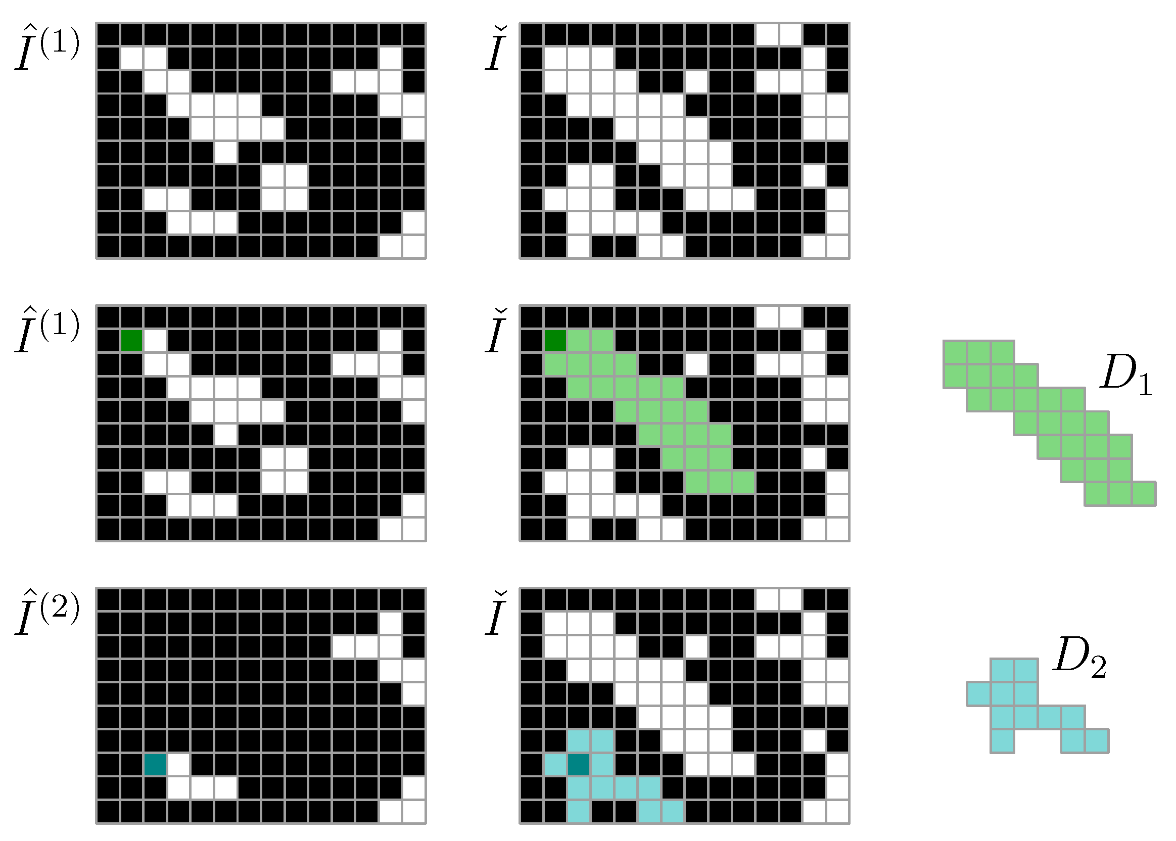
For image segmentation, we let be a threshold density for particle detection. To identify a particle, at least one of its pixel densities must exceed . Moreover, we let be a lower threshold density for particle detection. In this work, we use and . We consider only the kth density map . We let be a Boolean map of candidate particle positions, and we let indicate the set of pixels that may contain solids. To identify particle 1, first, we find one pixel such that is true. Then, we let be the set of all pixels found by a flood-fill operation on initiated at . This set of pixels is particle 1. We let , and then proceed to identify set of Particle 2, and so on (Figure 1). This is repeated across all images to identify all particles , , in the image stack.
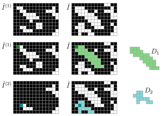
Figure 1.
Particle detection algorithm using high-threshold mask and low-threshold mask , where is used for floodfill particle domain detection. Each iteration (row) results in an identified particle domain , . The particle domains, with associated density weights , represent particles.
3.1.2. Particle Characterization
Particle is described by the pixels in its domain and the density of those pixels. For this particle, we introduce position vectors and densities , for some ordering of the pixels in .
The density sum of is
The average density of the particle is defined using the p norm,
Herein, we take so that approximates the maximum density. This yields a natural definition of particle area in units of px2,
We let be the empirical cumulative distribution function of densities in . The threshold density of particle , implied by our choice of particle area, is
Consequently, the number of pixels in such that is A. Conversely, Equation (10) can be written as . We define fibrillation index F as the negative of the derivative of the particle area with respect to the threshold, scaled by ,
where a preceding ‘d’ denotes the derivative of a function. By this definition, F quantifies the unsharpness of the particle–background interface.
To characterize the shape of the particle, we introduce an -degree polynomial,
with being the vector of polynomial coefficients. We also introduce rotated coordinates
with as the rotation angle. We let
be the weighted variance of the residuals of the polynomial. The backbone of the particle is now defined as
That is, the particle is rotated to produce the best possible weighted fit to a polynomial. With applied rotation , the interval spanned by the particle is with
The projected length of the particle is the Euclidean distance between its endpoints,
while the contour length is the arclength of the polynomial between its endpoints,
The natural definition of particle width is then
The geometry of the elongated particle is now defined, although we need to select order of the fitting polynomial. This is based on an estimate of aspect ratio for . A final fit is then carried out with
This may seem to be an arbitrary choice, but it is inspired by Sturges’ formula for choosing the number of bins in a histogram; with Sturges’ formula, the degrees of freedom of the histogram is with being the sample size. In our case, we envision r as the size, and as the degrees of freedom of the polynomial, which leads to Equation (20).
Page’s and Jordan’s curl index is [30]
To quantify the goodness of fit, we introduce the normalized variance,
This normalized variance takes large values if the particle has a re-entrant shape or if the particle is missing a single, well-defined backbone, as is the case for crossing fibers.
The curvature of the graph of q is defined as
with ‘’ as the second derivative, and the normalized maximum absolute curvature of the particle is
In the in-house characterization method, each particle is characterized by its contour length , width W, curl index C, fibrillation index F, average density , maximum absolute normalized curvature K, and normalized variance V. For reasons that become clear later (Section 3.2.1), we also include the redundant property , which gives a total of 8 parameters. Our physical interpretation of is that it represents the mean light attenuation of the particle. Notably, does not represent the centered backbone of the fiber, but the length of a fit polynomial, also W, is influenced by image density variations within the fiber, and is therefore not as exact as the caliper-like measures of commercial fiber analyzers. Moreover, the fibrillation measure quantifies the diffuseness of the particle–background interface and does not consider the actual geometry of fibrils. However, we stipulate that high accuracy may not be as important as high dimensionality for ML classification.
3.2. Machine Learning
In the following sections, the collection and preprocessing of data as well as four different ML algorithms are introduced: Lasso regression, support vector machine, feed-forward neural network and recurrent neural network. ML is evaluated through sensitivity (true positive rate, TPR) and specificity (true negative rate, TNR) which were calculated for each category, while accuracy (ACC) was calculated for each model.
where are the numbers of true positives, positives, true negatives, and negatives, respectively, and N is the sample size [31].
3.2.1. Data Processing
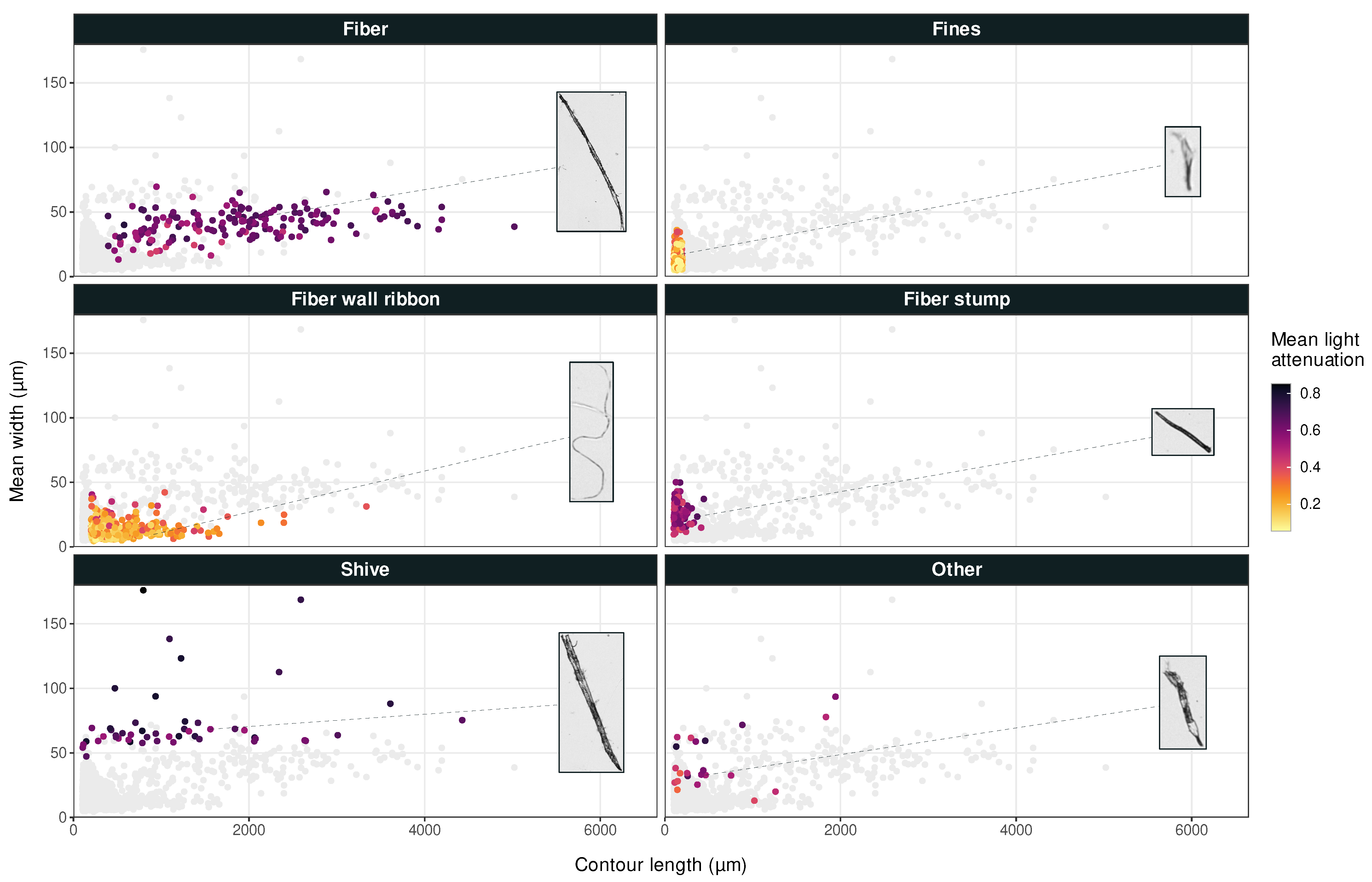
A graphical user interface was developed for manual classification of pulp objects. Based on images and parameters obtained from image analysis, specimens were classified by the user as either fiber, fines, fiber wall ribbon, fiber stump, shive, or other. Additionally, an object could be marked as clipped if it included an edge pixel of the raw micrographs, or cropped if it touched the edge of the single-object image from fiber analysis. Figure 2 shows example images for each class together with their location in scatter plots of the in-house image analysis dataset.
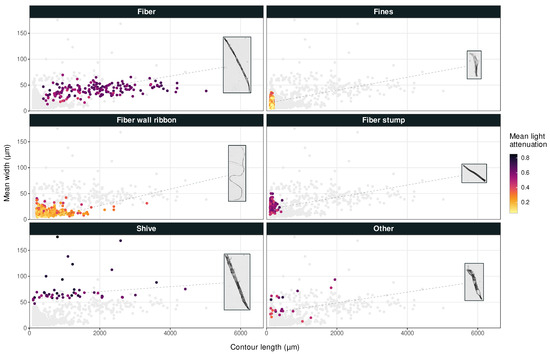
Figure 2.
Average width versus contour length for pulp particles, where each object is colored according to its mean light attenuation. Example images not to scale.
Dataset 1, obtained from L&W Fiber Tester plus, originally had 3332 objects, none of which were clipped or wider than 75 . After filtering out the cropped objects, it had 2354 observations, each one with 5 predictors.
Dataset 2 from the in-house image analysis software included 53,916 observations and was obtained from the same raw micrographs as Dataset 1. These datapoints were stratified using the Hartigan–Wong k-means algorithm [32]. Random samples of equal size were taken from each of the 12 strata and filtered from clipped objects. Moreover, 37 additional shives were weighted into the sample from the stratum with the widest particles, since this class was too small for ML. The result was 1391 observations, each one with 8 predictors.
Both datasets were preprocessed with the Yeo–Johnson transformation,
where parameter is identified through maximum likelihood estimation for each parameter of Datasets 1 and 2, respectively [33]. This transformation improves the symmetry and reduces the skewness of the distributions. Therefore, the performance of ML methods that benefit from near normality is enhanced.
Aside from Yeo–Johnson, two of the predictors in Dataset 2 were transformed into binary variables, reflecting certain classification criteria. Contour length was transformed so that
where the threshold of 200 is the industry standard for the maximum length of fines [3]. After this transformation, can no longer be calculated from the other parameters of Dataset 2, making it an independent variable. Another recurrent classification criterion is the distinction between light and dark objects. Mean light attenuation was transformed into binary variable , where a light and a dark bin were delimited by Ward’s hierarchical agglomerative clustering method. Murtagh’s Ward1 algorithm was applied to [34], and the resulting tree was cut into two branches, corresponding to the bins of . These transformations were expected to reduce collinearity between and , to eliminate outliers, and to reduce noise.
The ML algorithms were run on data both with and without Yeo–Johnson transformation preprocessing, and additionally on Dataset 2 without Yeo–Johnson, but with binary transformations. The proportion of training data was 0.8. Predictors and data are summarized in Table 1.

Table 1.
Summary of predictors and datasets.
3.2.2. Lasso Regression
The least absolute shrinkage and selection operator (Lasso) regression, or regularization, minimizes the residual sum of squares (RSS) subject to the Manhattan length of slope vector being lesser than some tuning parameter t [35]. In a standard linear model with predictors and responses , the Lasso estimators are
By Manhattan distance, or the norm, the unit circle is a lozenge, the unit sphere is an octahedron, and so on. Since the corners of an ball with radius t are situated on the coordinate axes and are more likely than its sides to intersect the RSS function, the models yield sparse solutions. This preference for zero slopes near the axes prevents overfitting and makes Lasso models stable, general, easy to interpret, and quick to compute [36,37]. If categorical response is modeled by multinomial distribution,
subject to the same constraint as in (30), where , are column vectors of coefficients, the maximum likelihood Lasso estimators can be approximated by coordinate descent. In this study, this was achieved using the glmnet package for R programming language [38,39].
3.2.3. Support Vector Machine
Support vector machine (SVM) is a non-parametric clustering algorithm that can be used for supervised ML for classification problems (SVC) and regression problems (SVR). The SVC algorithm is a classifier that finds an arbitrary hyperplane in N-dimensional space that partitions the data points into classes. The space between a hyperplane and the data points on each side of the hyperplane is called a margin and the data points closest to the margin span are so-called support vectors. The aim is to maximize the margin by finding the optimal hyperplane [40,41].
Linearly separable data can be classified using linear SVC directly on the data. For non-linearly separable data, however, the feature space needs to be transformed into higher dimensions using a kernel function, which allows for linear separation of the transformed data. The standard kernel is linear, and a commonly used kernel function is the Gaussian radial basis function (RBF). Aside from margin and kernels, other hyperparameters include regularization and the curvature of decision boundary . Adjusting alters the number of misclassified data points by the hyperplane and can prevent overfitting. For large values of , the data points are classified more accurately by allowing for a small-margin hyperplane, but this may lead to overfitting, while small values of could misclassify some data points to allow for large-margin hyperplanes. The hyperparameter determines the influence of each data point on the hyperplane. High values of consider only the hyperplane’s nearby data points, while small values of also consider data points farther away. The higher the value of , the more complex the hyperplane, which may lead to overfitting [40,41,42,43]. The SVM works effectively with data points with high margin separation and high-dimensional spaces and can be effective for large datasets and datasets with overlapping target classes [40,41].
In this work, an SVM implementation from the Scikit-learn open source library [44] was used with the linear or the RBF kernel, , and . Each combination was tested with each dataset to identify the optimal combination of highest total accuracy. Using these optimal parameters, sensitivity and specificity were calculated for each class.
3.2.4. Feed-Forward Neural Network
Feed-forward neural network (FFNN) models are comparatively simple and were among the earliest artificial neural networks developed for classification problems [45]. FFNN models process data with forward propagation, but update their model weights to minimize prediction errors using back propagation [46]. The neural network consists of neurons arranged in linear layers, where the first (the input layer) takes the parameters of the input data and the last (the output layer) outputs the classes. Between these two layers there is a hidden layer with an arbitrary number of neurons which identify and split the parameters in the input data to make a correct prediction for the output [45,47].
For the FFNN model, the influence of individual hyperparameters was investigated by varying each one in isolation. The model’s performance exhibits dependence on the quantity and nature of layers, the batch size that represents the number of independently processed samples, and the number of iterations over the same dataset, known as epochs. Additionally, the quantity of nodes within the hidden layers, the choice of activation function, and the optimizer selection contribute to the effectiveness of the model. In this study, we employed the Rectified Linear Unit (ReLU) as the activation function, which is a popular choice for computing values in the hidden layers of neural networks [13].
Three hyperparameters were varied in the model: batch size, epochs and number of nodes. The results from this variation were calculated by cross-entropy loss function, which displayed loss values for each epoch. This function is based on the probability distribution measurements obtained from the training results compared with the known classes. It can be described as the gap between the predicted categories and correct labels [45]. Optimization was achieved with stochastic gradient descent (SGD), which is the most common optimizer for updating parameters to minimize loss [48]. An FFNN implementation using PyTorch and Scikit Learn open source libraries [44,49] was used in this study.
3.2.5. Recurrent Neural Network
Recurrent neural networks (RNN) distinguish themselves from the conventionally used FFNNs by implementing a loop mechanism over each hidden layer. This facilitates the incorporation of previously acquired knowledge into every successive input [50].
The established problem of vanishing gradients refers to the known difficulty of RNNs to learn long-term dependencies, because the gradient of the result from the optimization algorithm tends to vanish or even explode [51,52]. Long short-term memory (LSTM) was designed solely to resolve this issue by introducing a recurrent unit, the so-called LSTM unit, into the RNN model. The LSTM unit possesses the dual capability to evaluate the significance of memories in relation to the output and to carry information over extended periods [53].
To address the issue of vanishing gradients, an alternative strategy was employed, which involved the introduction of a different recurrent unit referred to as the gated recurrent unit (GRU) [52]. GRU works similarly to LSTM; both models contain a gated recurring unit that regulates the exchange of information within the model. In contrast to LSTM, GRU delivers learned information without having a separate memory cell and without the ability to filter relevant memories from non-relevant ones [53].
Echoing the method outlined in Section 3.2.4, individual hyperparameters were systematically altered in the RNN model, with others held constant. These parameters encompassed epochs, batch size, activation functions, and node quantity per hidden layer. Sigmoid activation functions and hyperbolic tangent activation functions (Tanh), which are commonly used in neural networks, were, together with the previously mentioned ReLU, examined for each layer. In the final output layer, we utilized a softmax activation function, commonly employed for multinomial classification tasks [13]. The performance of the model was evaluated by calculating cross-entropy loss function, which was optimized using SGD. The RNN model was built with open-source software library Keras [54].
4. Results
4.1. Data Processing
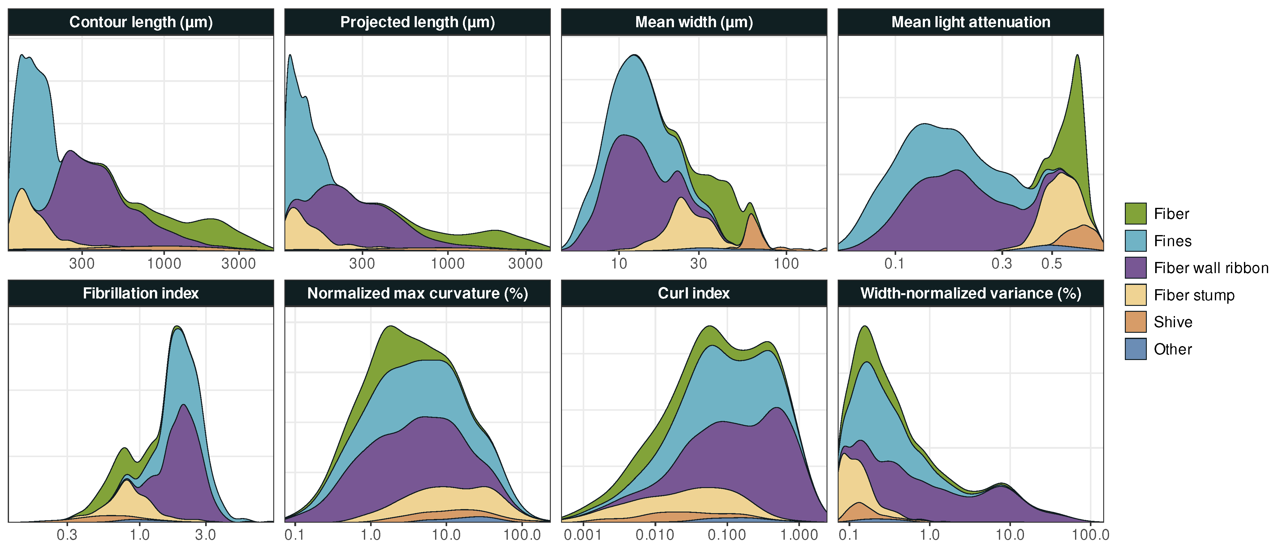
Particle class distributions for Dataset 2, smoothed with Gaussian kernel density functions using Silverman’s rule of thumb [55], are illustrated in Figure 3. Each class distribution in the contour length is essentially inside one of the bins of binary variable with its threshold at 200 . The two bins obtained using Ward’s method correspond to light attenuation ranges of 0.055 to 0.403, and 0.409 to 0.852, respectively, which is consistent with a partitioning local minimum of mean light attenuation distribution (Figure 3).
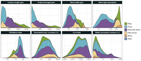
Figure 3.
The distribution of objects in each category for Dataset 2, smoothed with Gaussian kernel density functions to eliminate noise.
We observe that the properties of certain types of objects are more clearly distinguishable than others. For instance, fiber stumps and fines are both short, i.e., have relatively small contour lengths, but fiber stumps have much higher light attenuation, which makes the two object classes roughly distinguishable from binary variables alone. In contrast, the distinction between, e.g., fibers and shives requires consideration of interaction effects.
4.2. Machine Learning
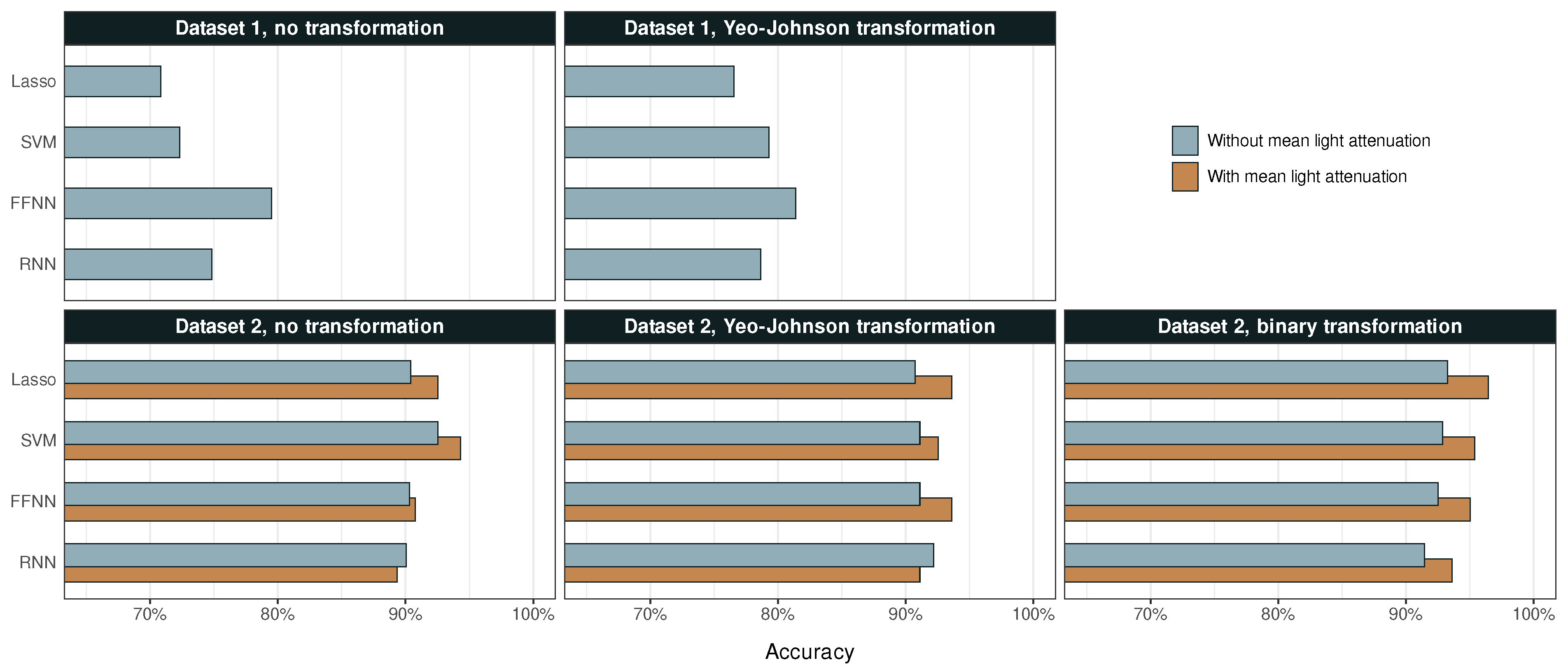
The accuracy of the different ML methods is summarized in Figure 4, while sensitivity and specificity are compiled in Table 2 and Table 3, respectively. Predictions of Dataset 1 have an accuracy of 71% to 81%, and the corresponding percentages for Dataset 2 are 89% to 96%. Another noteworthy difference shown in Table 2 is that the predictions of Dataset 2 have around three times higher sensitivity to shives than those of Dataset 1, even though this class is similarly sized in both sets.
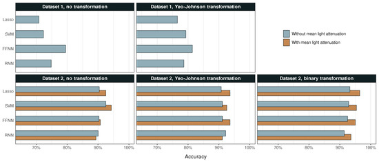
Figure 4.
The accuracy of each ML model for Datasets 1 and 2 before and after their respective transformations.
Table 2.
Statistics by class: Sensitivity. Sorted by descending accuracy.
Table 3.
Statistics by class: Specificity. Sorted by descending accuracy.
The predictions for Dataset 1 significantly improved after the Yeo–Johnson transformation, which indicates a high skewness in the original data. In general, neural networks seem to perform better than linear models on the L&W Fiber Tester plus built-in data analysis. FFNN achieved highest accuracy with 81%.
Despite its smaller size and lesser number of exact measurements of particle dimensions, Dataset 2 enables considerably more accurate classification. For non-transformed data, particularly including predictor , linear models perform better than neural networks. After Yeo–Johnson transformation, there is a slight increase in the accuracy of three models, but a decrease in accuracy of SVM. After binary transformations, however, all models produce more accurate predictions. The addition of has an unambiguous and similarly sized positive effect on accuracy across all models. Top accuracy is achieved by Lasso regression with 96%.
4.2.1. Lasso Regression
After scaling and centering the untransformed Dataset 2, neglecting the categories shive and other, the top three predictors ranked by absolute coefficient value were , , and . After binary encoding, the corresponding predictors were , , and V. Regularization did not improve accuracy, i.e., plain multinomial regression would have produced similar results.
4.2.2. Support Vector Machine
The optimal combination of kernel function and hyperparameters, , varied depending on the datasets being used (Table 4).
Table 4.
Optimal combination of hyperparameters for SVC.
4.2.3. Feed-Forward Neural Networks
Results for the FFNN model were obtained from runs with 10,000 epochs. Although the program became slower with such a large number of epochs, the accuracy became significantly higher, and this was deemed more important than short runtime. The hidden layer imported a tensor of size 64 from the first layer and exported a tensor of size 128 to the last layer. The number of classes was chosen to be six, in accordance with the number of particle categories.
4.2.4. Recurrent Neural Networks
For the RNN model, the optimal parameters used are presented in Table 5. The model consists of six different layers; two reshaping layers intended to reshape the data into proper format for processing, one LSTM layer, two different GRU layers and one output layer. The latter, which was used for final classification, was configured with 90 epochs and a batch size of 32, in accordance with Section 3.2.5, since this was predicted to be most efficient.
Table 5.
Optimal hyperparameters for the RNN model.
4.3. Figures, Tables and Schemes
5. Discussion
5.1. Image Analysis and Data Processing
Initially, Dataset 1 had no objects wider than 75 and no objects traversing the edges of the original pulp suspension micrographs. However, 978 of 3332 objects or 29% were classified as cropped and filtered out; these were predominantly particles with low contrast against the background, i.e., fiber wall ribbons and fines. In comparison, none of the 1391 objects in Dataset 2 were cropped. This is likely to introduce sampling bias toward dark objects in Dataset 1. Furthermore, the sample size difference causes selection bias; all available data points were used in Dataset 1, whereas Dataset 2 was the result of stratified sampling. Considering these biases in conjunction with the natural composition of the pulp, the predictors in Dataset 1 were expected to be highly skewed, which was confirmed by a significant increase in accuracy after the Yeo–Johnson transformation.
Figure 2 implies two sub-populations of shives when considering particle width distribution: one that is normally distributed around a regression line just below , and one smaller group of randomly scattered wider particles. The L&W Fiber Tester plus automatically discards objects with as shives [3]. This likely reduces the sensitivity of the shive category in Dataset 1, since the widest and most easily characterized particles were removed.
Due to the relatively small size of Dataset 2, some additional shives were included to facilitate ML, which somewhat skewed the distributions of W, and F. Since the bulk of this dataset is the product of equally allocated stratified sampling, it should have few other sources of skewness, which is supported by the somewhat ambiguous results of the Yeo–Johnson transformation.
Binary encoding alters the distribution of , eliminating the perfect multicollinearity involving C, and , yielding an additional independent predictor. It also reduces bias in , stemming from over-allocation of shives in stratified sampling. Finally, it reduces noise, which makes data easier to interpret and generates better and more uniform results across different types of models. A classification strategy with a stronger focus on quantitative category limits could arguably further facilitate encoding of predictors on binary or ordinal scales while improving consistency and repeatability. However, such a strategy is only recommended for pulps for which marginal distributions exhibit local minima.
5.2. Machine Learning
All four ML techniques were robust and were able to predict the desired classifications at a high accuracy. ML algorithms achieved higher accuracy when light attenuation predictors, or , were included. With transformed data, i.e., after preprocessing of Dataset 2, all methods produced better results by including light attenuation predictor . With non-transformed data, three out of four methods produced better results by including the corresponding light attenuation predictor . Only RNN deviated slightly from the observed positive trend, which is probably because it is more sensitive to outliers such as those observed for shives in Figure 2. However, for both RNN and FFNN, the effect of on non-transformed data was so small that it cannot be ruled out as a coincidence. The influence of light attenuation was only assessed for Dataset 2, since these parameters were only included in the in-house image analysis program.
For all ML methods, the general trend was that both the accuracy and the sensitivity increased when the Yeo–Johnson transformation was applied on Dataset 1 (Table 2). According to Figure 4, the methods that yielded largest improvements in accuracy when applying Yeo–Johnson transformations on Dataset 1 with light attenuation were SVM and FFNN methods. However, this trend cannot be seen for Dataset 2, for which SVM yielded lower accuracy after transformation than before. More exceptions could be observed for the RNN method and for shive and other categories, which sometimes showed a decrease in sensitivity. This trend can be correlated to the shapes of marginal distribution functions for shives and other in Appendix A (Figure A1, Figure A2 and Figure A3). These two categories exhibit more than one peak, whereas the other categories generally only have one. This indicates that shive and other were not favored by being treated as one population, whereas the remaining categories were. The RNN method, which sometimes produced results opposite to the general trend, could eventually be more sensitive to such tendencies. This unconfirmed hypothesis is corroborated by the observation that such deviating trend was not observed when (binary) transformations were applied on Dataset 2.
According to Figure 4, the binary transformation of Dataset 2 yielded highest accuracies for all four ML methods (with ), reaching an accuracy of 96% with Lasso regression. For both the binary and the Yeo–Johnson transformation of Dataset 2 (with ), the greatest improvement in accuracy was observed for FFNN.
Without transformations, the neural network methods (RNN and FFNN) performed better than the linear models (SVM and Lasso) on Dataset 1 but worse on Dataset 2. We believe that this tendency is due to the removal of objects wider than 75 from the former and the addition of such objects to the latter dataset. After binary transformations of and , this effect disappears.
The optimal kernels for Dataset 1, with and without the Yeo–Johnson transformation, were the linear kernel and the Gaussian RBF kernel, respectively. This was a consequence of the skewness of the data, as observed in Table 4.
When comparing the accuracy without the light attenuation parameter (cyan bars in Figure 4), it is a reasonable assumption that the difference observed between Datasets 1 and 2 cannot only be explained by the number of independent predictors, nor can this difference be explained by the amount of data or by the models themselves. It is rather data quality in conjunction with the number of predictors that contribute to the higher accuracy obtained with Dataset 2. At the cost of computational efficiency, the in-house image analysis model generates a larger and less skewed population of images, which allows for random, stratified sampling. In addition, the light attenuation predictor lends itself to a binary transformation, which seems to be highly conducive to ML.
5.3. Future Investigations
A suggestion for improving in-house image analysis is to adapt the polynomial functions to detect more objects and minimize the fraction of cropped images. Further investigation of adaptation could be conducted by selecting a polar coordinate system for the polynomial function in cases of re-entrant structures, or to split the polynomial into multiple polynomial segments when the variance becomes greater than some threshold value.
The category ’other’ contains objects that are of importance for the pulp and paper industry, and can therefore be divided into other industry informative categories such as fiber flake, ray cell, fibril, and pore. This would likely improve accuracy in ML, since the skew in the input would be reduced. Such subdivision would, however, require a much greater set of training data. It could also be useful to split the category shive into smaller categories in order to increase its sensitivity and thereby reach a level comparable to that of the other categories.
For all algorithms, the highest sensitivity values were obtained for Dataset 2 with binary transformations. These results indicate that methods where binary characteristics are assigned as parameters instead of numerical values, for example, multi-view clustering or crossed categorization, could improve ML for pulp and paper characterization. The possibility to use binary transformations, however, hinges on the presence of bimodal features in the marginal distributions of individual classes.
Furthermore, it could also be useful to apply ML directly to the pictures, since this would eliminate the requirement of using a separate image analysis program to process and calculate object parameters. This could be achieved using the four tested ML methods, but other techniques could also be utilized, such as the k-nearest neighbors (KNN) ML method.
6. Conclusions
All four assessed ML techniques performed very well and reached accuracies in the range of 94% to 96% when optimal settings and input data from the in-house image analysis program were used. These results confirm that (on-line) image analysis of fiber suspensions, combined with modern ML techniques, can become a fast and cost-efficient tool for the industry to assess improved quality control of fiber materials.
Data obtained with the in-house image analysis software, which included an important light attenuation parameter, generally offered improved ML accuracy compared to the dataset with conventional pulp particle characterization intended for engineer users. This is to a large extent due to the extended parameter set provided by the in-house software, which should be straightforward to include in commercial fiber analyzers to provide robust, automated particle classification.
Preprocessing of the data with either the Yeo–Johnson transformation or binary transformations also improved the accuracy for all ML algorithms and datasets. After transformation, the FFNN method displayed the highest accuracy, 81%, for the datasets obtained with the built-in software of the fiber analyzer, whereas Lasso regression showed the best accuracy, 96%, for the in-house image analysis software.
Author Contributions
Conceptualization, R.A., E.G., L.A., M.K., S.B.L., J.P. and F.N.; methodology, R.A., E.G., L.A., M.K., S.B.L. and F.N.; software, R.A., E.G., L.A., M.K. and S.B.L.; validation, R.A., E.G., L.A. and M.K.; formal analysis, R.A., E.G., L.A., M.K. and S.B.L.; investigation, R.A., E.G., L.A., M.K., K.L., J.P. and J.-E.B.; data curation, F.N.; writing—original draft preparation, R.A., E.G., L.A., M.K. and S.B.L.; writing—review and editing, R.A., E.G., L.A., M.K., K.L., J.P., J.-E.B., B.A.E. and F.N.; visualization, M.K. and S.B.L.; supervision, F.N.; project administration, B.A.E.; funding acquisition, B.A.E. All authors have read and agreed to the published version of the manuscript.
Funding
The work was carried out within the Strategic Innovation Program for Process Industrial IT and Automation, a joint initiative by Vinnova, Formas, and the Swedish Energy Agency, as Vinnova grant agreement No. 2022-03597. The work was conducted within the research profile Neopulp financed by the Knowledge foundation. S. B. Lindström thanks Svenska Cellulosa AB (SCA) for financial support. The support from “FibRe—A Competence Centre for Design for Circularity: Lignocellulose-based Thermoplastics”, partly funded by the Swedish Innovation Agency VINNOVA (Grant Number 2019-00047), is also sincerely acknowledged.
Data Availability Statement
The data presented in this study are available in article.
Acknowledgments
The authors thank Holmen AB for supplying pulp samples. We are also indebted to ABB for kindly providing and supporting the L&W Fiber Tester plus fiber analyzer.
Conflicts of Interest
The authors declare no conflict of interest.
Appendix A
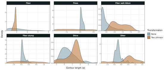
Figure A1.
Probability density versus particle contour length in Dataset 1.
Figure A1.
Probability density versus particle contour length in Dataset 1.

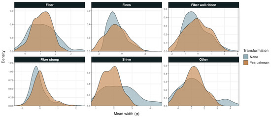
Figure A2.
Probability density versus mean particle width in Dataset 1.
Figure A2.
Probability density versus mean particle width in Dataset 1.


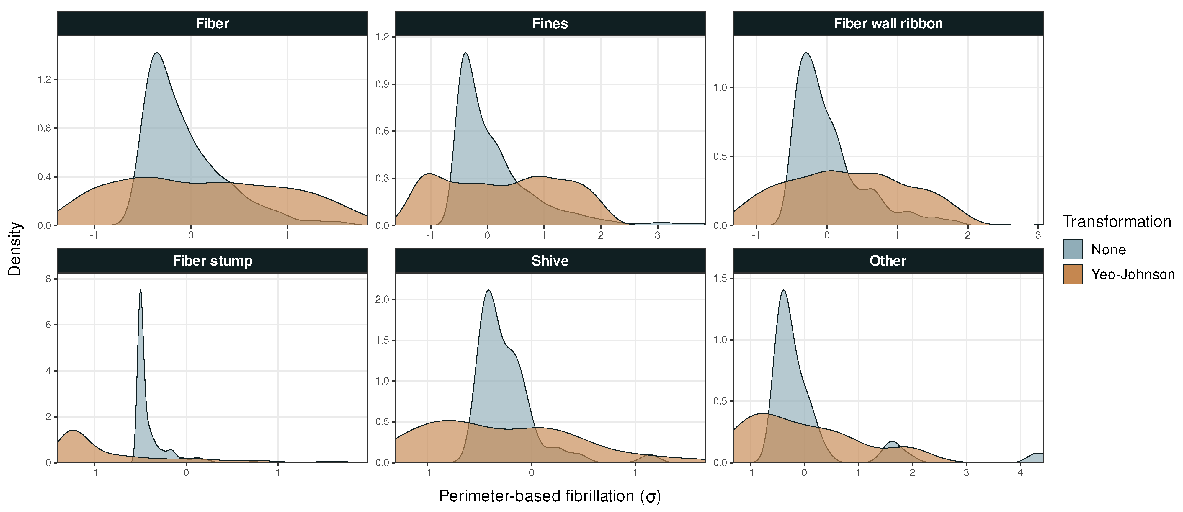
Figure A3.
Probability density versus perimeter-based fibrillation in Dataset 1. Outliers removed from the fines and fiber stump panels.
Figure A3.
Probability density versus perimeter-based fibrillation in Dataset 1. Outliers removed from the fines and fiber stump panels.
References
- Dannelly, W. Advancements in Fiber Analysis Techniques: The Future of Improving Pulp Quality. 2021. Available online: https://library.e.abb.com/public/7320c5d8f04a48daa4580229f39c93a5/Future%20of%20Fiber_PPL_SeptOct21.pdf (accessed on 30 March 2023).
- FSCN Research Centre. NeoPulp. Available online: https://www.miun.se/Forskning/forskningsprojekt/pagaende-forskningsprojekt/neopulp (accessed on 1 June 2023).
- Karlsson, H. Fibre Guide—Fibre Analysis and Process Applications in the Pulp and Paper Industry; AB Lorentzen & Wettre: Kista, Sweden, 2006; pp. 5–8, 51–68. [Google Scholar]
- Österholm, H. Fiber analysis with online and virtual measurements enables new closed loop control strategies for pulp quality. Pulp Pap. Logist. 2021, 12, 10–13. [Google Scholar]
- Aronsson, M. On 3D Fibre Measurements of Digitized Paper from Microscopy to Fibre Network. Ph.D. Thesis, Swedish University of Agricultural Sciences, Uppsala, Sweden, 2002. [Google Scholar]
- Axelsson, M. Image Analysis for Volumetric Characterisation of Microstructure. Ph.D. Thesis, Swedish University of Agricultural Sciences, Centre for Image Analysis, Uppsala, Sweden, 2009. [Google Scholar]
- Paciornik, S.; d’Almeida, J. Digital microscopy and image analysis applied to composite materials charecterizaation. Rev. Matér. 2010, 15, 172–181. [Google Scholar] [CrossRef]
- Murphy, K.P. Machine Learning: A Probabilistic Perspective; MIT Press: Cambridge, MA, USA, 2012; pp. 1–19. [Google Scholar]
- Pandey, M.E.; Rautaray, S.S.E. Machine Learning: Theoretical Foundations and Practical Applications; Springer: Singapore, 2021; pp. 57–87. [Google Scholar]
- Salvador, J. Example-Based Super Resolution; Elsvier: Amsterdam, The Netherlands, 2017; pp. 113–127. [Google Scholar]
- Donaldson, L. Analysis of fibres using microscopy. In Handbook of Textile Fibre Structure Fundamentals and Manufactured Polymer Fibres, 1st ed.; Woodhead Publishing: Scion, New Zealand, 2009; Chapter 4; pp. 121–153. [Google Scholar]
- Berg, P.; Lingqvist, O. Pulp, Paper, and Packaging in the Next Decade: Transformational Change; McKinsey & Company: Chicago, IL, USA, 2019; Available online: https://www.mckinsey.com/industries/packaging-and-paper/our-insights/pulp-paper-and-packaging-in-the-next-decade-transformational-change (accessed on 30 March 2023).
- Goodfellow, I.; Bengio, Y.; Courville, A. Deep Learning; The MIT Press: Cambridge, MA, USA, 2016; pp. 163–168, 775. [Google Scholar]
- Kalavathi Devi, T.; Priyanka, E.; Sakthivel, P. Paper quality enhancement and model prediction using machine learning techniques. Results Eng. 2023, 17, 100950. [Google Scholar] [CrossRef]
- Nisi, K.; Nagaraj, B.; Agalya, A. Tuning of a PID controller using evolutionary multi objective optimization methodologies and application to the pulp and paper industry. Int. J. Mach. Learn. Cybern. 2019, 10, 2015–2025. [Google Scholar] [CrossRef]
- Jauhar, S.; Raj, P.; Kamble, S.; Pratap, S.; Gupta, S.; Belhadi, A. A deep learning-based approach for performance assessment and prediction: A case study of pulp and paper industries. Ann. Oper. Res. 2022, 2022, 1–27. [Google Scholar] [CrossRef]
- Narciso, D.A.; Martins, F. Application of machine learning tools for energy efficiency in industry: A review. Energy Rep. 2020, 6, 1181–1199. [Google Scholar] [CrossRef]
- Othen, R.; Cloppenburg, F.; Gries, T. Using machine learning to predict paperboard properties—A case study. Nord. Pulp Pap. Res. J. 2022, 38, 27–46. [Google Scholar] [CrossRef]
- Parente, A.; de Souza, M., Jr.; Valdman, A.; Folly, R. Data Augmentation Applied to Machine Learning-Based Monitoring of a Pulp and Paper Process. Processes 2019, 7, 958. [Google Scholar] [CrossRef]
- Talebjedi, B.; Laukkanen, T.; Holmberg, H.; Vakkilainen, E.; Syri, S. Energy simulation and variable analysis of refining process in thermo-mechanical pulp mill using machine learning approach. Math. Comput. Model. Dyn. Syst. 2021, 27, 562–585. [Google Scholar] [CrossRef]
- Talebjedi, B.; Laukkanen, T.; Holmberg, H.; Vakkilainen, E.; Syri, S. Advanced energy-saving optimization strategy in thermo-mechanical pulping by machine learning approach. Nord. Pulp Pap. Res. J. 2022, 37, 434–452. [Google Scholar] [CrossRef]
- ISO 5263-3:2023, IDT; Pulps—LaboratoryWet Disintegration—Part 3: Disintegration of Mechanical Pulps at ≥85 °C. International Organization for Standardization: Geneva, Switzerland, 2023.
- ABB. L&W Fiber Tester Plus Testing and Industry-Specific Instruments; ABB Group: Kista, Sweden, 2020. [Google Scholar]
- ISO 16065-2:2014, IDT; Pulps—Determination of Fibre Length by Automated Optical Analysis—Part 2: Unpolarized Light Method. International Organization for Standardization: Geneva, Switzerland, 2014.
- Fiber Length of Pulp and Paper by Automated Optical Analyzer Using Polarized Light, Test Method TAPPI/ANSI T 271 om-23; Technical Association of the Pulp and Paper Industry: Atlanta, GA, USA, 2023.
- Hyll, K.; Farahari, F.; Mattson, L. Optical Methods for Fines and Filler Size Characterization: Evaluation and Comparison; Technical report; Innventia: Stockholm, Sweden, 2016. [Google Scholar]
- Fiber Length of Pulp by Projection, Test Method TAPPI T 232 cm-23; Technical Association of the Pulp and Paper Industry: Atlanta, GA, USA, 2023.
- Fiber Length of Pulp by Classification, Test Method TAPPI T 233 cm-15; Technical Association of the Pulp and Paper Industry: Atlanta, GA, USA, 2015.
- ISO 16065-1:2014, IDT; Pulps—Determination of Fibre Length by Automated Optical Analysis—Part 1: Polarized Light Method. Standard, International Organization for Standardization: Geneva, Switzerland, 2014.
- Page, D.H.; Seth, R.S.; Jordan, B.D.; Barbe, M. Curl, crimps, kinks and microcompressions in pulp fibres—their origin, measurement and significance. In Papermaking Raw Materials, Trans. of the VIIIth Fund. Res. Symp. Oxford; Punton, V., Ed.; FRC: Manchester, UK, 1985; pp. 183–227. [Google Scholar] [CrossRef]
- Altman, D.G.; Bland, J.M. Statistics Notes: Diagnostic tests 1: Sensitivity and specificity. Br. Med. J. 1994, 308, 1552. [Google Scholar] [CrossRef] [PubMed]
- Hartigan, J.A.; Wong, M.A. A k-means clustering algorithm. J. R. Stat. Soc. Ser. Appl. Stat. 1979, 28, 100–108. [Google Scholar]
- Yeo, I.K.; Johnson, R. A new family of power transformations to improve normality or symmetry. Biometrika 2000, 87, 954–959. [Google Scholar] [CrossRef]
- Murtagh, F.; Legendre, P. Ward’s hierarchical agglomerative clustering method: Which algorithms implement Ward’s criterion? J. Classif. 2014, 31, 274–295. [Google Scholar] [CrossRef]
- Tibshirani, R. Regression Shrinkage and Selection Via the Lasso. J. R. Stat. Soc. Ser. Stat. Methodol. 1996, 58, 267–288. [Google Scholar] [CrossRef]
- Yuan, G.X.; Chang, K.W.; Hsieh, C.J.; Lin, C.J. A Comparison of Optimization Methods and Software for Large-scale L1-regularized Linear Classification. J. Mach. Learn. Res. 2010, 11, 3183–3234. [Google Scholar]
- Hastie, T.; Tibshirani, R.; Wainwright, M. Statistical Learning with Sparsity; CRC Press: Boca Raton, FL, USA, 2015; pp. 1–3, 23–24. [Google Scholar]
- Friedman, J.H.; Hastie, T.; Tibshirani, R. Regularization Paths for Generalized Linear Models via Coordinate Descent. J. Stat. Softw. 2010, 33, 1–22. [Google Scholar] [CrossRef]
- Tay, J.K.; Narasimhan, B.; Hastie, T. Elastic Net Regularization Paths for All Generalized Linear Models. J. Stat. Softw. 2023, 106, 1–31. [Google Scholar] [CrossRef]
- Ben-Hur, A.; Horn, D.; Siegelmann, H.T.; Vapnik, V. Support Vector Clustering. J. Mach. Learn. Res. 2001, 2, 125–137. [Google Scholar] [CrossRef]
- Gholami, R.; Fakhari, N. Handbook of Neural Computation; Academic Press: Cambridge, MA, USA, 2017; pp. 515–535. [Google Scholar] [CrossRef]
- Pisner, D.A.; Schnyer, D.M. Machine Learning; Academic Press: Cambridge, MA, USA, 2020; pp. 101–121. [Google Scholar] [CrossRef]
- Schölkopf, B.; Smola, A. Learning with Kernels: Support Vector Machines, Regularization, Optimization and Beyond; MIT Press: Cambridge, MA, USA, 2002. [Google Scholar]
- Pedregosa, F.; Varoquaux, G.; Gramfort, A.; Michel, V.; Thirion, B.; Grisel, O.; Blondel, M.; Prettenhofer, P.; Weiss, R.; Dubourg, V.; et al. Scikit-learn: Machine Learning in Python. J. Mach. Learn. Res. 2011, 12, 2825–2830. [Google Scholar]
- Zhou, X.; Liu, H.; Shi, C.; Liu, J. The basics of deep learning. In Deep Learning on Edge Computing Devices; Elsevier: San Diego, CA, USA, 2022; Chapter 2; pp. 19–36. [Google Scholar]
- Rumelhart, D.E.; Hinton, G.E.; Williams, R.J. Learning representations by back-propagating errors. Nature 1986, 323, 533–536. [Google Scholar] [CrossRef]
- Svozil, D.; Kvasnicka, V.; Pospichal, J. Introduction to multi-layer feed-forward neural networks. Chemom. Intell. Lab. Syst. 1997, 39, 43–62. [Google Scholar] [CrossRef]
- Ketkar, N. Stochastic Gradient descent. In Deep Learning with Python: A Hands-on Introduction; Apress: Berkeley, CA, USA, 2017; pp. 113–132. [Google Scholar]
- Paszke, A.; Gross, S.; Massa, F.; Lerer, A.; Bradbury, J.; Chanan, G.; Killeen, T.; Lin, Z.; Gimelshein, N.; Antiga, L.; et al. PyTorch: An Imperative Style, High-Performance Deep Learning Library. In Advances in Neural Information Processing Systems 32; Curran Associates, Inc.: Red Hook, NY, USA, 2019; pp. 8024–8035. [Google Scholar]
- Kostadinov, S. Recurrent Neural Networks with Python Quick Start Guide; Packt Puplishing: Kista, Sweden, 2018. [Google Scholar]
- Sherstinsky, A. Fundamentals of Recurrent Neural Network (RNN) and Long Short-Term Memory (LSTM) network. Phys. D Nonlinear Phenom. 2020, 404, 132306. [Google Scholar] [CrossRef]
- Hochreiter, S.; Schmidhuber, J. Long Short-Term Memory. Neural Comput. 1997, 9, 1735–1780. [Google Scholar] [CrossRef]
- Chung, J.; Gulcehre, C.; Cho, K.; Bengio, Y. Empirical evaluation of gated recurrent neural networks on sequence modeling. In Proceedings of the NIPS 2014 Workshop on Deep Learning, Montreal, QC, Canada, 13 December 2014. [Google Scholar]
- Chollet, F. Keras. 2015. Available online: https://github.com/fchollet/keras (accessed on 1 June 2023).
- Silverman, B.W. Density Estimation for Statistics and Data Analysis; Chapman & Hall: London, UK, 1986; p. 48. [Google Scholar]
Disclaimer/Publisher’s Note: The statements, opinions and data contained in all publications are solely those of the individual author(s) and contributor(s) and not of MDPI and/or the editor(s). MDPI and/or the editor(s) disclaim responsibility for any injury to people or property resulting from any ideas, methods, instructions or products referred to in the content. |
© 2023 by the authors. Licensee MDPI, Basel, Switzerland. This article is an open access article distributed under the terms and conditions of the Creative Commons Attribution (CC BY) license (https://creativecommons.org/licenses/by/4.0/).