Abstract
Digital soil maps are paramount for supporting environmental process analysis, planning for the conservation of ecosystems, and sustainable agriculture. The availability of dense time series of surface reflectance data provides valuable information for digital soil mapping (DSM). A detailed soil survey, along with a stack of Landsat 8 SR data and a rainfall time series, were analyzed to evaluate the influence of soil on the temporal patterns of vegetation greenness, assessed using the normalized difference vegetation index (NDVI). Based on these relationships, imagery depicting land surface phenology (LSP) metrics and other soil-forming factors proxies were evaluated as environmental covariates for DSM. The random forest algorithm was applied as a predictive model to relate soils and environmental covariates. The study focused on four soils typical of tropical conditions under pasture cover. Soil parent material and topography covariates were found to be similarly important to LSP metrics, especially those LSP images related to the seasonal availability of water to plants, registering significant contributions to the random forest model. Stronger effects of rainfall seasonality on LSP were observed for the Red Latosol (Ferralsol). The results of this study demonstrate that the addition of temporal variability of vegetation greenness can be used to assess soil subsurface processes and assist in DSM.
1. Introduction
A range of complex factors, such as soil-forming factor interaction and pedogenic processes, determines soil distribution across geographical regions. Digital maps in raster format currently represent soil-forming factors coined as environmental covariates [1]. The digital soil mapping (DSM) framework quantitatively integrates relationships between climate, vegetation patterns, and a geomorphological setting at the landscape level into a soil map [1,2]. A remarkable convergence of several geospatial information toward DSM has occurred, primarily due to the fast evolution of remote sensing products and increasing information on web-based platforms for easy access to an extensive catalog in a ready-to-use format. Historically, the most applied environmental covariates consist of a raster format representing the space of the current information rather them temporal variations [3,4] (Wadoux et al., 2021; Coelho et al., 2021). Since several geospatial data could be surrogates for soil-forming factors, new environmental covariates should be adequately evaluated and interpreted with caution when applied with machine learning algorithms to ensure their real meaningfulness concerning soil prediction [3].
Historically, pedologists have recorded and observed vegetation pattern information to support the spatial prediction of soil types on different scales [5]. Such soil–vegetation correlation is possible since spatial and temporal dynamics of vegetation serve as indicators of the interaction between soil conditions and climate regimes. Organisms and vegetation are dynamic soil-forming factors, and their relationship with climate and soil properties is vital, particularly with regard to factors that constrain plant growth and vigor, such as water availability and fertility [6,7].
Soil moisture regimes have been intensely monitored in developed countries, furnishing support for soil classification systems [8]. Conversely, the lack of country-based soil and climate monitoring on a detailed scale led pedologists to classify native vegetation with the purpose of soil mapping. In this case, plant deciduousness is the primary basis for making inferences about soil-hydric regimes [9]. However, native vegetation remnants for inferences have been increasingly scarce. Thus, there is an avenue to be explored by applying satellite-based vegetation indexes to increase the accuracy of information. In turn, soil information could aid vegetation index interpretations.
Reliable detection and mapping of plant dynamics can be achieved through remote sensing of vegetation greenness. This is because the spectral features of plants are closely tied to their biomass, yield, health, and vigor, making them a valuable metric for assessing greenness. The normalized difference vegetation index—NDVI—is the most commonly used index [10,11,12]. With the increasing availability of remote sensing and cloud-computing technology, continuous collections of satellite imagery can be used to add a temporal dimension to studies using spectral vegetation indexes [13,14]. Research on using temporal variability of vegetation indices in DSM has taken various approaches, including single-season analysis based on wet versus dry conditions [15] and analysis of time series of dense vegetation indexes [16,17].
The acquisition of satellite-based temporal vegetation indexes allows studies of seasonal patterns in plant phenophases, called land surface phenology (LSP) [10]. Considering a local-scale analysis, soil–landscape conditions drive plant changes in their coloring and leaf fall [18] (Caparros-Santiago et al., 2021), and climate drives the cycles of plants throughout the season [19] (Wolkovich et al., 2012). The rhythm of different phenological events has been considered a critical biological indicator [18] (Caparros-Santiago et al., 2021). Once related with soil types, LSP imagery can provide a valuable environmental covariate to enhance DSM. By utilizing LSP imagery related to vegetation growing seasons (such as season start and end, integrated NDVI, and seasonal amplitudes), information depicting the climate-driven cycles of vegetation greenness can be synthesized [20]. Despite the demonstrated feasibility of using LSP metrics for DSM predictive models for soil properties, such as organic carbon, sand, and calcium content [21,22], the impact of soil taxonomic class and its interaction with rainfall seasonality has been overlooked, particularly in tropical regions where data scarcity poses a challenge for detailed mapping.
This study aims to evaluate the use of LSP metrics for DSM as an effective environmental covariate, combined with relief and soil parent material proxies. The hypothesis tested is that the temporal variability of vegetation greenness is influenced by the interaction of soil and rainfall seasonality, producing a temporal signature that can be captured through remote observation to enhance DSM.
2. Materials and Methods
2.1. Study Area and Soil Survey
A comprehensive study of the soil in an area of 314 hectares located on the Campus of the Federal University of Lavras, Minas Gerais state, Brazil, was conducted. The soil sampling was carried out in a regularly spaced grid, with approximately 130 m of nearest neighbor distance between each sample [23] (Figure 1). The soils were sampled and described according to standard procedures outlined in an earlier paper [24], and chemical and physical analyses were carried out according to a previous study [25]. The soils were then classified according to the Brazilian soil classification system [24].
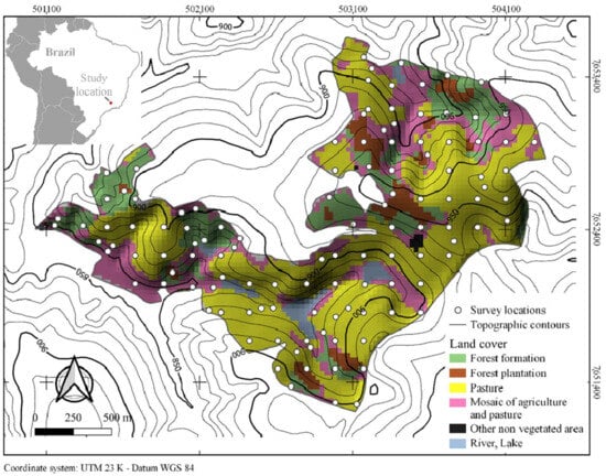
Figure 1.
Study area, land cover, and survey locations at Federal University of Lavras, Southern Minas Gerais state, Brazil. Topographic contours represent 10 m intervals.
The climate of the region is classified as Cwb, which is a humid tropical climate with a dry winter and temperate summer, according to Köppen’s classification criteria [26]. The vegetation cover in the area is a mosaic of pasture, native forest, forest plantation, and agriculture, as determined by data from the MapBiomas project (https://mapbiomas.org/ (accessed on 5 January 2020)). It was also found that there has been no significant change in land cover between the years 2012 and 2019 [27].
Overall, the study provides a detailed analysis of the soil in the area, which will be beneficial for future research and development projects on the Campus of the Federal University of Lavras.
2.2. Vegetation Greenness Time Series and Land Surface Phenology
We searched the Google Earth Engine database for all 168 scenes captured by the Landsat 8 OLI sensor between 19 April 2013 and 12 August 2020, using path 218 and row 75, for surface reflectance imagery. Unfortunately, 17 scenes were unavailable. The image collection has already undergone atmospheric correction and orthorectification, making it better suited for temporal analysis. We then cropped the selected collection to the study area for pasture land cover only. Finally, we calculated the NDVI proxy for vegetation greenness and scaled it using Equation (1):
where NIR is near-infrared surface reflectance (band 5) and R is red surface reflectance (band 4). The factor of 104 was applied for more efficient use of memory. Image cropping and NDVI calculation were performed in the raster package [28] in the R platform [29].
The LSP metrics were obtained using the TIMESAT algorithm [30], which was specifically designed for extracting seasonal parameters from optical remote sensing vegetation indices. TIMESAT uses seasonal models such as asymmetric Gaussian functions, double logistic, and the Savitzky–Golay filter. The process of selecting and fitting the seasonal models was iterative and involved visual interpretation and reference checks with NDVI literature values [20,30]. To accomplish this, the temporal stack of NDVI images derived from Landsat 8 imagery was analyzed using TIMESAT.
The primary source of noise in the temporal signal of NDVI is caused by the occurrence of clouds and shadows, generating a negatively biased noise [31]. To address this, a weighted least-squares approach was implemented in TIMESAT. This involved assigning higher weights to high NDVI values in the time series to construct an upper envelope of data, which was used to fit the seasonal model [20,30]. In cases where Landsat 8 scenes were completely cloud-covered or had unavailable dates, they were treated as “no data” and excluded from input into TIMESAT.
Thirteen different LSP maps were obtained for each season: season start time, season end time, season length, NDVI base level, season mid-time, largest NDVI value for the fitted function, seasonal amplitude, rate of increase at the beginning of the season, rate of decrease at the end of the season, large seasonal integral, small seasonal integral, NDVI value for the start of the season, and NDVI value for the end of the season [20,30].
2.3. Additional Soil Environmental Covariates: Topography and Parent Material
Considering the scale of analysis and the most important drivers of soil formation, maps depicting topography and soil parent material were also evaluated. SAGA-GIS [32] was used to derive terrain attributes commonly used in DSM applications based on a 5 m resolution DEM (digital elevation model), which was interpolated by the ANUDEM method from topographic contours of 1 m of vertical distance [33]. Besides DEM, the following terrain attributes were also calculated: slope, diffuse insolation, direct insolation, saga wetness index (SWI), stream power index (SPI), topographic position index (TPI), multiresolution valley bottom flatness (MRVBF), and multiresolution ridge top flatness index (MRRTF).
Despite the lack of a detailed geological map for the study region, we were able to generate soil parent material proxies using proximal sensor data and knowledge of soil–geology relationships. Silva et al. [34] and Curi et al. [23] interpreted magnetic susceptibility from B and C soil horizons of the same area to generate spatial information about soil parent material. Magnetic susceptibility was measured using a Barrington MS2B magnetometer (Bartington Instruments Co., Ltd., Oxford, UK) at low frequency. We resampled all soil covariates to match the spatial resolution of the Landsat 8 data (30 m).
In addition to magnetic susceptibility, soil texture, obtained by the pipette method [35], and soil organic matter, determined by wet oxidation [25], were also obtained from Curi et al. [23] and were used to support additional analyses.
2.4. Digital Soil Mapping
After harmonizing and gathering the environmental covariates, the complete framework of DSM was established, as displayed in Equation (2):
Soil classes = f (LSP metrics, topography, parent material) + Ɛ
Climate and organisms were considered spatial constants due to the scale of this study. Thus, the soil classes were spatially associated (f) with environmental covariates through a random forest algorithm [30,31]. Random forest [36,37] is currently one of the most applied machine learning algorithms in soil science due to its remarkable performance of bootstrapping and bagging features to reveal patterns in complex soil spatial association [38,39,40]. This non-parametric data-driven model has obtained accurate soil predictions even when based on many environmental covariates [41]. Random forest parameterization followed the approach proposed by Hengl et al. [38]: mtry = 5 (an approximate integer of the square root of the number of covariates, i.e., 30) and ntrees = 500 (number of trees sufficient to fit a model) [37]. To ensure adequate sample size, only soil classes with at least six records or samples under pasture vegetation cover were analyzed. These included Haplic Cambisol, Red Latosol, Red-Yellow Latosol, and Red-Yellow Argisol (soils classified according to Santos et al. [24]). According to Soil Survey Staff [42], those soil types correspond to Typic Dystrudept, Rhodic Hapludox, Typic Hapludox, and Typic Hapludult, respectively. Additionally, according to the World Reference Base for Soil Resources [43] (IUSS Working Group WRB, 2015), those soils respectively correspond to Cambisol, Ferralsol, and Acrisol.
The accuracy (Ɛ) associated with the spatial prediction model was assessed using repeated 5-fold cross-validation allowing the calculation of global accuracy and the kappa index [44] statistical metrics.
Random forest is referred as a “black box” model [45] because it is difficult to understand how model inputs and environmental covariates are combined to make the final prediction. To improve the interpretability of the models and uncover patterns, the rank of variable importance was obtained by the mean decrease in classification accuracy calculated globally and for each soil taxonomic class [36]. Permuting the environmental covariate values that might increase the prediction error could be interpreted as a score of importance. A higher score indicated a more critical environmental covariate due to its significant effect on the prediction.
2.5. Rainfall Seasonality
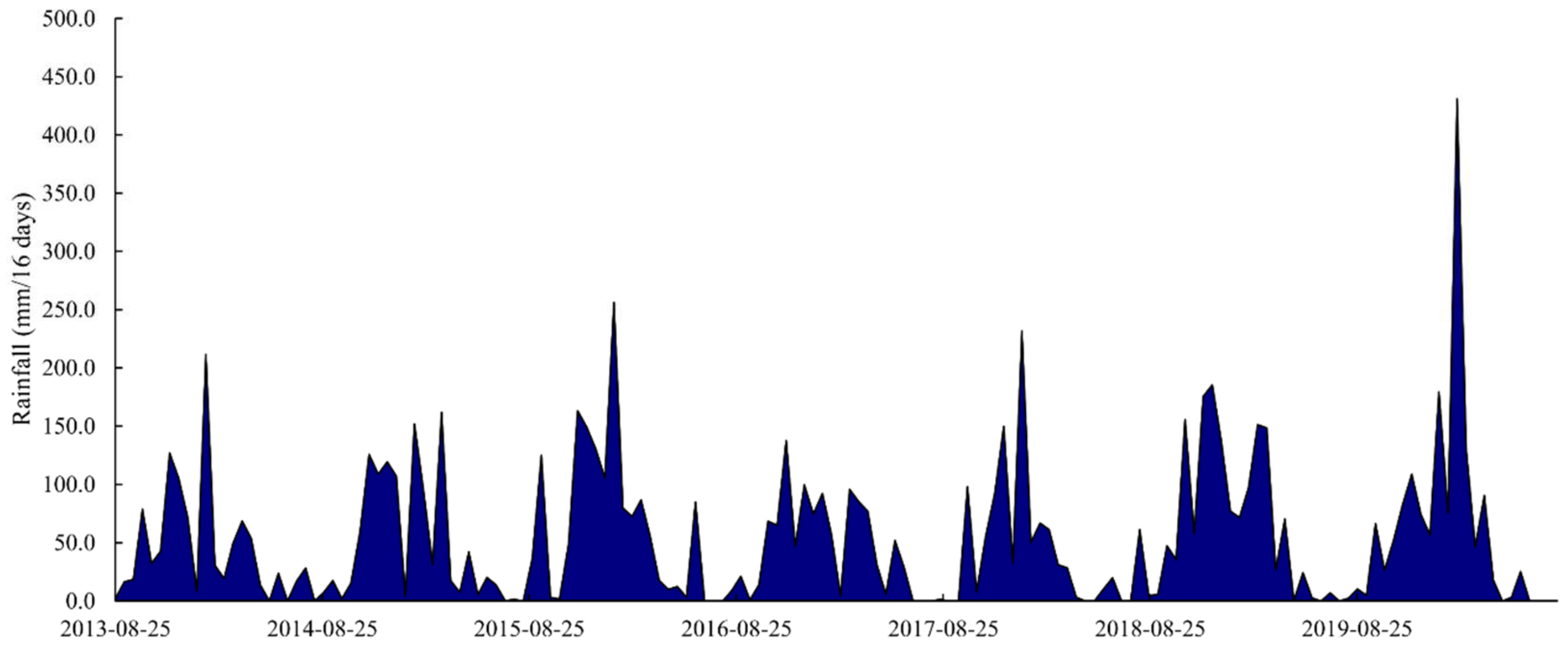
A time series of rainfall was built from daily precipitation data from the 83687 BDMEP—INMET station, available at http://www.portal.inmet.gov.br (accessed on 10 January 2020). The daily data were combined to match the temporal resolution and dates of the NDVI time series, meaning that daily rainfall data were accumulated over 16-day periods (Figure 2). Using TIMESAT, an analysis of the rainfall time series allowed for the identification of seven seasons. Consequently, the initial image collection was filtered to match these periods.

Figure 2.
Time series of aggregated 16-days rainfall for the study area (date format: year-month-day).
Finally, Spearman’s rank correlation analysis was performed between the most important LSP covariate ranked from random forest importance scores and the accumulated seasonal rainfall at each soil class based on median values.
3. Results
3.1. Soil Charachterization
According to the findings from the soil field campaign [23], the most commonly observed soil types are Haplic Cambisol, Red-Yellow Argisol, Red-Yellow Latosol, and Red Latosol. More information on the soil’s properties can be found in Figure 3 and Figure 4. The primary soil parent material, with the exception of Red Latosol which is derived from gabbro, is composed of granite-gneiss—a metamorphic rock that contains alternating bands of mafic and felsic minerals. Soils such as Haplic Cambisol, Red-Yellow Argisol, and Red-Yellow Latosol were formed from this material. Gabbro, on the other hand, is less resistant to weathering due to its higher felsic mineral content [46]. Consequently, soils formed from gabbro, like the Red Latosol, tend to be thicker and more clayey than others.
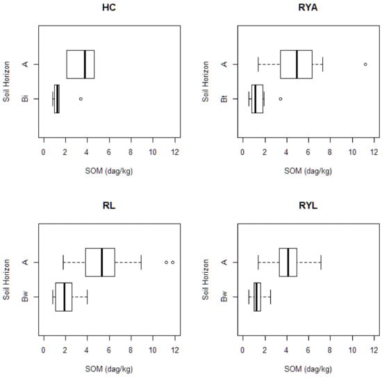
Figure 3.
Boxplots of soil organic matter (SOM) content by soil taxonomic class and soil horizon. RYL: Red-Yellow Latosol, RYA: Red-Yellow Argisol, RL: Red Latosol, HC: Haplic Cambisol.
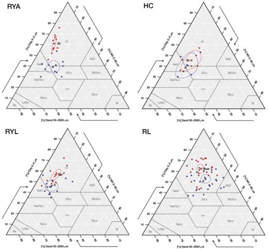
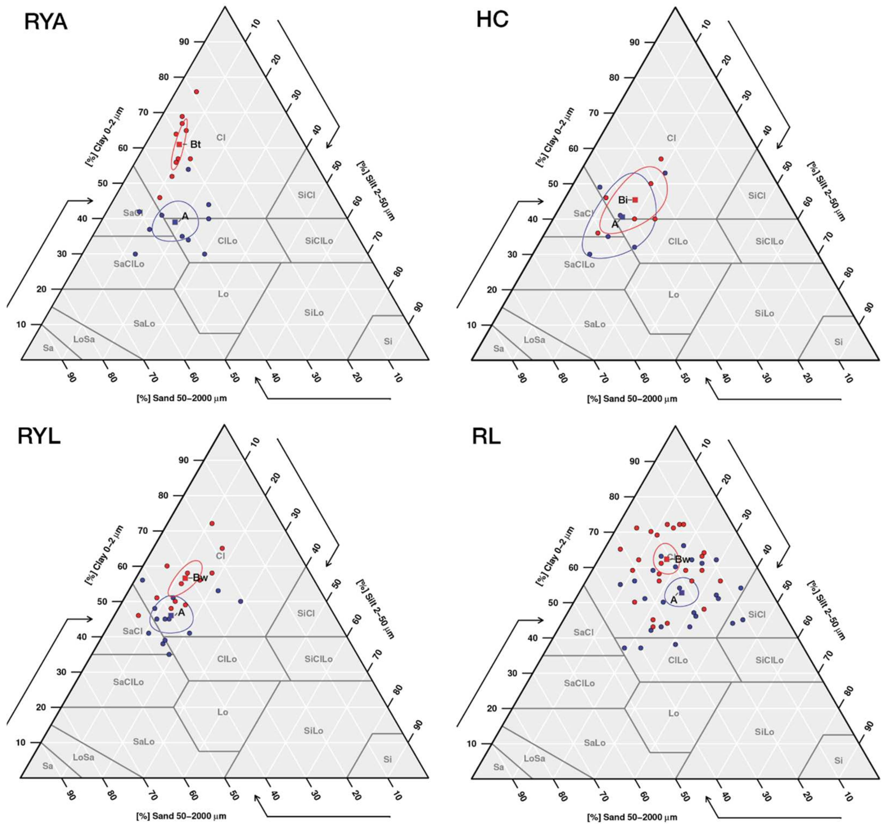
Figure 4.
Soil texture class distribution (dots) and center confidence regions (90% confidence) around centroids (squares) by soil horizon for each taxonomic class. Data points of A horizon in blue and B horizon in red. RYA: Red-Yellow Argisol, HC: Haplic Cambisol RYL: Red-Yellow Latosol, RL: Red Latosol. Cl: clay, SiCl: silty clay, SaCl: sandy clay, ClLo: clay loam, SiClLo: silty clay loam, SaClLo: sandy clay loam, Lo: loam, SiLo: silty loam, SaLo: sandy loam, Si: silt, LoSa: loamy sand, Sa: sand.
Although the origin of soil material can influence the soil formation, other factors and processes also play a role in determining soil characteristics. This can be demonstrated by looking at a chronosequence, which is a sequence of soils ordered by age, from younger to older. For example, in the chronosequence Haplic Cambisol → Red-Yellow Argisol → Red-Yellow Latosol and Red Latosol, the following physical and hydraulic characteristics were observed by Gonçalves et al. [47]: an increase in soil thickness, an increase in soil water storage capacity, a shift in B horizon structure from blocky to granular, an increase in permeability, a decrease in bulk density, and an increase in clay content. As for soil organic matter, the overall trend is that its concentration decreases with depth, with similar mean values among soils. However, some samples of Red-Yellow Argisol and Red Latosol have higher organic matter contents, as shown by the points in the boxplots.
3.2. Accuracy Assessment of DSM Predictive Models
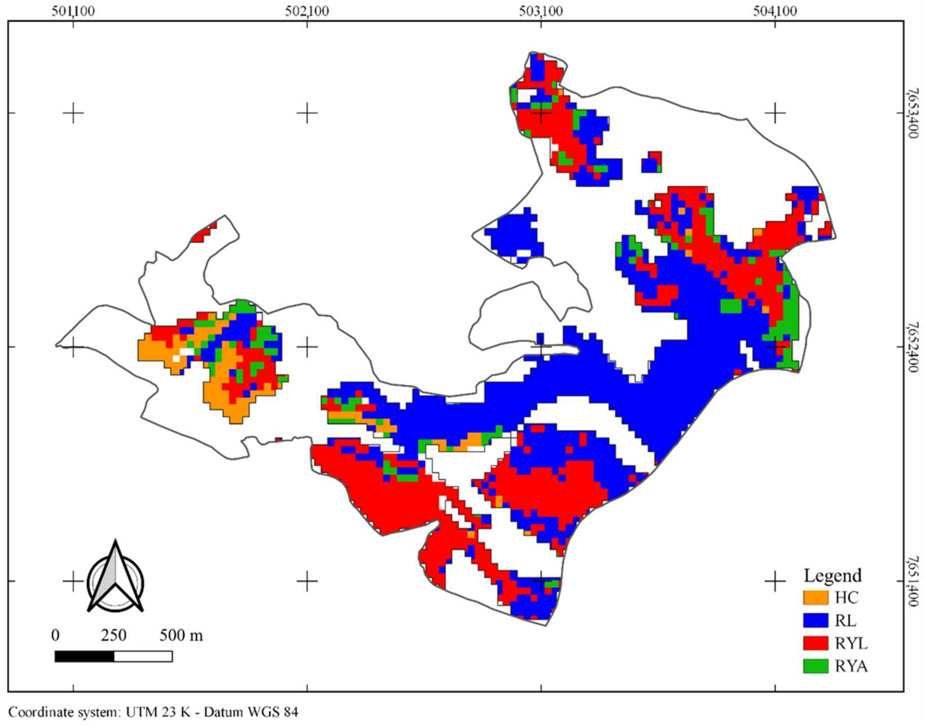
DSM predictive model presented a median global accuracy of 61.1% and a kappa value of 0.43, considered a fair level of agreement [48]. The error rate appeared to be proportional to the occurrence frequency of the analyzed soil classes. The dominant soil classes, such as Red Latosol (12.1%) and Red-Yellow Latosol (25.2%), had a lower error rate compared to the less frequent classes, such as Red-Yellow Argisol (47.3%) and Haplic Cambisol (87.3%). Figure 5 shows the soil map with only the pasture vegetation cover (164.74 ha) and the spatial distribution of the analyzed soils. The geographical distribution showed a predominance of Red Latosol (83.95 ha, representing 50.96% of the area), followed by Red-Yellow Latosol (58.55 ha, 35.54%), Red-Yellow Argisol (12.16 ha, 7.38%), and Haplic Cambisol (10.09 ha, 6.12%).

Figure 5.
Digital soil map under pasture cover at Federal University of Lavras, Minas Gerais state, Brazil. RYL: Red-Yellow Latosol, RYA: Red-Yellow Argisol, RL: Red Latosol, HC: Haplic Cambisol. Blank areas within the perimeter of the study area are vegetation types dissimilar to pasture.
3.3. Covariates Importance for DSM
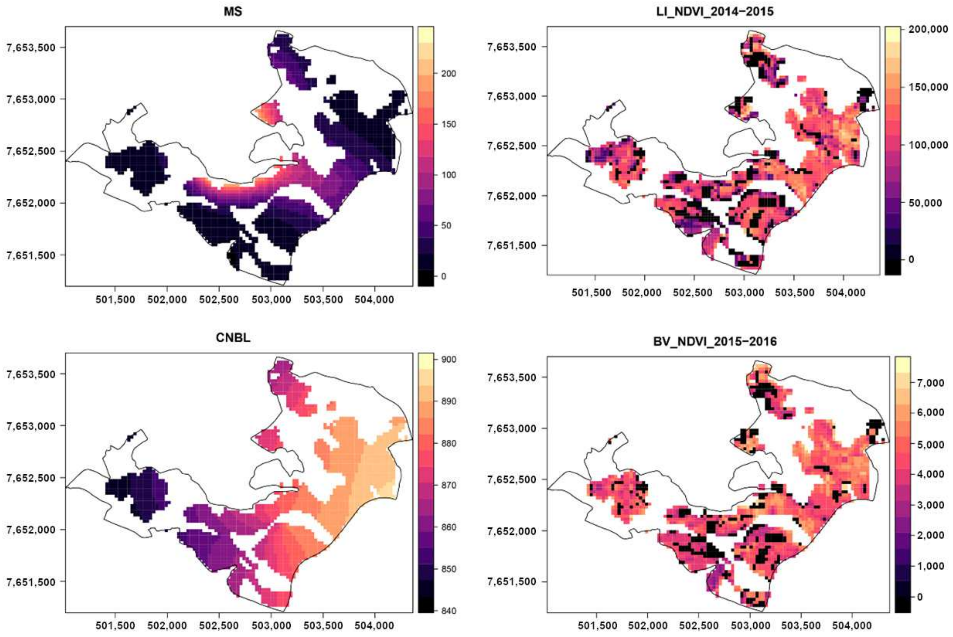
The results of the DSM evaluation of environmental covariates are displayed in Figure 6, showing the variable importance rank. The maps of the most important environmental covariates can be found in Figure 7. The LSP metrics, notably LI—NDVI and the base NDVI value of the seasons 2014–2015 and 2015–2016, were found to be as important as the covariates that depict parent material (magnetic susceptibility) and topography (CNBL). LI—NDVI is calculated by integrating the function spanning from the beginning to the end of each season using an asymmetric Gaussian function [30] and has been successfully associated with seasonal vegetation productivity [6,17,49]. The base level, which is defined as the averaged fitted minimum value of NDVI, has been reported as an efficient DSM covariate [21] and reflects the soil condition in which vegetation cycles are driven.
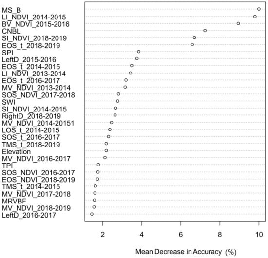
Figure 6.
Random forest variable importance of the covariates assessed for the digital soil map. MS_B: Magnetic susceptibility of B horizons, CNBL: channel network base level, SPI: stream power index, SWI: saga wetness index, TPI: topographic position index, MRVBF: multiresolution valley bottom flatness, SOS_t: time for the start of the season, EOS_t: time for the end of the season, LOS_t: length of the season, BV_NDVI: base level value, TMS_t: time for the middle of the season, MV_NDVI: maximum value for the fitted function during the season, Amp_NDVI: seasonal amplitude, LeftD: rate of increase at the beginning of the season (left derivative), RightD: rate of decrease at the end of the season (absolute value of right derivative), LI_NDVI: large seasonal integral, SI_NDVI: small seasonal integral, SOS_NDVI: value for the start of the season, EOS_NDVI: value for the end of the season.

Figure 7.
Random forest most important covariate maps: MS: Magnetic susceptibility of B horizons, CNBL: channel network base level, LI_NDVI: large seasonal integral, BV_NDVI: base level value. Black spots in LI and BV maps (below zero values) indicate insufficient data to fit a seasonal function.
3.4. Relationships between Rainfall and Vegetation Greenness for Each Soil Type
A correlation analysis was performed using Spearman’s rank correlation to investigate the relationship between median LI—NDVI values (which were identified as the most important LSP metric by random forest) and the accumulated seasonal rainfall. The analysis revealed that the soil type with the strongest correlation was RL, with a correlation coefficient of 0.7 and a p-value of less than 0.05 (Table 1). This suggests that there is a strong relationship between the pasture greenness over RL soil and the seasonal rainfall.

Table 1.
Spearman’s rank correlation (Rho) between seasonal rainfall and large integrated NDVI for each soil class.
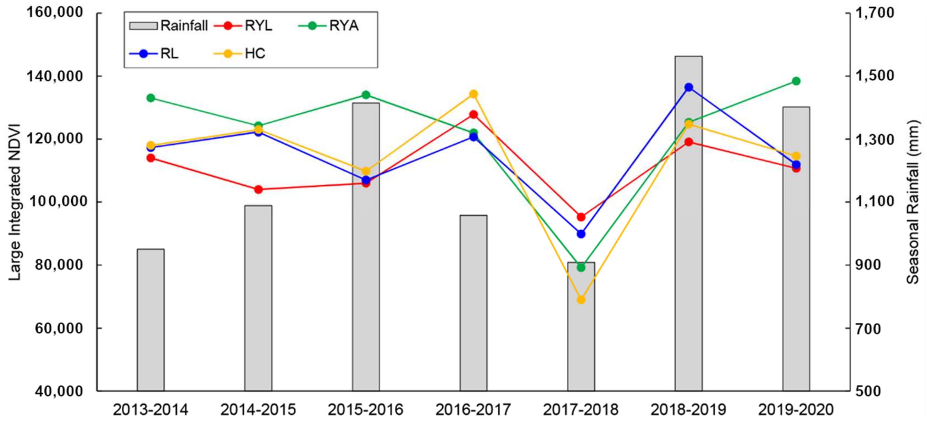
Figure 8 presents the complete time series of vegetation greenness based on the large integrated NDVI for each soil class. The vegetation response seems to depend on the accumulated rainfall in the previous season; a yearly scale can also be observed. It was observed that dissimilar median large integrated NDVI values responses to rainfall seasonality were present among all soil types, which reinforces the potential of such information as an environmental covariate in contrasting soils.

Figure 8.
Rainfall seasonality (grey bars) and its relation with large integrated NDVI (lines) for each soil taxonomic class. RYL: Red-Yellow Latosol, RYA: Red-Yellow Argisol, RL: Red Latosol, HC: Haplic Cambisol.
The Red-Yellow Argisol soil type presented higher values of large integrated NDVI in the seasons of 2013–2014, 2015–2016, and 2019–2020. This fact is thought to be related to increasing clay content in the B horizon and the blocky structure due to the pedogenetic process (illuvial clay accumulation). This fact along with higher SOM might increase the water-holding capacity even during dry seasons.
It is noteworthy that the Haplic Cambisols, the youngest and shallowest soil, exhibited low stability concerning vegetation responses. It reached the highest values of large integrated NDVI in the season 2016–2017 due to rainfall accumulation in the previous season and the lowest values in the next driest season (2017–2018), despite having high topsoil SOM content, which would increase the water-holding capacity of the soil.
The Red Latosol was the soil type more correlated with rainfall seasonality despite having high clay content. Latosols with oxidic mineralogy present a granular structure in the B horizon [46], and this structure is responsible for quite contrasting soil porous populations influencing plant water availability: macropores between aggregates and micropores within aggregates [50]. Water is held strongly in micropores, decreasing water availability for plants. Conversely, gravity readily removes water from macropores. Red Latosol has very high clay content, but Sans [51] noted that the unsaturated hydraulic conductivity decreases sharply within about two weeks of water saturation.
Thus, plant water availability was conditioned by soil class and reached its maximum expression during the period of 2017–2018 when decreasing water input produced the expected theoretical pattern. This fact was also verified by Méndez-Barroso et al. [52].
Previous research utilizing the integrated NDVI metric as a measure of seasonal productivity has revealed a correlation between soil moisture, clay content, and natural fertility [49,53]. As noted by Araya et al. [6], vegetation productivity is directly proportional to rainfall until it reaches a saturation point. This pattern is illustrated in Figure 8, which highlights similar processes, particularly for the RL soil type.
4. Discussion
4.1. Soil Control on the Response of Vegetation Greenness to Rainfall
Previous studies have confirmed that temporal variability of vegetation greenness is an effective covariate for digital soil mapping. Dematte et al. [15] found that analyzing the seasonal differences of NDVI can capture the influence of soil types on vegetation greenness, as different soil types reflect varying water dynamics in depth. Maynard and Levi [16] also verified that soil acts as the primary link between vegetation and climate feedback, further supporting the use of vegetation temporal variability as a DSM covariate. However, these studies did not explicitly consider the temporal dimension of vegetation in a phenological sense. Our research addresses this gap by analyzing the performance of time-synthetic images of NDVI phenological metrics and their relationship with seasonal rainfall as conditioned by soil types.
4.2. Suitability of LSP Data for DSM
Our study found that phenological synthetic imagery used as a DSM environmental covariate was just as important as parent material and relief proxies. This means that LSP imagery has great potential for use in DSM. However, it is important to note that the NDVI temporal signal may not accurately reflect the effects of water availability itself, as soil fertility and pollution can also impact the interaction between soil type and vegetation greenness. This can modify the time-spectral signature [15,54], thus affecting the results. Additionally, this fact might be one of the main sources of unexplained variability in the accuracy assessment. Therefore, future research should focus on functional signal filtering to identify stronger temporal signatures. These might be affected by biological indicators such as intraspecific or interspecific competition or genotypic diversity. Since this study was performed only in soils under pasture, the extension of this manuscript’s findings might be limited by biological indicators such as intraspecific or interspecific competition or genotypic diversity, since these factors also influence plant phenophases [55] (Menzel, 2002), which, in turn, might influence LSP.
5. Conclusions
This study investigated the effects of soil type on the response of vegetation greenness to rainfall in a seasonal context. Our research confirms that soil, in conjunction with rainfall seasonality, influences the temporal variability of vegetation greenness. The seasonal dynamics of rainfall act as a trigger for soil–plant interaction, causing the most responsive temporal signature when transitioning from a steady to a low-water input condition. While soil-forming factors such as parent material and topography are essential for soil classification and mapping, LSP metrics related to the availability of seasonal water to plants, large integrated NDVI, and the NDVI base level are also significant, particularly for the Red Latosol (Ferralsol). The map production process supports the use of vegetation seasonal metrics derived from remote sensing, along with other soil-forming factors, as a reliable source of information for the production of digital soil maps.
Author Contributions
Conceptualization, F.A.P.A., M.D.d.M., Soil survey and sample collection, M.D.d.M., N.C., Data analysis, F.A.P.A., M.D.d.M., F.W.A.J., Project management, M.L.N.S., N.C. Original draft, F.A.P.A., M.D.d.M., J.C.A., M.L.N.S. All authors have read and agreed to the published version of the manuscript.
Funding
This research was funded by the Coordenação de Aperfeiçoamento de Pessoal de Nível Superior—Brazil (CAPES)—Finance Code 001, Conselho Nacional de Desenvolvimento Científico e Tecnológico (CNPq), process: 307950/2021-2, and Fundação de Amparo à Pesquisa de Minas Gerais (FAPEMIG), process: APQ 00802-18.
Data Availability Statement
The data are available upon specific request to the authors.
Conflicts of Interest
The authors declare no conflicts of interest.
References
- McBratney, A.B.; Mendonça-Santos, M.L.; Minasny, B. On Digital Soil Mapping. Geoderma 2003, 117, 3–52. [Google Scholar] [CrossRef]
- Ma, Y.; Minasny, B.; Malone, B.P.; Mcbratney, A.B. Pedology and digital soil mapping (DSM). Eur. J. Soil Sci. 2019, 70, 216–235. [Google Scholar] [CrossRef]
- Wadoux, A.-C.; SamuelRosa, A.; Poggio, L.; Mulder, V.L. A note on knowledge discovery and machine learning in digital soil mapping. Eur. J. Soil Sci. 2020, 71, 133–136. [Google Scholar] [CrossRef]
- Coelho, F.F.; Giasson, E.; Campos, A.R.; Tiecher, T.; Costa, J.J.F.; Coblinski, J.A. Digital soil class mapping in Brazil: A systematic review. Sci. Agric. 2020, 78, e20190227. [Google Scholar] [CrossRef]
- Soil Science Division Staff. Soil Survey Manual, 4th ed.; Handbook No. 18.; U.S. Department of Agriculture, U.S. Government Printing Office: Washington, DC, USA, 2017.
- Araya, S.; Lyle, G.; Lewis, M.; Ostendorf, B. Phenologic metrics derived from MODIS NDVI as indicators for Plant Available Water-holding Capacity. Ecol. Indic. 2016, 60, 1263–1272. [Google Scholar] [CrossRef]
- Fujii, K.; Shibata, M.; Kitajima, K.; Ichie, T.; Kitayama, K.; Turner, B.L. Plant–soil interactions maintain biodiversity and functions of tropical forest ecosystems. Ecol. Res. 2018, 33, 149–160. [Google Scholar] [CrossRef]
- Berry, S.L.; Mackey, B. On modelling the relationship between vegetation greenness and water balance and land use change. Sci. Rep. 2018, 8, 9066. [Google Scholar] [CrossRef] [PubMed]
- IBGE. Manual técnico de pedologia. In Coordenação de Recursos Naturais e Estudos Ambientais, 3rd ed.; IBGE: Rio de Janeiro, Brazil, 2007; 430p. [Google Scholar]
- Helman, D. Land surface phenology: What do we really ‘see’ from space? Sci. Total Environ. 2018, 618, 665–673. [Google Scholar] [CrossRef] [PubMed]
- Mulder, V.L.; de Bruin, S.; Schaepman, M.E.; Mayr, T.R. The use of remote sensing in soil and terrain mapping—A review. Geoderma 2011, 162, 1–19. [Google Scholar] [CrossRef]
- Rouse, J.W.; Haas, R.J.; Schell, J.A.; Deering, D.W. Monitoring vegetation systems in the Great Plains with ERTS. In NASA SP-351, Third ERTS-1 Symposium; Texas A&M University: College Station, TX, USA, 1974; pp. 309–317. [Google Scholar]
- Padarian, J.; Minasny, B.; McBratney, A.B. Using Google’s cloud-based platform for digital soil mapping. Comput. Geosci. 2015, 83, 80–88. [Google Scholar] [CrossRef]
- Dwyer, J.L.; Roy, D.P.; Sauer, B.; Jenkerson, C.B.; Zhang, H.K.; Lymburner, L. Analysis ready data: Enabling analysis of the landsat archive. Remote Sens. 2018, 10, 1363. [Google Scholar] [CrossRef]
- Demattê, J.A.M.; Sayão, V.M.; Rizzo, R.; Fongaro, C.T. Soil class and attribute dynamics and their relationship with natural vegetation based on satellite remote sensing. Geoderma 2017, 302, 39–51. [Google Scholar] [CrossRef]
- Maynard, J.J.; Levi, M.R. Hyper-temporal remote sensing for digital soil mapping: Characterizing soil-vegetation response to climatic variability. Geoderma 2017, 285, 94–109. [Google Scholar] [CrossRef]
- Li, Z.; Huffman, T.; Zhang, A.; Zhou, F.; McConkey, B. Spatially locating soil classes within complex soil polygons—Mapping soil capability for agriculture in Saskatchewan Canada. Agric. Ecosyst. Environ. 2012, 152, 59–67. [Google Scholar] [CrossRef]
- Caparros-Santiago, J.A.; Rodriguez-Galiano, V.; Dash, J. Land surface phenology as indicator of global terrestrial ecosystem dynamics: A systematic review. ISPRS J. Photogramm. Remote Sens. 2021, 171, 330–347. [Google Scholar] [CrossRef]
- Wolkovich, E.M.; Cook, B.I.; Allen, J.M.; Crimmins, T.M.; Betancourt, J.L.; Travers, S.E.; Pau, S.; Regetz, J.; Davies, T.J.; Kraft, N.J.; et al. Warming experiments underpredict plant phenological responses to climate change. Nature 2012, 485, 494–497. [Google Scholar] [CrossRef] [PubMed]
- Jönsson, P.; Eklundh, L. TIMESAT—A program for analyzing time-series of satellite sensor data. Comput. Geosci. 2004, 30, 833–845. [Google Scholar] [CrossRef]
- Yang, L.; He, X.; Shen, F.; Zhou, C.; Zhu, A.-X.; Gao, B.; Chen, Z.; Li, M. Improving prediction of soil organic carbon content in croplands using phenological parameters extracted from NDVI time series data. Soil Tillage Res. 2020, 196, 104465. [Google Scholar] [CrossRef]
- Fathololoumi, S.; Vaezi, A.R.; Alavipanah, S.K.; Ghorbani, A.; Saurette, D.; Biswas, A. Improved Digital Soil Mapping with Multitemporal Remotely Sensed Satellite Data Fusion: A Case Study in Iran. Sci. Total Environ. 2018, 721, 137703. [Google Scholar] [CrossRef]
- Curi, N.; Silva, S.H.G.; Poggere, G.C.; Menezes, M.D. Mapeamento de Solos e Magnetismo no Campus da UFLA Como Traçadores Ambientais; UFLA: Lavras, MG, Brazil, 2017; ISBN 978-85-8127-052-4. [Google Scholar]
- Santos, H.G.d.; Jacomine, P.K.T.; Anjos, L.H.C.d.; Oliveira, V.A.d.; Lumbreras, J.F.; Coelho, M.R.; Almeida, J.A.d.; Araujo Filho, J.C.d.; Oliveira, J.B.d.; Cunha, T.J.F. Brazilian Soil Classification System; Embrapa: Brasilia, DF, Brasil, 2018; Available online: https://www.embrapa.br/busca-de-publicacoes/-/publicacao/1094001/brazilian-soil-classification-system (accessed on 18 August 2020).
- Embrapa. Manual de Análises Químicas de Solos, Plantas e Fertilizantes, 1st ed.; Solos, E., Ed.; Embrapa: Rio de Janeiro, Brazil, 1999. [Google Scholar]
- Alvares, C.A.; Stape, J.L.; Sentelhas, P.C.; Gonçalves, J.L.M.; Sparovek, G. Köppen’s Climate Classification Map for Brazil. Meteorol. Z. 2013, 6, 711–728. [Google Scholar] [CrossRef]
- Souza, C.M.; Shimbo, J.Z.; Rosa, M.R.; Parente, L.L.; Alencar, A.A.; Rudorff, B.F.T.; Hasenack, H.; Matsumoto, M.; Ferreira, L.G.; Souza-Filho, P.W.M.; et al. Reconstructing Three Decades of Land Use and Land Cover Changes in Brazilian Biomes with Landsat Archive and Earth Engine. Remote Sens. 2020, 12, 735. [Google Scholar] [CrossRef]
- Hijmans, R.J. Raster: Geographic Data Analysis and Modeling. 2020. Available online: https://cran.r-project.org/package=raster (accessed on 5 April 2020).
- R-Core-Team. R: A Language and Environment for Statistical Computing; R-Core-Team: Vienna, Austria, 2019; Available online: https://www.R-project.org (accessed on 10 April 2020).
- Eklundh, L.; Jönsson, P. Timesat—Software Manual; Lund and Malmö University: Lund, Sweden, 2017; Available online: http://www.nateko.lu.se/TIMESAT/ (accessed on 5 January 2020).
- Hird, J.N.; McDermid, G.J. Noise reduction of NDVI time series: An empirical comparison of selected techniques. Remote Sens. Environ. 2009, 113, 248–258. [Google Scholar] [CrossRef]
- Conrad, O.; Bechtel, B.; Bock, M.; Dietrich, H.; Fischer, E.; Gerlitz, L.; Wehberg, J.; Wichmann, V.; Boehner, J. System for Automated Geoscientific Analyses (SAGA) v. 2.1.4. Geosci. Model Dev. 2015, 8, 1991–2007. [Google Scholar] [CrossRef]
- Zheng, X.; Xiong, H.; Yue, L.; Gong, J. An improved ANUDEM method combining topographic correction and DEM interpolation. Geocarto Int. 2016, 31, 492–505. [Google Scholar] [CrossRef]
- Silva, S.; Poggere, G.; Menezes, M.; Carvalho, G.; Guilherme, L.; Curi, N. Proximal sensing and digital terrain models applied to digital soil mapping and modeling of Brazilian Latosols (Oxisols). Remote Sens. 2016, 8, 614. [Google Scholar] [CrossRef]
- Gee, G.W.; Bauder, J.W. Particle-Size Analysis. In Methods of Soil Analysis; Klute, A., Ed.; American Society of Agronomy: Madison, WI, USA, 1986; pp. 383–412. [Google Scholar]
- Breiman, L. Random Forests. Machine Learning 2001, 45, 5–32. [Google Scholar] [CrossRef]
- Liaw, A.; Wiener, M. Classification and regression by randomForest. R News 2002, 2, 18–22. [Google Scholar] [CrossRef]
- Hengl, T.; Nussbaum, M.; Wright, M.N.; Heuvelink, G.B.M.; Gräler, B. Random forest as a generic framework for predictive modeling of spatial and spatio-temporal variables. PeerJ 2018, 6, e5518. [Google Scholar] [CrossRef] [PubMed]
- Heung, B.; Ho, H.C.; Zhang, J.; Knudby, A.; Bulmer, C.E.; Schmidt, M.G. An overview and comparison of machine-learning techniques for classification purposes in digital soil mapping. Geoderma 2016, 265, 62–77. [Google Scholar] [CrossRef]
- Silva, B.P.C.; Silva, M.L.N.; Avalos, F.A.P.; de Menezes, M.D.; Curi, N. Digital soil mapping including additional point sampling in Posses ecosystem services pilot watershed, southeastern Brazil. Sci. Rep. 2019, 9, 13763. [Google Scholar] [CrossRef] [PubMed]
- Khaledian, Y.; Miller, B.A. Selecting appropriate machine learning methods for digital soil mapping. Appl. Math. Model. 2020, 81, 401–418. [Google Scholar] [CrossRef]
- Soil-Survey-Staff. Keys to Soil Taxonomy, 12th ed.; USDA-Natural Resources Conservation Service: Washington, DC, USA, 2014.
- IUSS Working Group WRB. World Reference Base for Soil Resources 2014, Update 2015 International Soil Classification System for Naming Soils and Creating Legends for Soil Maps; World Soil Resources Reports No. 106; FAO: Rome, Italy, 2015; Available online: https://www.fao.org/3/i3794en/I3794en.pdf (accessed on 15 January 2020).
- Congalton, R.G. Accuracy Assessment and Validation of Remotely Sensed and Other Spatial Information. Int. J. Wildland Fire 2001, 10, 321–328. [Google Scholar] [CrossRef]
- Wadoux, A.M.-C.; Molnar, C. Beyond prediction: Methods for interpreting complex models of soil variation. Geoderma 2021, 422, 115953. [Google Scholar] [CrossRef]
- Resende, M.; Curi, N.; Rezende, S.D.; Silva, S.H.G. Da Rocha ao Solo: Enfoque Ambiental; UFLA: Lavras, Brazil, 2019. [Google Scholar]
- Gonçalves, M.G.M.; Brant, L.A.C.; Mota, R.V.D.; Peregrino, I.; Souza, C.R.D.; Regina, M.D.A.; Fruett, T.; Inda, A.V.; Curi, N.; Menezes, M.D.D. Soil and climate effects on winter wine produced under the tropical environmental conditions of southeastern Brazil. OENO One 2022, 56, 63–79. [Google Scholar] [CrossRef]
- Landis, J.R.; Koch, G.G. The Measurement of Observer Agreement for Categorical Data. Biometrics 1977, 33, 159–174. [Google Scholar] [CrossRef] [PubMed]
- Nicholson, S.E.; Farrar, T.J. The influence of soil type on the relationships between NDVI, rainfall and soil moisture in semiarid Botswana. I. NDVI response to rainfall. Remote Sens. Environ. 1994, 50, 107–120. [Google Scholar] [CrossRef]
- Carducci, C.E.; de Oliveira, G.C.; Severiano, E.d.C.; Zeviani, W.M. Modelagem da curva de retenção de água de Latossolos utilizando a Equação Duplo Van Genuchten. Rev. Bras. Ciênc. Solo 2011, 35, 77–86. [Google Scholar] [CrossRef]
- Sans, L.M.A. Estimativa do Regime de Umidade Pelo Método de Newhall, de um Latossolo Vermelho-Escuro Álico da Região de Sete Lagoas, MG. Ph.D. Thesis, Universidade Federal de Viçosa, Viçosa, Brazil, 1986; 190p. [Google Scholar]
- Méndez-Barroso, L.A.; Vivoni, E.R.; Watts, C.J.; Rodríguez, J.C. Seasonal and interannual relations between precipitation, surface soil moisture and vegetation dynamics in the North American monsoon region. J. Hydrol. 2009, 377, 59–70. [Google Scholar] [CrossRef]
- Farrar, T.J.; Nicholson, S.E.; Lare, A.R. The influence of soil type on the relationships between NDVI, rainfall, and soil moisture in semiarid Botswana. II. NDVI response to soil moisture. Remote Sens. Environ. 1994, 50, 121–133. [Google Scholar] [CrossRef]
- Gholizadeh, A.; Kopačková, V. Detecting vegetation stress as a soil contamination proxy: A review of optical proximal and remote sensing techniques. Int. J. Environ. Sci. Technol. 2019, 16, 2511–2524. [Google Scholar] [CrossRef]
- Menzel, A. Phenology: Its importance to the global change community. Clim. Change 2002, 54, 379. [Google Scholar] [CrossRef]


Disclaimer/Publisher’s Note: The statements, opinions and data contained in all publications are solely those of the individual author(s) and contributor(s) and not of MDPI and/or the editor(s). MDPI and/or the editor(s) disclaim responsibility for any injury to people or property resulting from any ideas, methods, instructions or products referred to in the content. |
© 2024 by the authors. Licensee MDPI, Basel, Switzerland. This article is an open access article distributed under the terms and conditions of the Creative Commons Attribution (CC BY) license (https://creativecommons.org/licenses/by/4.0/).