Monitoring of Woody Biomass Quality in Italy over a Five-Year Period to Support Sustainability

Abstract

Biomass continues to play a key role as an alternative to fossil fuels. Woody biomass produces lower greenhouse gas emissions than fossil fuels. However, in order to consider biomass as ‘green energy’, a number of factors should be taken into account, including the characterization of the quality of the resource. Therefore, monitoring quality parameters, such as moisture, ash, N content, is essential to assess the sustainability of biomass for energy production. This paper presents the results of laboratory analyses performed on wood chip samples from four Italian regions over a five-year period (2019–2023). In particular, all quality parameters defined by ISO 17225-9 for industrial wood chips were assessed. Data were analyzed using descriptive, parametric, non-parametric statistics, and multivariate analysis. An interest in quality monitoring has been observed, indicated by an increase in the number of samples received from suppliers and an enhancement in the average values of quality parameters. Moreover, an overall decrease in moisture and N content has been observed, while ash content and heating value have undergone non-linear variations. Statistically significant quality differences between samples from different regions may be the result of different practices, such as outdoor or indoor storage, climate differences, different biomass growth conditions.

1. Introduction

According to the latest report from the European Parliament’s 2023 Committee [1], solid biomass continues to play a key role as an alternative to fossil fuels. While a variety of biomasses are used, such as agricultural residues and prunings from vineyards and olive trees [2], forestry (woody) biomass is the most widely used by Member States [1]. Eurostat data from 2020 indicates that approximately 32% of Italy’s territory is forested, translating to an estimated 1,424,400 thousand cubic meters of available wood [3]. Moreover, this forested area has been steadily increasing, growing by 26% between 1990 and 2020 [4].

Despite the significant availability of woody biomass in Italy, its potential is not fully exploited in some regions, particularly in northern Italy [5]. Similar underutilization is observed in other parts of the country, excluding a few areas in central and southern Italy [6]. Contributing factors to the under-exploitation include challenging land morphology, which makes wood resources difficult to access, and the fragmentation of forest property [7,8]. However, recent European incentives and policies [9] have spurred the development of biomass-fueled thermal power plants [10,11]. Furthermore, countries outside Europe are also embracing biomass for sustainable energy production [12,13].

Woody biomasses emit fewer greenhouse gases (GHGs) compared to fossil fuels [14,15]. However, to consider biomass as ‘green energy’, several factors must be considered, including supply chain sustainability [16,17] and resources’ quality characterization [16,18], which directly impact energy capacity and combustion efficiency [19,20]. Indeed, moisture content significantly affects combustion efficiency, with higher moisture levels increasing carbon monoxide (CO) emissions and thermal load [19,21]. Similarly, higher nitrogen content in biomass leads to increased nitrogen oxide (NOx) emissions [22].

Biomasses’ quality also influences its economic value due to contracts between power plants and suppliers being based on parameters such as calorific value and consequently on the moisture content of the supplied biofuel. Therefore, monitoring these quality parameters is essential for assessing the sustainability of biomass for energy production [23,24].

In the context of ensuring biomasses’ quality, ISO standards come into play. Specifically, the ISO 17225-1 [25] standard outlines the specifications and classification of solid biofuels, while ISO 17225-9 [26] specifically addresses wood chips for industrial use, identifying four quality Classes ranging from I1 to I4. For example, the moisture content for Class I1 must be ≤ 45% of the sample weight, whereas Class I4 allows values ≤ 60%.

Since 2013, the Biomass Laboratory at the Polytechnic of Marche has been dedicated to the qualitative analysis of woody and herbaceous biomasses, such as wood chips, pellets, sorghum, and corn. Over time, an increasing number of operators in the sector, such as suppliers and power plants, have come to rely on the Biomass Laboratory for the qualitative monitoring of their materials. This has led to the acquisition of a significant amount of data. A critical analysis of the overall quality of biomasses in Italy over a five-year period is therefore presented, focusing specifically on wood chips, highlighting a temporal and geographical difference between samples. To the best of the authors’ knowledge, this is the first study in Italy to assess biomass quality using an extensive database of laboratory analyses, rather than relying solely on literature data. As a result, the data presented here provide a robust foundation for future research and discussions on woody biomass for energy production.

2. Materials and Methods

This study presents the results of qualitative analyses performed on wood chip samples from four Italian regions over a five-year period (2019–2023). The samples were received from different suppliers and analyzed according to their specific requirements. The required analyses, performed according to standard methodology, included the assessment of moisture content (MC, ISO 18134-2 [27]), ash content (ASH, ISO 18122 [28]), heating value (HV, ISO 18125 [29]), organic chemical composition (C, H, N–ISO 16948 [30]), and chlorine and sulfur content (Cl, S–ISO 16994 [31]). The total number of samples analyzed from each region was as follows: 5356 from Emilia-Romagna (central-northern Italy, with subcontinental and sublittoral climate), 1642 from Calabria (southern Italy, mostly characterized by warm temperate climate), 440 from Sicilia (isle in southern Italy, with warm temperate-sublittoral climate and some subcontinental areas), and 280 from Sardegna (isle in western Italy, with predominantly warm temperate and sublittoral climate).

The data obtained from the qualitative analyses were then subjected to various statistical analyses, ranging from descriptive statistics, parametric, non-parametric statistics, and multivariate analysis. The data were compared with the limit values defined for quality Classes in ISO 17225-9 in order to assess whether the annual averages were compatible with the values defined in the standard, with the exception of net heating value (NHV), for which no limit values were defined. Lastly, in descriptive, parametric, and non-parametric statistics, oxygen (O) values (obtained from the measured values of C, H, N) were not taken into account.

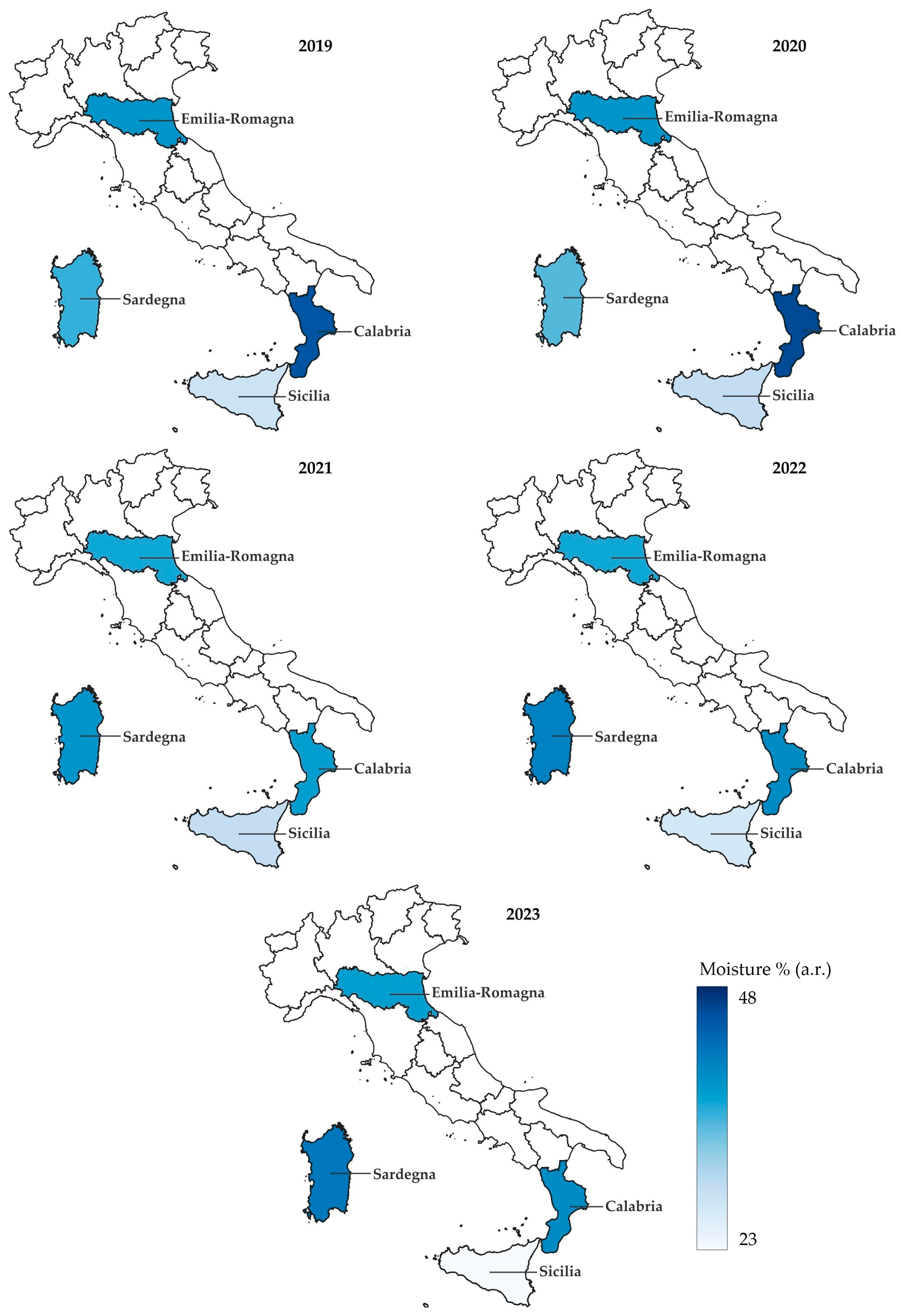
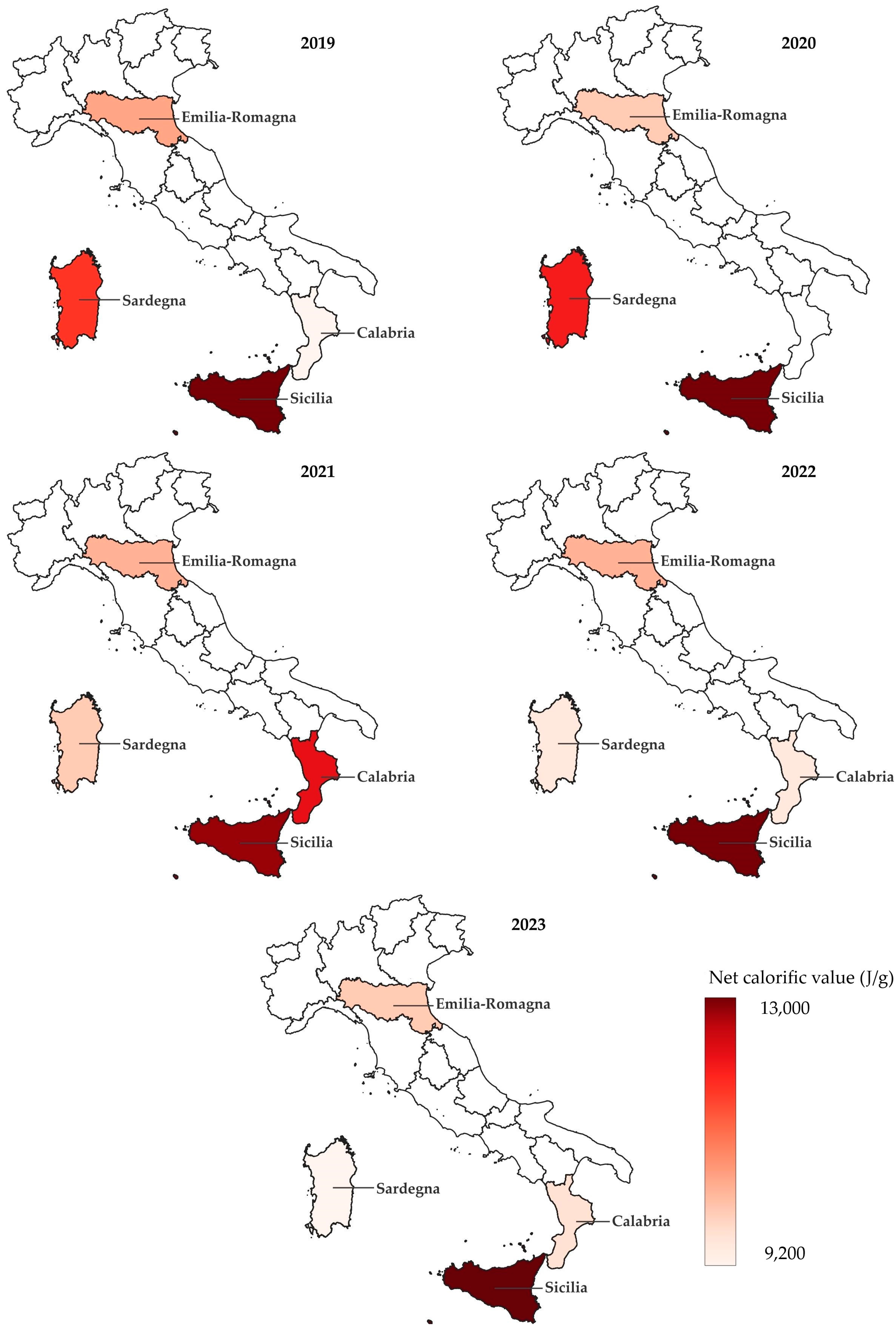
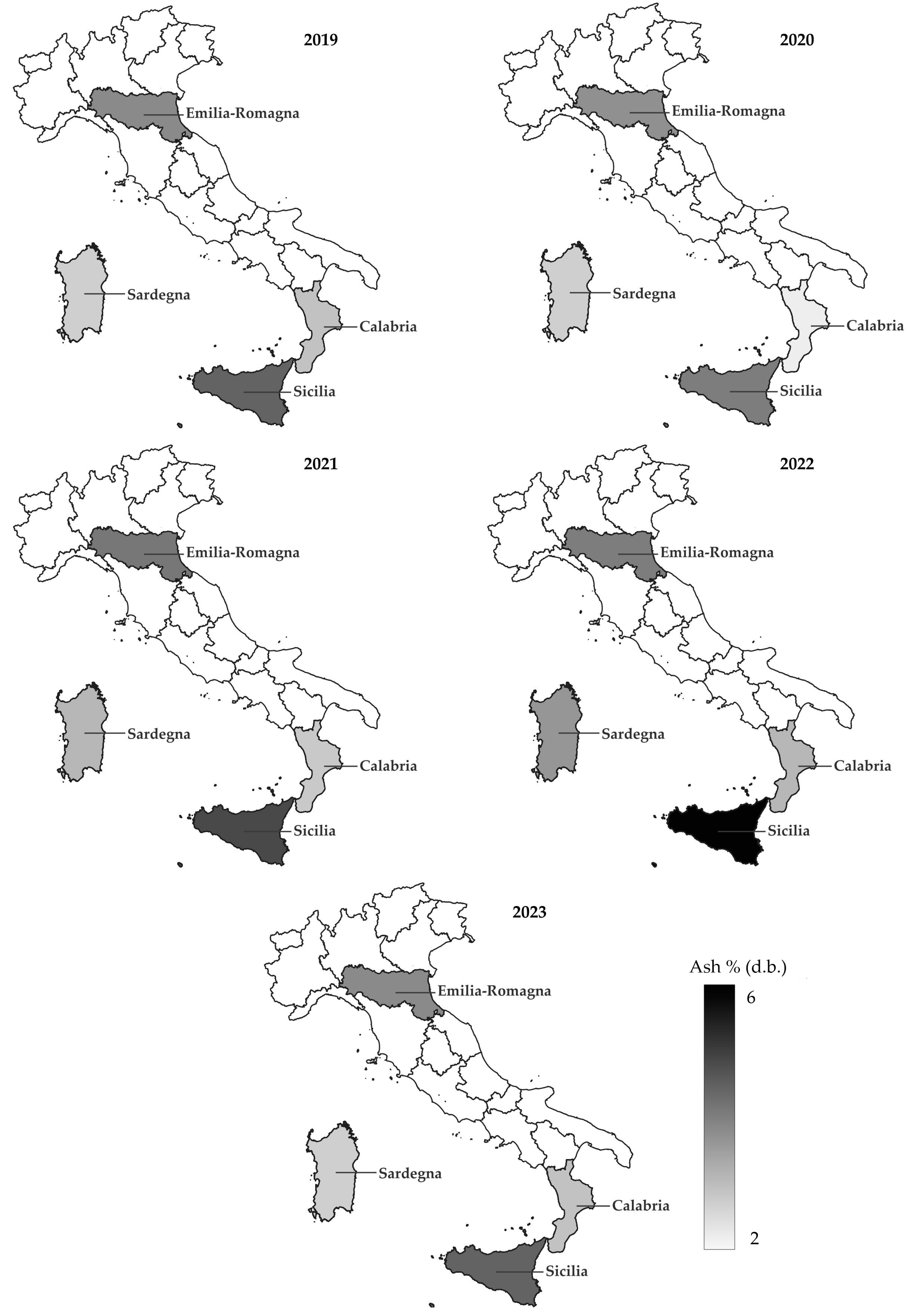
2.1. Descriptive Statistics and Quality Mapping

Firstly, descriptive statistics, such as mean, standard deviation (σ), median, and inter-quartile range (IQR), were used to process data from the samples obtained from the four regions over the five-year period. Analyses’ results were used to create thematic maps to support the visualization of trends in biomass quality over time. Thematic maps were produced using QGIS (version 3.34.7 LTR) for the most relevant qualitative parameters, specifically those in which biomass suppliers have the greatest interest and therefore demand for analysis. Therefore, the mapped parameters included MC, NHV, and N. Interpretation of the thematic maps, which provide information on the mean and median values of the displayed parameters, is facilitated by the use of colors that increase in saturation as the magnitude of the data displayed increases.

2.2. Parametric and Non-Parametric Statistics

For each considered region, the data obtained over the course of the five-year period were combined, resulting in four data sets that were subjected to advanced statistical analysis. The statistical analysis focused mainly on the data related to the main biomass quality parameters, namely MC, NHV, ASH, and N. Anderson–Darling normality tests (AD), quantile–quantile plots (Q-Q), and one-way analysis of variance (ANOVA) were carried out for each main parameter to assess whether the qualitative average differences between regions were statistically significant. Tukey’s HSD test was carried out to assess which region differed from the others. For non-normal data, Kruskal–Wallis (KW) was used to evaluate significant differences among regional medians, followed by Dunn’s Test (DT) to assess which pair of regions differed from the others.

To assess the strength of the evidence against the null hypothesis (p), both parametric and non-parametric analyses were performed with a significance level (α) of 0.05. Specifically, in AD, a p-value < α indicates a rejection of the assumption of normality, while for ANOVA and KW, a p-value < α, indicates a statistically significant difference among the datasets. Furthermore, the F statistic (F) in ANOVA and the H statistic (H) in the Kruskal–Wallis test were reported to highlight the magnitude of differences between datasets; larger values indicate greater differences. Lastly, where deemed useful for the interpretation of the data, the asymmetry of data distribution was also monitored by assessing data’s skewness.

The aforementioned analyses have been carried out with Python 3.11 and libraries such as Pandas [32], Scipy [33], Matplotlib [34], and Statsmodels [35].

2.3. Multivariate Analysis

Principal Component Analysis (PCA) has been carried out to extract and explore the statistical variance of datasets based on the main physical and chemical parameters. Thus, the original dataset has been converted into a new and reduced and simplified space created by the orthogonal components (Principal Components, or PCs) which explain the maximum variance of the dataset [36,37]. Considering the different scales of each parameter, PCA was performed after data normalization.

Two different approaches have been used to study the quality parameters, namely the variables:

(i) Spatial analysis (SA): Annual data from the four regions were combined to produce five matrices (one per year, containing data from the four regions), which were used to investigate the possibility of a spatial variation in biomass quality due to climatic influences.

(ii) Temporal analysis (TA): Regional data collected over the five years were combined into four matrices (one per region, containing data collected over the whole period for each region), which were used to examine the internal quality of the regions.

Despite the considerable amount of data collected, the dataset lacked comprehensive results for some samples due to the different requirements of each supplier. Therefore, the database used to develop the PCA was pre-processed to remove incomplete data. This allowed all the variables to be used correctly, thus creating a consistent scenario of the relationship between them. For this reason, Pearson’s analysis was also employed to assess the degree and type of correlation between the variables considered. Variables with r < ±0.4 were not considered.

The main results of interest from the PCA have been graphically presented in their corresponding biplot, which brings together the sample distribution (provided by the score plot) and the attributable influence of the variables (provided by the loading plot) to detect the nature and degree of their correlation [38]. Matlab R2021a (ver.9.10) software was used to perform the PCA analysis, using built-in scripts.

3. Results and Discussions

3.1. Descriptive, Parametric, and Non-Parametric Statistics

The results of the descriptive analyses, displayed in thematic maps in the final section of the paper, have been combined with the results of the parametric and non-parametric statistics, reporting the main outcomes of each investigated parameter.

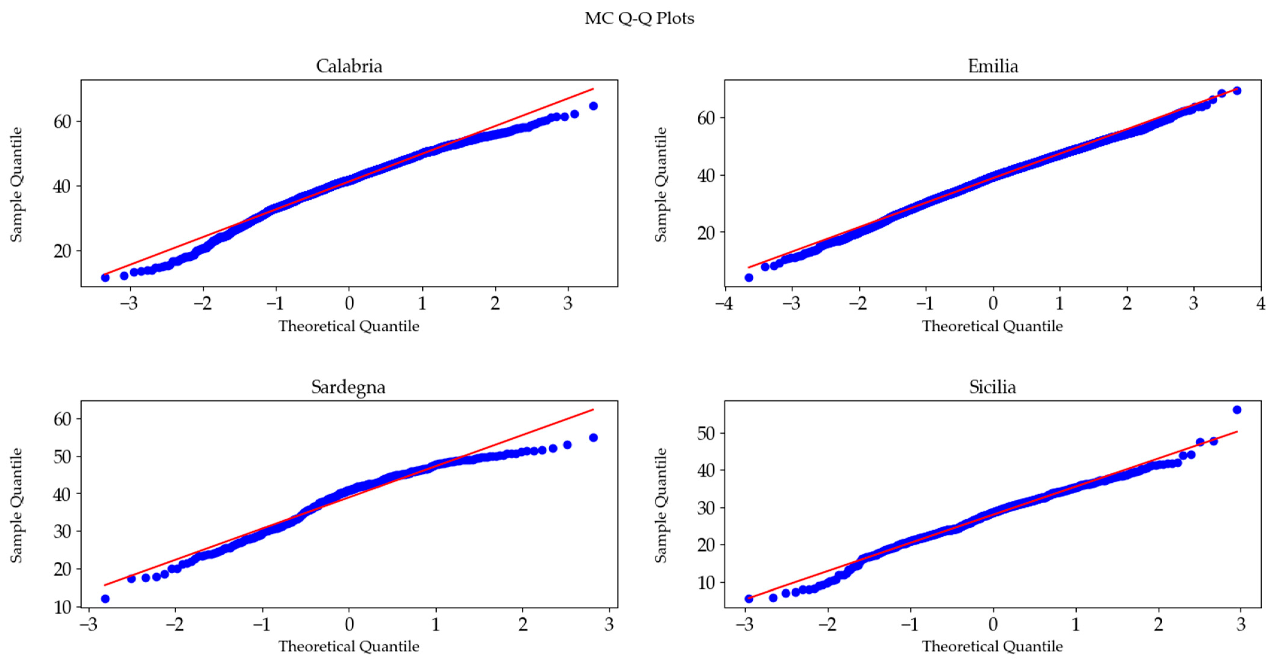
3.1.1. Moisture Content

During the five-year period, the number of MC analyses performed on samples from each region were 5111 from Emilia-Romagna, 1642 from Calabria, 280 from Sardegna, and 440 from Sicilia (

Table 1. Summary of MC data acquired during the 5-year period. Yearly mean values, as well as yearly quartiles (Q1, Q2, and Q3), are reported as a percentage of as-received mass.

	Moisture Content (% a.r.)
Region	Year	N. Samples	Mean	St. Dev.	Q1	Q2	Q3
EMILIA - ROMAGNA	2019	465	39.3	7.8	34.2	40.7	44.3
	2020	800	39.3	8.1	34.3	39.9	44.1
	2021	1143	37.8	8.3	34.4	40.3	45.2
	2022	1266	37.6	9.4	31.5	37.6	44.4
	2023	1437	38.3	8.3	32.7	38.6	44.2
	2019	123	45.3	7.6	41.8	45.9	49.4
	2020	91	46.5	7.5	41.6	47.5	52.2
CALABRIA	2021	212	38.1	10.6	31.9	40.5	45.6
	2022	622	40.7	7.7	36.1	41.2	45.9
	2023	594	41.0	8.5	35.5	41.2	47.3
	2019	72	36.8	7.3	30.8	38.2	42.4
	2020	48	35.7	8.9	30.1	36.6	42.6
SARDEGNA	2021	56	39.2	7.9	34.5	40.1	44.6
	2022	58	41.0	9.1	35.7	44.4	48.2
	2023	46	42.7	7.4	40.6	44.8	48.0
	2019	94	28.7	7.1	23.9	30.4	34.1
	2020	89	29.3	6.3	24.9	28.6	33.6
SICILIA	2021	98	29.6	8.0	22.7	30.3	36.2
	2022	91	27.3	7.7	23.3	28.0	31.6
	2023	68	23.5	7.1	19.0	23.1	28.6

). For the avoidance of any misunderstanding, the mean MC values are given in % followed by σ, while the relative annual variation between the mean MC is given in % without σ (i.e., a 10% increase in MC 40%, σ = 5.0, corresponds to an MC of 44%, σ = 5.0).

The number of samples received from Emilia-Romagna showed a steady increase throughout the study period, with the most significant increase occurring between 2019 and 2020 when the number of samples rose from 465 to 800. Overall, the number of samples analyzed increased by 209% between 2019 and 2023. The average annual MC values ranged between 37% and approximately 40% with positive and negative fluctuations during the entire period. Between 2020 and 2021, MC decreased from an average MC of 39.3% (σ = 8.1) to 37.8% (σ = 8.3) to finally increase to 38.3% (σ = 8.3) in 2023. Finally, greater variability in MC values from the region was suggested by the trend of the IQR over time, which tended to increase. Lastly, Emilia-Romagna’s samples presented eligible MC values to quality Class I1 (required MC ≤ 45%) for the entire period.

The number of samples analyzed from Calabria varied significantly over the years. After a decrease of 26% between 2019 and 2020, there was a remarkable increase of 193.4% between 2021 and 2022. Overall, the number of samples analyzed grew by 382% from 2019 to 2023, rising from 123 samples to 594. Similarly to the previous region, samples from Calabria have shown varying MC levels over time, consistently remaining higher than those from Emilia-Romagna. Notably, the average MC was particularly high in 2020, reaching 46.5% (σ = 7.5). However, there was a significant decrease in MC between 2019 and 2023, thus going from 45.3% (σ = 7.6) to 41% (σ = 8.5), juxtaposed by a 53.82% increase in IQR. Nevertheless, Calabria samples showed MC values falling into quality Class I1, with the exception of the first two years, which were characterized by values falling into Class I2 (≤50%).

Sardegna was the region from which the fewest samples were obtained, with 72 samples obtained in 2019, decreasing to 46 in 2023. While the first two years resulted in lower MC values than in Emilia-Romagna and Calabria, the following years were characterized by a steady increase, culminating in average MC values in 2023 of 42.7% (σ = 7.4), a percentage increase of 16% compared to 2019. Of further note, the IQR decreased by 36% between 2019–2023, indicating less variability in MC values over time. Moreover, Sardegna’s samples presented MC values fitting to quality Class I1 for the entire period.

Over time, the number of samples received from suppliers located in Sicilia has remained constant, with only one decrease of around 25% between 2022 and 2023, thus from 91 samples to 68. As well as having the lowest MC values compared to the other regions, the annual values decreased by 18% over the whole period, starting from an MC of 28.7% (σ = 7.1) and reaching an MC value of 23.5% (σ = 7.1) in 2023. With a lower MC than other regions, samples from Sicilia fall within quality Class I1. There was also an overall decrease in the IQR, an indication of greater similarity between samples in the level of MC.

When testing MC data for normality, the AD test failed to reject the null hypothesis, indicating that MC data of the four regions followed a normal distribution, with p-values of 0.78 for Calabria, Emilia-Romagna, and Sicilia and 0.77 for Sardegna [39]. Q–Q plots confirmed the results of AD (Figure 1) [40], revealing, however, a slightly left-skewed distribution in Sicilia’s (skew = −0.27) and Sardegna’s (skew = −0.61) data, indicating a tendency for the data to be composed values above the average [41,42]. A statistically significant difference was found between the regional MC means (F = 279.41, p < 0.00). Tukey’s test showed that the difference in MC was statistically significant for each pair of regions, except for the pair Emilia–Sardegna (p = 0.97) [42] (Figure 2), respectively, with an average MC of 38.4% (σ = 8.4) and 39.1% (σ = 7.2). The difference in the average MC may have depended on several factors, such as the way the samples were transported and stored after chipping, and the time interval between chipping and sealing of the sample in the sealed envelopes received at the laboratory [43]. Another factor could be the sampling method performed by suppliers. In particular, if samples are consistently gathered from the inner section of a pile, thus the moister section, rather than sampling according to the standard methodology [44], this could systematically result in an overestimation of the MC of the pile.

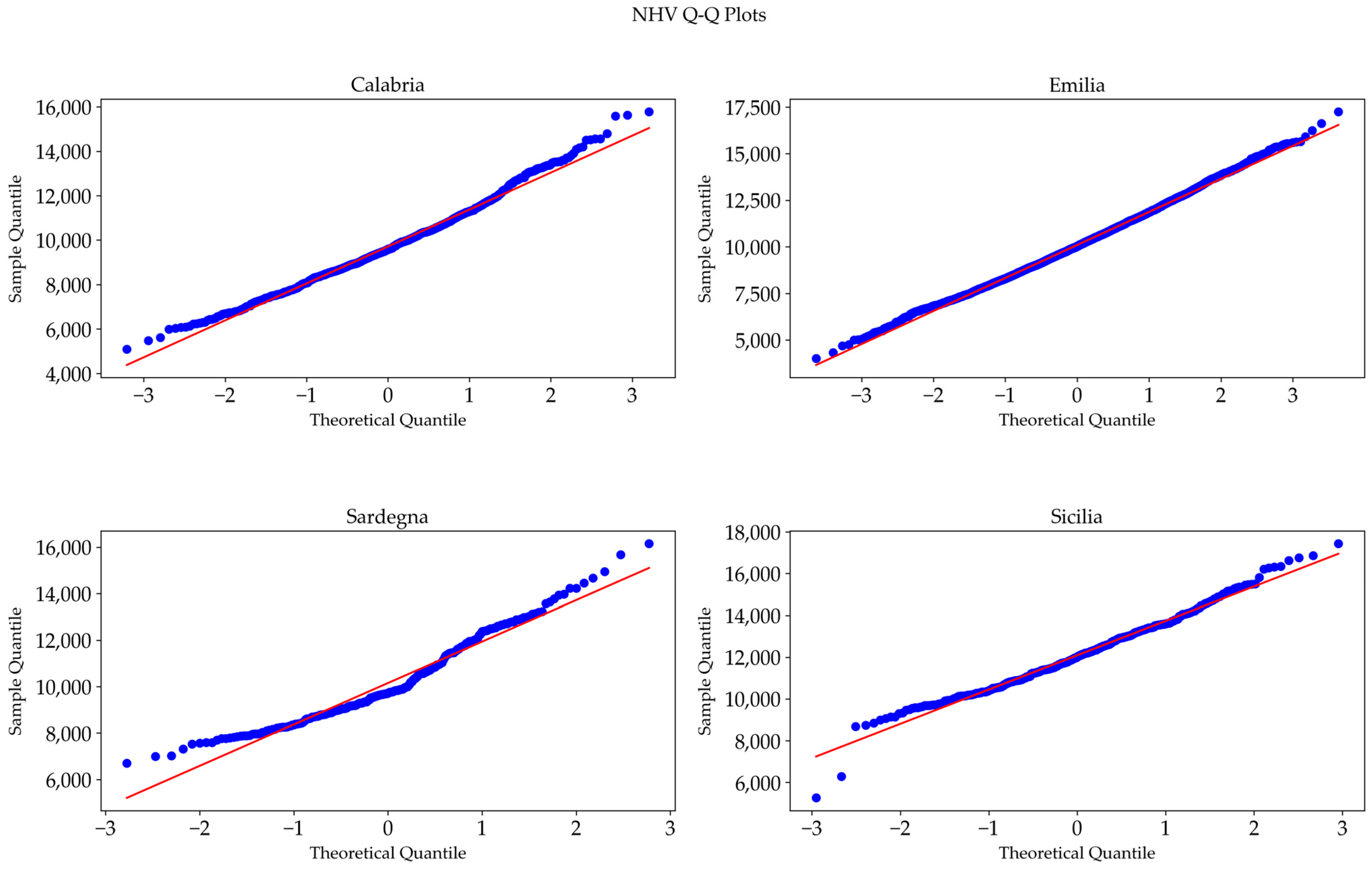
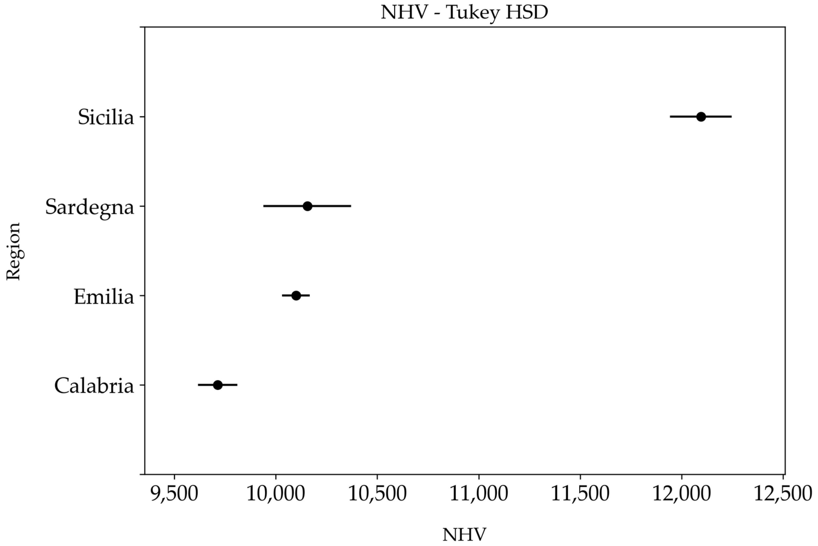
3.1.2. Net Heating Value

A total of 6664 HV analyses were conducted. There were, specifically, 4941 from Emilia-Romagna, 1033 samples from Calabria, 250 from Sardegna, and 440 from Sicilia (

Table 2. Summary of NHV data acquired during the 5-year period. Yearly mean values, as well as yearly quartiles (Q1, Q2, and Q3), are reported as a percentage of as-received mass.

	Net Heating Value (J/g a.r.)
	Year	N. Samples	Mean	St. Dev.	Q1	Q2	Q3
EMILIA - ROMAGNA	2019	315	10,421	1590	9330	10,360	11,556
	2020	800	10,052	1611	9058	10,038	11,020
	2021	1197	10,277	1707	8669	9816	10,966
	2022	1266	10,258	2009	8748	10,207	11,612
	2023	1427	10,086	1733	8885	10,031	11,253
CALABRIA	2019	10	9280	515	8847	9505	9609
		/
	2021	11	11,102	2279	9816	11,588	11,773
	2022	516	9676	1622	8627	9569	10,598
	2023	496	9731	1705	8542	9573	10,840
SARDEGNA	2019	52	10,673	1411	9534	10,423	11,763
	2020	48	11,005	1915	9521	10,707	12,393
	2021	46	10,045	1640	9067	9838	11,013
	2022	58	9669	1946	8311	8832	10,896
	2023	46	9406	1619	8244	8930	9740
SICILIA	2019	94	12,028	1537	10,884	11,712	12,990
	2020	89	11,979	1349	11,018	11,981	12,893
	2021	98	11,746	1767	10,279	11,518	13,381
	2022	91	12,024	1737	10,900	12,108	13,148
	2023	68	12,934	1628	11,710	12,941	13,992

).

As with the MC analysis, the number of samples for NHV analysis received from Emilia-Romagna increased steadily, with the largest increase occurring between 2019 and 2020 when the number of samples increased from 315 up to 800. Between 2019 and 2023, the number of samples increased by 305%. NHV, like MC, due to its correlation, showed annual average variations. The highest annual mean was recorded in 2019 (10,420 J/g, σ = 1590). Despite the reduction of MC values in the following years, NHV did not reach similar values. This may be due to factors in addition to MC, such as the inherent variability in the samples, their number, and the influence of other properties, such as ash content. Between 2020 and 2021, NHV increased by 2.24% from 10,052 J/g (σ = 1610) to 10,277 (σ = 1707) due to the decrease in MC values. In 2022, the average NHV remained unchanged, but in 2023, the NHV decreased slightly by 1.68%. Overall, the NHV decreased by 3.21% between 2019 and 2023, from 10,420 J/g (σ = 1590) to 10,085 J/g (σ = 1733). Finally, the IQR increased by 6.45% over the whole period, indicating increased variability in the data.

For Calabria, the total number of samples analyzed for NHV in the first three years was only 21. This suggests that during the first triennium, NHV was not the main interest of suppliers. However, 516 samples were analyzed in 2022 and 496 in 2023. Between 2022 and 2023, NHV increased slightly by 0.57%, from 9675 J/g (σ = 1621) to 9731 (σ = 1705).

As in the case of MC, Sardegna was the region with the lowest number of samples analyzed for NHV, and the number of samples remained constant over the whole period. As expected, the first two years with the lowest MC values led to the highest NHV, 10,673 J/g (σ = 1411) in 2019 and 11,004 J/g (σ = 1914) in 2020. In the following years, the increase in MC led to a decrease in NHV. In particular, an overall decrease of 12% was observed over the whole 5-year period, reaching 9406 J/g (σ = 1618) in 2023. At the same time, the IQR decreased by 33%, indicating a greater homogeneity of NHVs over time.

The same number of samples from Sicilia analyzed for MC were also analyzed for NHV. As the region whose samples had the lowest MC, the samples analyzed resulted in the highest NHVs. Specifically, NHV increased by 8% over the 5-year period, starting from 12,028 J/g (σ = 1536) and reaching 12,933 J/g (σ = 1627) in 2023. However, the IQR showed strong fluctuations; e.g., in the period 2020–2021, the IQR increased by 65.5%, only to decrease by 27.5% the following year. Overall, the IQR increased by 8% from 2019 to 2023.

The AD test did not reject the null hypothesis of normality, indicating that the NHV data followed a normal distribution, with p-values of 0.78 for Calabria, Emilia-Romagna, and Sicilia and 0.77 for Sardegna. The Q–Q plots confirmed the normality of [39] the data [40,45], although, as expected, given MC’s left-skew [46], they also highlighted a right-skewed tendency for Sardegna (skew = 0.68) and a lighter right-skew tendency in Sicilia’s data (skew = 0.17), indicating a higher frequency of a lower NHV (Figure 3) [41].

A statistically significant difference was observed in the mean NHVs among regions (F = 202.92, p < 0.00). Tukey’s test rejected the null hypothesis for each pair of regions, confirming significant differences except for the Emilia–Sardegna pair (p = 0.96), Ref. [42] with an average NHV of 10,218 J/g (σ = 1730) for the former and 10,159 J/g (σ = 1706) the latter (Figure 4).

The NHV results reflect what was expected from the MC results. In fact, MC has a significant negative effect on the NHV, interfering with the combustion kinetics and reducing the calorific value of the sample [46]. Furthermore, by comparing the Q–Q plots of MC and NHV, it is possible to observe inverse trends in the data distributions, which are concave for MC and convex for NHV, highlighting the inverse correlation between these parameters.

3.1.3. Ash Content

The following ash analyses were carried out on samples from each region during the five-year period: 5356 for Emilia-Romagna, 1259 for Calabria, 250 for Sardegna, and 440 for Sicilia (

Table 3. Summary of ASH data acquired during the 5-year period. Yearly mean values, as well as yearly quartiles (Q1, Q2, and Q3), are reported as percentage of inital dried mass (dried basis, db).

	Ash (% d.b.)
	Year	N. Samples	Mean	St. Dev.	Q1	Q2	Q3
EMILIA - ROMAGNA	2019	504	4.4	2.5	2.8	3.9	5.38
	2020	856	4.4	3.3	2.2	3.8	5.57
	2021	1197	4.7	3.4	2.7	4.2	6.07
	2022	1325	5.1	4.0	2.8	4.1	6.15
	2023	1474	4.9	3.8	2.6	3.9	5.87
CALABRIA	2019	40	4.5	4.2	1.6	2.7	6.6
	2020	36	4.5	7.6	1.8	2.3	3.3
	2021	63	4.8	6.0	2.1	2.9	5.0
	2022	562	4.4	4.1	2.1	3.2	5.2
	2023	558	4.0	3.7	1.9	3.0	4.7
SARDEGNA	2019	52	2.7	1.0	2.0	2.5	3.3
	2020	48	2.7	1.3	1.8	2.8	3.3
	2021	46	3.3	1.9	2.2	3.2	3.9
	2022	58	4.0	2.1	2.6	3.7	4.9
	2023	46	2.9	1.3	1.9	2.8	3.7
SICILIA	2019	94	5.5	2.7	3.6	5.0	6.8
	2020	89	4.9	3.2	3.3	4.1	5.2
	2021	98	6.2	4.2	3.6	4.9	7.1
	2022	91	6.9	3.8	4.5	6.1	7.6
	2023	68	4.8	2.1	3.2	4.5	5.6

).

Throughout the period from 2019 to 2023, the number of samples analyzed for ash in Emilia-Romagna showed a positive trend, increasing from 504 samples in 2019 to 1474 samples in 2023, a significant rise of 192%. The average ASH increased by 11.3% over these years, except for a slight decrease of about 4.0% from 2022 to 2023, where it dropped from an average of 5.1% (σ = 4) to 4.9% (σ = 3.8). Throughout the study period, the median ASH exhibited minimal variation, both positively and negatively, and remained at 3.9% in 2023, the same as in 2019. However, the third quartile values indicated a change from 5.4% in 2019 to 5.9% in 2023, suggesting increased variability in the upper halves of the sample distributions. The annual averages for Emilia-Romagna belong to Class I2, except for 2022, where the increase in the average ash content causes a shift to Class I3.

Regarding the samples from Calabria, from 2019 to 2021, very small quantities were obtained, i.e., between 40 and 60 per year. However, since 2022, there has been an increase in interest in ASH, with 562 samples obtained in 2022 and 558 in 2024. Although the analysis was carried out on a few samples, an increase in its content during the first 3 years has emerged, from 4.5 (σ = 4.2) in 2019 to 4.8 (σ = 6.0) in 2021. In the following years, however, average values decreased sharply, reaching 4.0% (σ = 3.7) in 2023. In contrast, the median value increased in the first three years, rising from 2.7% in 2019 to 2.9% in 2021 and then reaching 3.2% in 2023. Over the whole period, Calabria samples fell into Class I2.

The same samples from Sardegna, tested for NHV throughout the period, were analyzed for ASH. These samples gave the lowest results compared to other regions. In fact, during the first two years, the average ASH was 2.7% (σ = 1.0–1.3), increasing in the following two years to 3.3% (σ = 1.9) and 4% (σ = 2.1). Finally, in 2023, there was a sudden drop to an average of 2.9% (σ = 1.3). The median values followed the same trend, starting at 2.5% and ending at 2.8%. Moreover, the samples from Sardegna shifted from Class I1 for the first two years to Class I2 in 2021 and 2022 and back to Class I1 in 2023.

For Sicilia, the number of samples analyzed for ASH is also the same as for the other parameters. For all years, samples from this region gave higher average values. An example is the year 2019 with a mean ASH of 5.5% (σ = 2.7) or the year 2022 with a mean of 6.9% (σ = 3.8). The same applies to the median values, which are significantly higher than in other regions. Contrary to the MC, the annual average ASH values for Sicilia have always been above I1 threshold values, falling in Class I4 in 2021 and 2022, and back to Class I3 in 2023.

Preliminary statistical analysis combined with the evaluation of the Q–Q plots suggested a deviation of data from normality (Figure 5) [40,45].

Moreover, the data distribution was marked by evident asymmetry with a strong skew to the right. KW highlighted a statistically significant difference between regional median ASH values (H = 263.55, p < 0.00) [47], suggesting substantial variations in ASH among regions beyond what might be expected by chance alone. DT confirmed the difference between each pair of regions (p < 0.00 for each pair), emphasizing the distinctiveness of ash content levels across the regions [48]. As expected, Sicilia was the region with the highest 5-year average results. In fact, the proximity to the sea is one of the main causes of the increase in sodium (Na) and Cl in the biomass, inorganic elements that often form ash, either through aerosols or saltwater intrusion [49]. However, contrary to what might be expected, the samples from Sardegna did not yield the same findings. Thus, other factors may have contributed, such as different agroforestry practices, i.e., removal of bark after felling [50], and the use of different woody species for energy production [51,52].

3.1.4. Nitrogen Content

The total number of analyses of N during the five-year period was 3283, specifically, 2555 from Emilia, 38 from Calabria, 250 from Sardegna, and 440 from Sicilia.

The number of analyses required by suppliers in the Emilia-Romagna region has varied drastically over time. In fact, between 2019 and 2021, the number of analyses increased by approximately 82%, from 450 to 820. This trend is in line with the general increase in demand for analyses in this region. However, in the following years, although the number of analyses for other parameters continues to increase, the focus on N decreases to 281 in 2022 and 335 in 2023. During the first four years, the average nitrogen content varied little, with a minimum of 0.34% (σ = 0.23) in 2022 and a maximum of 0.41% (σ = 0.22) in 2019. In 2023, the average value falls sharply to 0.19% (σ = 0.19). The year 2020 seems to be the year with the highest variation of N values, with an IQR of 0.33, higher than the other years. Due to the low annual averages, the region meets the requirements for Class I1 for N throughout the period.

The number of samples from Calabria turned out to be too few to provide any relevant information. In fact, the year with the most samples analyzed was 2022, with 24 analyses resulting in an average N value of 0.31% (σ = 0.14). Despite the small number of samples analyzed, Calabria’s N complies with Class I1 limits in 2019 and 2022 and with Class I2 in 2021.

From Sardegna, the samples analyzed for ASH and NHV were also analyzed for N. In this case, the average values varied greatly during the first four years, ranging from 0.14% (σ = 0.21) to 0.36% (σ = 0.32). Finally, between 2022 and 2023, there was a clear reduction of 44% to an average value of 0.12% (σ = 0.19) and a median value of 0.18%. Given the consistently low annual averages, the region qualifies for Class I1 for N throughout the entire period.

Again, Sicilia’s samples analyzed for ASH and NHV were also analyzed for N. During the first four years, N values were constant, with a 4-year average of 0.39% (σ = 0.19). However, in 2023, there was a significant decrease in N, dropping to 0.21% (σ = 0.21). A similar trend is observed in the medians, with a 4-year average median of 0.36% and a median of 0.19% for 2023. Lastly, as well as Emilia-Romagna and Sardegna, Sicilia’s N levels comply with Class I1 requirements.

Despite the similar median and mean values indicating a distribution close to normality in almost every case for each region, the Q–Q plot analysis revealed a tendency for the data to deviate from normality (Figure 6). Therefore, non-parametric analysis was preferred over ANOVA.

Thus, KW indicated a statistically significant difference among regional N data (H = 103.62, p < 0.00) [47]. DT pairwise comparisons highlighted that N levels for Sardegna’s samples were distinctively different from those from Calabria, Sicilia, and Emilia-Romagna. Specifically, Sardegna’s N data significantly deviated from Sicilia and Emilia-Romagna with extremely low p-values (p < 0.00), indicating very strong evidence against the null hypothesis. Similarly, the difference between Sardegna and Calabria was statistically significant with a p = 0.02. In contrast, N data between Calabria and Sicilia and Calabria and Emilia-Romagna were not found to be significantly different [48]. Whether or not there was a significant difference between the average N values could have been influenced by many factors. For example, the different composition of the sample, that is, the ratio of the woody fraction to leaf residues, can strongly influence the N value [53] and, as with ASH, the concentration of N can depend on plant species or the soil in which the plant grew.

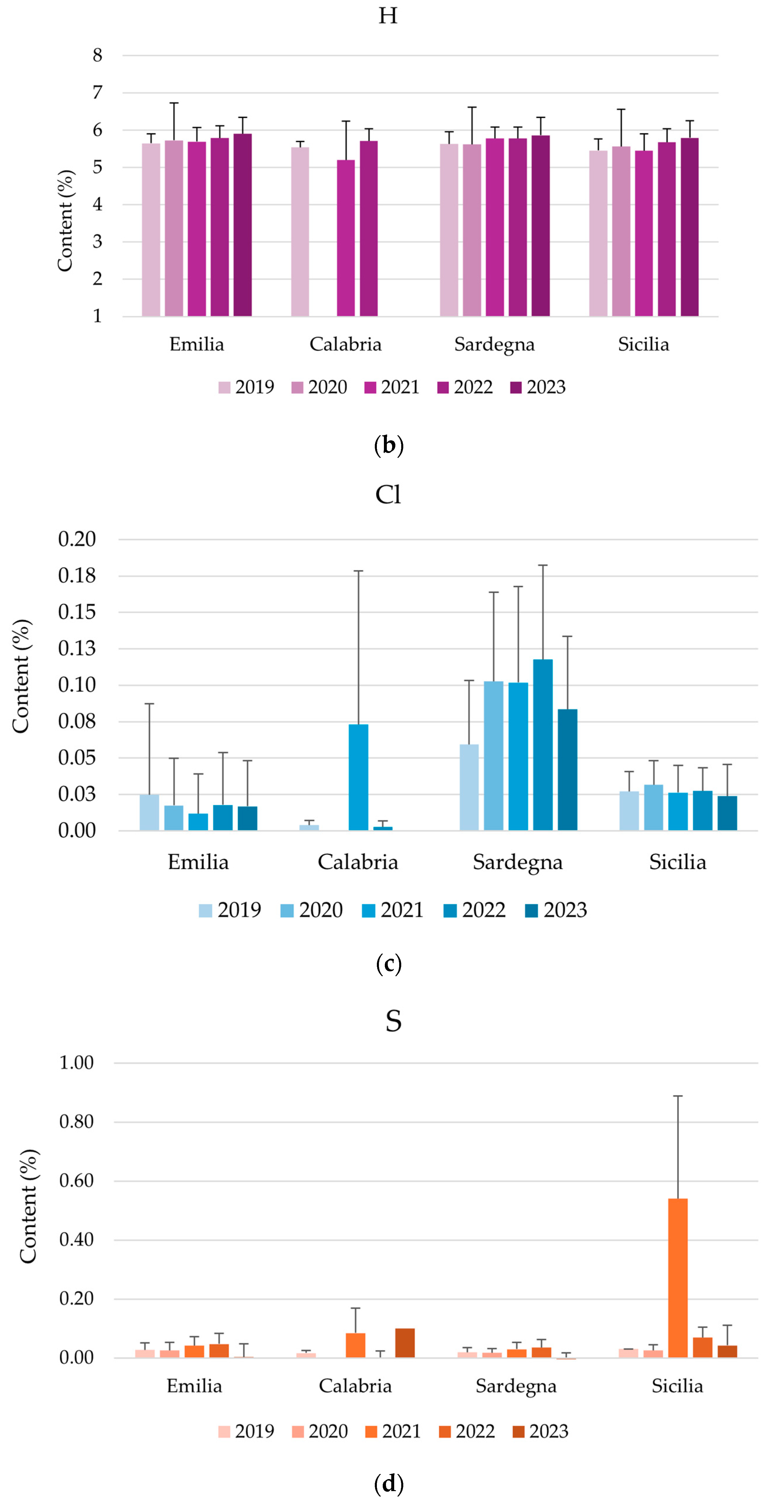
3.1.5. Carbon, Hydrogen, Chlorine, and Sulphur Contents

For each region, particularly in the case of Emilia-Romagna being the region with more analyzed samples, there was no significant change in the C of the samples over time (Figure 7a). The only exception was Calabria with an average C value of 43.9% (σ = 8.6). However, this value does not allow any further conclusions to be drawn due to the small number of samples received, apart from the possible influence of the different types of wood and the different parts of plants used [54]. The same applies to the H value (Figure 7b).

The average Cl values in Emilia-Romagna’s sample were between 0.01% and 0.02% (Figure 7c), while the S values were between 0.0% and 0.04% (Figure 7d). Both parameters therefore remained within Class I1 limits throughout the five-year period. The other regions, on the contrary, showed mixed results. For example, in 2021, samples from Calabria presented Cl values falling into Class I3 (0.07%, σ = 0.1) and I2 for S values (0.08%, σ = 0.08). However, even in this case, the small number of samples does not allow an in-depth analysis of the results.

Also, for Sardegna’s samples, Cl fell in Class I3 in 2020 and 2021 (0.10%, σ = 0.06), while in 2022, it fell in Class I4 (0.11%, σ = 0.06). S values, on the other hand, always remained low, ranging from 0.01% and 0.03%. Sicilia’s samples, on the other hand, presented fluctuating Cl values, between 0.02% and 0.03%, while S fluctuated between 0.02% in the first two years and increased to 0.54%, excluding itself from any Class in 2021. The particularly high Cl values for the samples from Sardegna and Sicilia may be due to the proximity of the supply area to the sea. However, the variability in the data in the same regions also seems to indicate a variation in the inter-regional geographical areas from which the biomass originates [55]. The same reason, as well as the different management of the areas from which the biomasses were harvested, could explain the variability in the average S value as well [56].

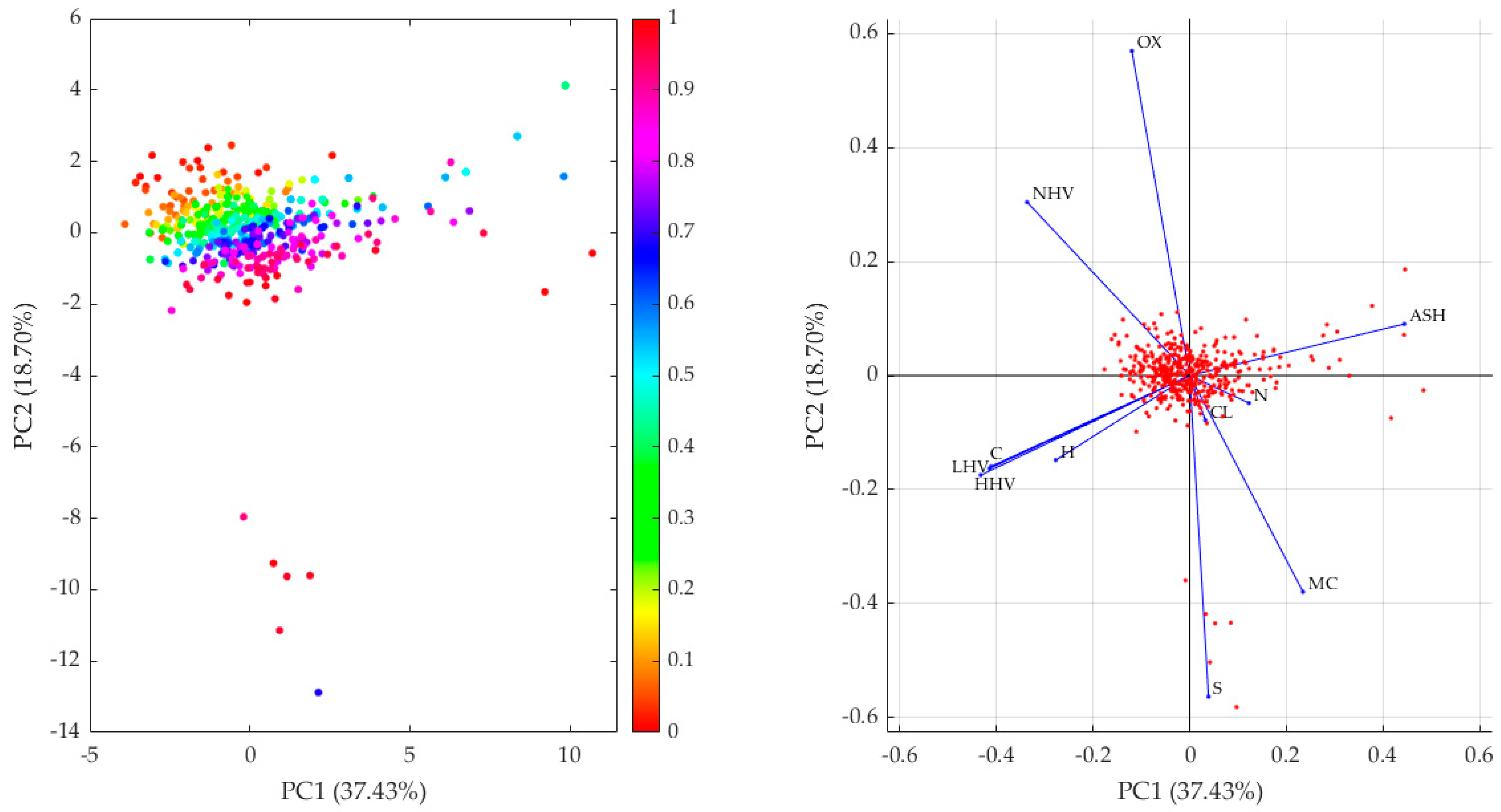
3.2. Multivariate Analysis Results

The large amount of data resulted in an in-depth evaluation of each considered region (

Table 4. Number of samples with comprehensive results considered for each investigation according to the (A) Spatial Analysis (SA) and (B) Temporal Analysis (TA).

Macro Division	Database	N. Samples
SA	2019	338
	2020	490
	2021	687
	2022	363
	2023	409
TA	Emilia	1699
	Calabria	38
	Sardegna	110
	Sicilia	440

), with the exception of Calabria due to the smaller number of samples available with complete data as a result of the more restricted analyses required by the suppliers. As a result, Calabria’s matrix was unable to provide a sufficient amount of data for reliable exploration, resulting in a weaker performance compared to other regions.

For both the SA and TA, a clear separation between samples was observed regarding MC variation, which is considered to be one of the most discriminating parameters for qualitative characterization. Furthermore, the study of the corresponding loading plot showed a strong negative correlation between MC and NHV, proving the negative influence of water on energy yield [57]. Moreover, a negative correlation between ASH and higher heating value (HHV), confirms its role in reducing combustion efficiency [58]. The lower heating value (LHV) always followed the HHV, thereby providing a strong correlation.

Little differences were detected in specific investigations of the other parameters. In the case of the SA, in 2019 and 2020, C and H showed a direct and relevant correlation with the calorific values, while an inverse relation was observed for N and S. Moreover, ASH was inversely correlated with O, while Cl showed an important negative correlation with MC despite the stronger influence of the NHV. In 2020′s data, ASH and N were strongly correlated, while S lost its correlation with N. In 2021 (Figure 8), O showed a negative correlation with ASH, as well as H and S, which maintained a negative correlation. No relevant correlations were detected between Cl, N, and S. Lastly, for 2022, Cl, S, N, and H parameters showed less influence in sample separation, while O, C, and heating values maintained a negative correlation with ASH.

For the TA, Calabria and Sardegna’s data was not considered due to the lack of sufficient information. In the case of Emilia-Romagna’s data (Figure 9), an inverse correlation was found between ASH and heating values, C and O, while N, S, and Cl showed no relevance in the distribution.

In Sicilia’s case (Figure 10), O and S revealed an important inverse correlation, as well as NHV and MC. Moreover, few observations showed a value of S as the greatest discriminant variable. Cl and N parameters were not relevant for sample distribution, while H followed HHV and LHV, thus showing an inverse correlation with ASH. Also, in this case, a small group of samples have distinguished compared to the other observations with higher values in some variables.

Nevertheless, in each PCA investigation, the PCs explained approximately 50% of the total variance in the data set. In fact, the inherent variability in industrial woodchips, coupled with the demanding requirements of the sampling procedure, could have influenced and enhanced the variance between observations, resulting in rare and extreme results that enhance a scatter distribution.

Along with the biplot, Pearson’s analyses also allowed to confirm the degree of linear correlation between the variables, thus supporting the identification of more discriminating variables. Pearson’s analysis was carried out only on the TA data, assuming an internal variation of the correlations between years for a given region. That is, the SA database, based on the fusion of each year with data from all the regions, would not have made it possible to identify which region had the greatest influence on the others, thus limiting a complete description. Therefore, in accordance with the results of the PCA, Emilia-Romagna (

Table 5. Pearson’s analysis on the Emilia dataset. The different scale of green indicates the main interesting degree of correlation in descendant order from dark green (higher correlation) to light green (lower correlation). The grey boxes explain the perfect linear correlation between the same parameter along the principal diagonal.

Variable	MC	NHV	ASH	HHV	LHV	C	H	N	OX	CL	S
MC	1.000
NHV	−0.961	1.000
ASH	0.021	−0.223	1.000
HHV	0.091	0.164	−0.802	1.000
LHV	0.094	0.181	−0.743	0.941	1.000
C	0.014	0.144	−0.628	0.624	0.580	1.000
H	−0.012	−0.057	−0.142	0.137	−0.205	0.109	1.000
N	−0.021	−0.056	0.332	−0.304	−0.272	−0.274	−0.083	1.000
OX	−0.031	0.148	−0.536	0.309	0.410	−0.247	−0.315	−0.183	1.000
CL	−0.125	0.108	0.099	−0.064	−0.052	−0.035	−0.033	0.106	−0.086	1.000
S	−0.069	0.033	0.208	−0.139	−0.132	−0.076	−0.016	0.177	−0.193	0.173	1.000

) and Sicilia’s (

Table 6. Pearson’s analysis on the Sicilia dataset. The different scale of green indicates the main interesting degree of correlation in descendant order from dark green (higher correlation) to light green (lower correlation). The grey boxes explain the perfect linear correlation between the same parameter along the principal diagonal.

	MC	NHV	ASH	HHV	LHV	C	H	N	OX	CL	S
MC	1.000
NHV	−0.956	1.000
ASH	0.285	−0.478	1.000
HHV	−0.127	0.407	−0.789	1.000
LHV	−0.115	0.399	−0.754	0.992	1.000
C	−0.226	0.397	−0.764	0.697	0.650	1.000
H	−0.126	0.192	−0.516	0.390	0.273	0.583	1.000
N	0.138	−0.148	0.176	−0.107	−0.089	−0.184	−0.171	1.000
OX	−0.250	0.266	−0.214	0.112	0.120	−0.012	−0.022	−0.062	1.000
CL	−0.011	0.013	0.075	−0.012	−0.007	−0.033	−0.040	0.224	−0.099	1.000
S	0.149	−0.127	−0.046	0.044	0.044	−0.007	0.017	0.007	−0.831	0.081	1.000

) data were investigated.

In both cases, a significant negative correlation between MC and NHV and a positive correlation between HHV and LHV have been observed. Furthermore, ASH correlated with C (slightly lower in Emilia-Romagna’s case than in Sicilia, r = −0.63 and r = −0.76, respectively) and with O in Emilia-Romagna’s case (r = −0.54). While ASH showed a negative correlation with H in the case of Sicilia (r = −0.52), a significant negative correlation between O and S (r = −0.83) was found only in the Sicilia dataset, which probably corresponded to the sample group separated by high S.

3.3. Closing Discussion

In the form of thematic maps (Figure 11), an overall summary of the results is proposed, in particular, for the main quality parameters.

This study shows a significant increase in the number of samples analyzed from Emilia-Romagna, indicating a growing interest or capacity in sample collection or analysis over time. Despite variations, MC remained within acceptable limits for quality Class I1 throughout the study period. NHVs showed variations in the annual averages, with the highest average recorded in 2019 at 10,420 J/g. Interestingly, while MC decreased during the years, the NHV did not follow compatible trends, suggesting that factors beyond MC, such as inherent sample variability and other properties, may influence NHV measurements. From 2019 to 2023, Emilia-Romagna experienced a significant increase in the number of samples analyzed for ASH. The region generally maintained quality Class I2 each year, except in 2022, when higher average ash content temporarily shifted it to Class I3, indicating the need for continued vigilance in maintaining product quality standards. While there has been variability in the demand for N analysis over the years, Emilia-Romagna has demonstrated overall adherence to quality standards, ensuring products meet regulatory requirements despite these fluctuations.

The analysis of samples from Calabria shows significant variability in the number of samples analyzed, with a notable decrease in 2020 followed by a sharp increase in 2022, culminating in a 382% increase from 2019 to 2023. MC, consistently higher than in Emilia-Romagna, peaked at 46.5% in 2020 but decreased to 41% in 2023. Despite the variability, the MC values always met the I1 quality standards, except for the first two years when they were classified as I2. This trend highlights Calabria’s efforts to maintain quality standards in the face of changing sample volumes and moisture conditions. In Calabria, the number of samples analyzed for NHV was minimal in the first three years, totaling only 21 samples. This suggests that NHV was not initially a major focus for suppliers. However, there was a significant increase with 516 samples analyzed in 2022 and 496 in 2023. There was also a significant increase in interest in ASH levels from 2022 onwards, in contrast to the minimal number of samples analyzed in previous years. Despite fluctuations, ASH values were generally within the I2 quality standards throughout the period. The analysis of N was carried out on limited samples until 2022, with only 24 samples analyzed in that year. Nevertheless, N consistently met the quality standards and was classified as Class I1 in 2019 and 2022 and as Class I2 in 2021.

Both Sardegna and Sicilia demonstrated trends of stable or decreasing sample sizes over the years, with distinct patterns in moisture content levels. While Sardegna showed increasing MC levels with reduced variability, Sicilia maintained consistently lower MC levels with improved uniformity among samples. Both regions maintained adherence to quality standards throughout the period, highlighting their commitment to maintaining product integrity in agricultural samples. While Sardegna experienced consistent NHVs with a downward trend over time due to increasing MC levels, Sicilia consistently produced samples with the highest NHVs. However, the variability in NHVs, as indicated by fluctuations in the IQR, suggests potential influences from other factors such as sample diversity or analytical methods. While Sardegna’s ASH displayed variability and compliance with quality standards over time, Sicilia consistently exhibited higher ASH values that occasionally exceeded standard thresholds. These insights underscore the importance of ongoing analysis and monitoring to understand and maintain quality standards in agricultural products across different regions. Both Sardegna and Sicilia demonstrate variability in nitrogen content over the years; however, despite these fluctuations, both regions maintained compliance with Class I1 standards for nitrogen content throughout the study period, indicating consistent adherence to quality standards in agricultural products.

As for the other parameters, Emilia-Romagna consistently maintained C and H values without significant changes over the study period. Cl and S values remained within Class I1 limits throughout the five years. In contrast, Calabria and Sardegna showed variable Cl and S values, occasionally exceeding Class I1 standards due to regional factors like proximity to the sea and varied biomass sourcing areas. Sicilia exhibited fluctuating Cl values and an increase in S values, impacting its classification over the years.

4. Conclusions

An increased focus on quality monitoring in Italy was observed, reflected in an increase in the number of samples received from suppliers and an overall improvement in the average quality parameter. Results suggest that companies are increasingly focusing on quality control, closely linked to quality improvement, consequently having a positive influence on sustainability.

The five-year data revealed an overall reduction in MC and N, while ASH and NHV showed non-linear fluctuations. The decline in MC may be linked to climate change, however, to verify this hypothesis further studies are needed. Different practices may explain statistically significant differences in quality between samples from different regions [59,60]. For example, outdoor versus indoor storage can affect MC, just as storage in marshy areas can affect Cl and S content [61,62]. Cl and S could also be affected by differing conditions under which biomass grows, such as proximity to the sea [63,64]. In addition, the way in which biomass is extracted from forests, such as by dragging logs, can also result in the presence of inert components that inevitably increase ASH.

While this work provided an overview of the quality of woody biomass over time and over four macro-areas in Italy, more data could be sought on the exact source, i.e., the harvesting areas, of the biomass. This would allow for a comprehensive mapping of the different lignocellulosic biomasses across the country. However, this might prove difficult, as it would involve large-scale work to which the many different biomass suppliers would have to consent, providing accurate and continuous data, and enabling extensive tracking of biomasses’ quality. This obstacle could be overcome by an evolution of national incentives concerning the promotion of biomass quality and sustainability.

References

1. Report from the Commission to the European Parliament, the Council, the European Economic and Social Committee and the Committee of the Regions—State of the Energy Union Report 2023 (Pursuant to Regulation (EU) 2018/1999 on the Governance of the Energy Union and Climate Action), Brussel. Available online: https://eur-lex.europa.eu/legal-content/EN/TXT/?uri=CELEX%3A52023DC0650 (accessed on 14 June 2024).
2. Toscano, G.; De Francesco, C.; Gasperini, T.; Fabrizi, S.; Duca, D.; Ilari, A. Quality Assessment and Classification of Feedstock for Bioenergy Applications Considering ISO 17225 Standard on Solid Biofuels. Resources 2023, 12, 69. [Google Scholar] [CrossRef]
3. Eurostat Data Browser—Volume of Timber (FAO, FE). Available online: https://ec.europa.eu (accessed on 15 June 2024).
4. Eurostat Data Browser—Area of Wooded Land (FAO, FE). Available online: https://ec.europa.eu (accessed on 14 June 2024).
5. Moliner, C.; Marchelli, F.; Arato, E. Current Status of Energy Production from Solid Biomass in North-West Italy. Energies 2020, 13, 4390. [Google Scholar] [CrossRef]
6. Moliner, C.; Arato, E.; Marchelli, F. Current Status of Energy Production from Solid Biomass in Southern Italy. Energies 2021, 14, 2576. [Google Scholar] [CrossRef]
7. Del Giudice, A.; Scarfone, A.; Paris, E.; Gallucci, F.; Santangelo, E. Harvesting Wood Residues for Energy Production from an Oak Coppice in Central Italy. Energies 2022, 15, 9444. [Google Scholar] [CrossRef]
8. Proto, A.R.; Macrì, G.; Visser, R.; Harrill, H.; Russo, D.; Zimbalatti, G. Factors Affecting Forwarder Productivity. Eur. J. Res. 2018, 137, 143–151. [Google Scholar] [CrossRef]
9. European Commission. Directorate-General for Research and Innovation, European Green Deal—Research & Innovation Call; Publications Office of the European Union: Luxembourg, 2021.
10. Diego, R.; Giorgio, M.; Giuseppe, L.; Alessandro, D.R. Wood Energy Plants and Biomass Supply Chain in Southern Italy. Procedia Soc. Behav. Sci. 2016, 223, 849–856. [Google Scholar] [CrossRef]
11. La Scalia, G.; Adelfio, L.; La Fata, C.M.; Micale, R. Economic and Environmental Assessment of Biomass Power Plants in Southern Italy. Sustainability 2022, 14, 9676. [Google Scholar] [CrossRef]
12. He, J.; Liu, Y.; Lin, B. Should China Support the Development of Biomass Power Generation? Energy 2018, 163, 416–425. [Google Scholar] [CrossRef]
13. Evans, A.; Strezov, V.; Evans, T.J. Sustainability Considerations for Electricity Generation from Biomass. Renew. Sustain. Energy Rev. 2010, 14, 1419–1427. [Google Scholar] [CrossRef]
14. Jåstad, E.O.; Bolkesjø, T.F.; Trømborg, E.; Rørstad, P.K. The Role of Woody Biomass for Reduction of Fossil GHG Emissions in the Future North European Energy Sector. Appl. Energy 2020, 274, 115360. [Google Scholar] [CrossRef]
15. Sulaiman, C.; Abdul-Rahim, A.S.; Ofozor, C.A. Does Wood Biomass Energy Use Reduce CO2 Emissions in European Union Member Countries? Evidence from 27 Members. J. Clean. Prod. 2020, 253, 119996. [Google Scholar] [CrossRef]
16. Antar, M.; Lyu, D.; Nazari, M.; Shah, A.; Zhou, X.; Smith, D.L. Biomass for a Sustainable Bioeconomy: An Overview of World Biomass Production and Utilization. Renew. Sustain. Energy Rev. 2021, 139, 110691. [Google Scholar] [CrossRef]
17. Reijnders, L. Conditions for the Sustainability of Biomass Based Fuel Use. Energy Policy 2006, 34, 863–876. [Google Scholar] [CrossRef]
18. Klavina, A.; Selegovskis, R. Influence of Wood Chip Quality on Boiler House Efficiency. Eng. Rural. Dev. 2021, 20, 393–398. [Google Scholar] [CrossRef]
19. Schön, C.; Kuptz, D.; Mack, R.; Zelinski, V.; Loewen, A.; Hartmann, H. Influence of Wood Chip Quality on Emission Behaviour in Small-Scale Wood Chip Boilers. Biomass Convers. Biorefin. 2019, 9, 71–82. [Google Scholar] [CrossRef]
20. Proto, A.R.; Palma, A.; Paris, E.; Papandrea, S.F.; Vincenti, B.; Carnevale, M.; Guerriero, E.; Bonofiglio, R.; Gallucci, F. Assessment of Wood Chip Combustion and Emission Behavior of Different Agricultural Biomasses. Fuel 2021, 289, 119758. [Google Scholar] [CrossRef]
21. Dzurenda, L.; Banski, A. The Effect of Firewood Moisture Content on the Atmospheric Thermal Load by Flue Gases Emitted by a Boiler. Sustainability 2019, 11, 284. [Google Scholar] [CrossRef]
22. Chen, Q.; Zhang, X.; Zhou, J.; Sharifi, V.N.; Swithenbank, J. Effects of Flue Gas Recirculation on Emissions from a Small Scale Wood Chip Fired Boiler. Phys. Procedia 2015, 66, 65–68. [Google Scholar] [CrossRef]
23. DBFZ (Deutsches Biomasseforschungszentrum Gemeinnützige GmbH). Model Contract for Biomass Delivery. Horizon 2020 Coordination and Support Action No. 646495: Bioenergy for Business. Uptake of Solid Bioenergy in European Commercial Sectors. 2015. Available online: https://ec.europa.eu/research/participants/documents/downloadPublic?documentIds=080166e5a191c345&appId=PPGMS (accessed on 14 June 2024).
24. Lieskovský, M.; Jankovský, M.; Trenčiansky, M.; Merganič, J.; Dvořák, J. Ash Content vs. the Economics of Using Wood Chips for Energy: Model Based on Data from Central Europe. Bioresources 2017, 12, 1579–1592. [Google Scholar] [CrossRef]
25. ISO 17225-1:2014; Solid Biofuels: Fuel Specifications and Classes. International Organization for Standardization: Geneva, Switzerland, 2014.
26. ISO 17225-9:2019; Solid Biofuels: Fuel Specifications and Classes—Part 9: Graded Hog Fuel and Wood Chips for Industrial Use. International Organization for Standardization: Geneva, Switzerland, 2014.
27. ISO 18134; Solid Biofuels-Determination of Moisture Content-Oven Dry Method-Part 2. International Organization for Standardization: Geneva, Switzerland, 2015.
28. ISO 18122; Solid Biofuels-Determination of Ash Content. International Organization for Standardization: Geneva, Switzerland, 2015.
29. ISO 18125; Solid Biofuels-Determination of Calorific Value. International Organization for Standardization: Geneva, Switzerland, 2017.
30. ISO 16948; Solid Biofuels-Determination of Total Content of Carbon, Hydrogen and Nitrogen. International Organization for Standardization: Geneva, Switzerland, 2015.
31. ISO 16994; Solid Biofuels-Determination of Total Content of Sulfur and Chlorine. International Organization for Standardization: Geneva, Switzerland, 2015.
32. McKinney, W. Data Structures for Statistical Computing in Python. In Proceedings of the 9th Python in Science Conference 2010, Austin, TX, USA, 28–30 June 2010; pp. 56–61. [Google Scholar] [CrossRef]
33. Virtanen, P.; Gommers, R.; Oliphant, T.E.; Haberland, M.; Reddy, T.; Cournapeau, D.; Burovski, E.; Peterson, P.; Weckesser, W.; Bright, J.; et al. SciPy 1.0: Fundamental Algorithms for Scientific Computing in Python. Nat. Methods 2020, 17, 261–272. [Google Scholar] [CrossRef] [PubMed]
34. Hunter, J.D. Matplotlib: A 2D Graphics Environment. Comput. Sci. Eng. 2007, 9, 90–95. [Google Scholar] [CrossRef]
35. Seabold, S.; Perktold, J. Statsmodels: Econometric and Statistical Modeling with Python. In Proceedings of the 9th Python in Science Conference 2010, Austin, TX, USA, 28–30 June 2010; pp. 92–96. [Google Scholar] [CrossRef]
36. Toscano, G.; Rinnan, Å.; Pizzi, A.; Mancini, M. The Use of Near-Infrared (NIR) Spectroscopy and Principal Component Analysis (PCA) to Discriminate Bark and Wood of the Most Common Species of the Pellet Sector. Energy Fuels 2017, 31, 2814–2821. [Google Scholar] [CrossRef]
37. Popescu, C.M.; Navi, P.; Placencia Peña, M.I.; Popescu, M.C. Structural Changes of Wood during Hydro-Thermal and Thermal Treatments Evaluated through NIR Spectroscopy and Principal Component Analysis. Spectrochim. Acta A Mol. Biomol. Spectrosc. 2018, 191, 405–412. [Google Scholar] [CrossRef] [PubMed]
38. Jorgensen, A. Clustering Excipient Near Infrared Spectra Using Different Chemometric Methods; Technical Report; Department of Pharmacy, University of Helsinki: Helsinki, Finland, 2000. [Google Scholar]
39. Anderson, T.W.; Darling, D.A. A Test of Goodness of Fit. J. Am. Stat. Assoc. 1954, 49, 765–769. [Google Scholar] [CrossRef]
40. Kozak, M.; Piepho, H.P. What’s Normal Anyway? Residual Plots Are More Telling than Significance Tests When Checking ANOVA Assumptions. J. Agron. Crop Sci. 2018, 204, 86–98. [Google Scholar] [CrossRef]
41. Doane, D.P.; Seward, L.E. Measuring Skewness: A Forgotten Statistic? J. Stat. Educ. 2011, 19. [Google Scholar] [CrossRef]
42. Nanda, A.; Mohapatra, B.B.; Mahapatra, A.P.K.; Mahapatra, A.P.K.; Mahapatra, A.P.K. Multiple Comparison Test by Tukey’s Honestly Significant Difference (HSD): Do the Confident Level Control Type I Error. Int. J. Stat. Appl. Math. 2021, 6, 59–65. [Google Scholar] [CrossRef]
43. Salminen, J.; Sairanen, H.; Patel, S.; Ojanen-Saloranta, M.; Kajastie, H.; Palkova, Z.; Heinonen, M. Effects of Sample Handling and Transportation on the Moisture Content of Biomass Samples. Int. J. Thermophys. 2018, 39, 66. [Google Scholar] [CrossRef]
44. ISO 18135:2017; Solid Biofuels-Sampling BSI Standards Publication. International Organization for Standardization: Geneva, Switzerland, 2017.
45. Q-Q Plot (Quantile to Quantile Plot). The Concise Encyclopedia of Statistics; Springer: New York, NY, USA, 2008; pp. 437–439. [Google Scholar] [CrossRef]
46. Demirbas, A. Effects of Moisture and Hydrogen Content on the Heating Value of Fuels. Energy Sources Part A Recovery Util. Environ. Eff. 2007, 29, 649–655. [Google Scholar] [CrossRef]
47. McKight, P.E.; Najab, J. Kruskal-Wallis Test. The Corsini Encyclopedia of Psychology; John Wiley & Sons: Hoboken, NJ, USA, 2010; p. 1. [Google Scholar] [CrossRef]
48. Dunn, O.J. Multiple Comparisons Using Rank Sums. Technometrics 1964, 6, 241–252. [Google Scholar] [CrossRef]
49. Vassilev, S.V.; Vassileva, C.G.; Song, Y.C.; Li, W.Y.; Feng, J. Ash Contents and Ash-Forming Elements of Biomass and Their Significance for Solid Biofuel Combustion. Fuel 2017, 208, 377–409. [Google Scholar] [CrossRef]
50. Nosek, R.; Holubcik, M.; Jandacka, J. The Impact of Bark Content of Wood Biomass on Biofuel Properties. Bioresources 2016, 11, 44–53. [Google Scholar] [CrossRef]
51. Guidi, W.; Piccioni, E.; Ginanni, M.; Bonari, E. Bark Content Estimation in Poplar (Populus deltoides L.) short-rotation coppice in Central Italy. Biomass Bioenergy 2008, 32, 518–524. [Google Scholar] [CrossRef]
52. Röser, D.; Mola-Yudego, B.; Sikanen, L.; Prinz, R.; Gritten, D.; Emer, B.; Väätäinen, K.; Erkkilä, A. Natural Drying Treatments during Seasonal Storage of Wood for Bioenergy in Different European Locations. Biomass Bioenergy 2011, 35, 4238–4247. [Google Scholar] [CrossRef]
53. Maslova, S.P.; Tabalenkova, G.N.; Golovko, T.K. Respiration and Nitrogen and Carbohydrate Contents in Perennial Rhizome-Forming Plants as Related to Realization of Different Adaptive Strategies. Russ. J. Plant Physiol. 2010, 57, 631–640. [Google Scholar] [CrossRef]
54. Bārdule, A.; Liepiņš, J.; Liepiņš, K.; Stola, J.; Butlers, A.; Lazdiņš, A. Variation in Carbon Content among the Major Tree Species in Hemiboreal Forests in Latvia. Forests 2021, 12, 1292. [Google Scholar] [CrossRef]
55. Lee, J.S.; Ghiasi, B.; Lau, A.K.; Sokhansanj, S. Chlorine and Ash Removal from Salt-Laden Woody Biomass by Washing and Pressing. Biomass Bioenergy 2021, 155, 106272. [Google Scholar] [CrossRef]
56. Han, K.; Gao, J.; Qi, J. The Study of Sulphur Retention Characteristics of Biomass Briquettes during Combustion. Energy 2019, 186, 115788. [Google Scholar] [CrossRef]
57. Toscano, G.; Leoni, E.; Gasperini, T.; Picchi, G. Performance of a Portable NIR Spectrometer for the Determination of Moisture Content of Industrial Wood Chips Fuel. Fuel 2022, 320, 123948. [Google Scholar] [CrossRef]
58. Leoni, E.; Mancini, M.; Duca, D.; Toscano, G. Rapid Quality Control of Woodchip Parameters Using a Hand-Held Near Infrared Spectrophotometer. Processes 2020, 8, 1413. [Google Scholar] [CrossRef]
59. Nimitpaitoon, T.; Sajjakulnukit, B.; Prangbang, P. The Effect of Storage Conditions on the Characteristics of Various Types of Biomass. Int. J. Adv. Appl. Sci. 2023, 10, 130–139. [Google Scholar] [CrossRef]
60. Brand, M.A.; Bolzon de Muñiz, G.I.; Quirino, W.F.; Brito, J.O. Storage as a Tool to Improve Wood Fuel Quality. Biomass Bioenergy 2011, 35, 2581–2588. [Google Scholar] [CrossRef]
61. Parzych, A.; Mochnacký, S.; Sobisz, Z.; Polláková, N.; Šimanský, V. Needles and Bark of Picea abies (L.) H. Karst and Picea omorika (Pančiç) Purk. as Bioindicators of Environmental Quality. Folia For. Pol. Ser. A—For. 2018, 60, 230–240. [Google Scholar] [CrossRef]
62. Werkelin, J.; Skrifvars, B.J.; Hupa, M. Ash-Forming Elements in Four Scandinavian Wood Species. Part 1: Summer Harvest. Biomass Bioenergy 2005, 29, 451–466. [Google Scholar] [CrossRef]
63. Svensson, T.; Löfgren, A.; Saetre, P.; Kautsky, U.; Bastviken, D. Chlorine Distribution in Soil and Vegetation in Boreal Habitats along a Moisture Gradient from Upland Forest to Lake Margin Wetlands. Environ. Sci. Technol. 2023, 57, 11067–11074. [Google Scholar] [CrossRef]
64. Patel, B.; Gami, B.; Patel, P. The Leaching of Soluble Chloride from Terrestrial and Water-Based Biomass. Energy Sources Part A Recovery Util. Environ. Eff. 2012, 34, 2280–2286. [Google Scholar] [CrossRef]
Figure 1. Quantile–quantile plots of MC data. The blue points represent individual data values, while the red line represents the theoretical normal distribution. Calabria and Emilia-Romagna (Emilia) dots fit the theoretical normal distribution almost perfectly. Sardegna and Sicilia show a slight deviation from normality (both in the upper and lower part of the distribution of the dots), but almost all the dots remain on the theoretical normal distribution line, confirming the normality of the data set.
Resources 13 00115 g001
Figure 2. Multiple comparison test highlighting the difference among regional annual mean values except for Sardegna and Emilia-Romagna. Black dots indicate the 5-yearly period mean regional values, while lines indicate the confidence intervals for the mean differences, whereas non-overlapping intervals indicate significant differences.
Resources 13 00115 g002
Figure 3. Quantile–quantile plots of NHV data. The blue points represent individual data values, while the red line represents the theoretical normal distribution. Calabria and Emilia-Romagna (Emilia) points fit the theoretical normal distribution almost perfectly. Sardegna and Sicilia show a slight right-skewing of the data, highlighted by the ends of the dataset (blue dots) above the theoretical line.
Resources 13 00115 g003
Figure 4. Multiple comparison test highlighing the difference among regional annual mean values except for Sardegna and Emilia-Romagna. Black dots indicate the 5-yearly period mean regional values, while lines indicate the confidence intervals for the mean differences, whereas non-overlapping intervals indicate significant differences.
Resources 13 00115 g004
Figure 5. Quantile–quantile plots of ASH data. The blue points represent individual data values, while the red line represents the theoretical normal distribution. The data from each region resulted in an upward-sloping curve, indicating a deviation from normality, specifically a right-skew of the data.
Resources 13 00115 g005
Figure 6. Quantile–quantile plots of N data. The blue points represent individual data values, while the red line represents the theoretical normal distribution. As for ASH data, N data from each region resulted in an upward-sloping curve, indicating a deviation from normality, specifically a right-skewing of the data.
Resources 13 00115 g006
Figure 7. Histograms of C (a), H (b), Cl (c), and S (d) contents, showing annual means expressed as percentages on a dry basis and standard deviations. As for C (a) and H (b), there were no significant differences between the regions, except for Calabria, but the data do not allow any further conclusions to be drawn due to the small number of samples received. Sardinia seems to be the region with a higher Cl (c) content, probably due to the geographical area. S (d) content seems to be constant among the regions, with the exception of 2021 in Sicily.
Resources 13 00115 g007aResources 13 00115 g007b
Figure 8. The corresponding score plot (on the left) and biplot (on the right) of the 2021 dataset. The score plot represents the zoomed distribution of the samples reported in the biplot. Moreover, the graduated scale of score plot is based on the MC variation, using the values from 0 to 1 to respectively indicate the lowest and the highest MC result.
Resources 13 00115 g008
Figure 9. The corresponding score plot (on the left) and biplot (on the right) of the Emilia dataset. The score plot represents the zoomed distribution of the samples reported in the biplot. Moreover, the graduated scale of score plot is based on the MC variation, using the values from 0 to 1 to respectively indicate the lowest and the highest MC result.
Resources 13 00115 g009
Figure 10. The corresponding score plot (on the left) and biplot (on the right) of the Sicilia dataset. The score plot represents the zoomed distribution of the samples reported in the biplot. Moreover, the graduated scale of the score plot is based on the MC variation, using the values from 0 to 1 to respectively indicate the lowest and the highest MC result.
Resources 13 00115 g010
Figure 11. Thematic maps summarizing the evolution of MC, NHV, and ASH values over the years.
Resources 13 00115 g011aResources 13 00115 g011bResources 13 00115 g011c