Assessing the Relationship Between Production and Land Transformation for Chilean Copper Mines Using Satellite and Operational Data

Abstract

Mining may cause devastating environmental impacts through large-scale land transformations. However, mining-induced land transformations are poorly understood relative to a mine’s productivity or life cycle. We integrated satellite imagery, geographic information systems (GISs), and mine site production data (ore, concentration, and waste) to conduct a detailed spatiotemporal analysis of 15 open-pit copper mines in Chile, distinguishing six types of features. Although the occupied area (9.90 to 149.61 km² in 2020) and composition vary across mines, facilities for waste storage occupy the largest proportion (>50%) of the transformed land area, emphasizing the need for proper waste management. The analysis of land transformation factors (the transformed land area per unit production) showed high variation (0.006178 to 0.372798 m²/kg-Cu) between mines over time. This reveals a significant problem in the historical practice of using averages from life cycle assessment (LCA) databases. This research reveals the significance of geospatial analyses in assessing mining-induced land transformation, and it provides geospatial data for land-related LCA. Mining companies are encouraged to disclose GIS information regarding land transformation to foster transparency and social responsibility, as well as to promote responsible and sustainable mining.

1. Introduction

Mining is essential to modern society, serving as an economic pillar and providing raw materials for key technologies. However, the land available for mining is limited, and it often conflicts with other land uses (e.g., natural ecosystems, agriculture, and urban areas). Over 100,000 km² of land has been directly occupied for mining activities worldwide [1,2], and nearly three-quarters of active mines are in areas hosting important ecosystems [3]. Mining activities and mining-induced land transformation (MLT) can induce a range of indirect and direct effects, including human-made seismicity [4,5], alterations in geomorphology and stratigraphy [6,7], changes in local temperature [8], deforestation [9], biodiversity loss [10], the loss of farmland and protected areas [11,12], water quality deterioration [13,14], tailings dam failure [15], soil degradation [16,17], and population displacement [18].

The increasing demand for metals like copper (Cu), cobalt (Co), and lithium (Li) [19] in clean energy technologies has promoted an increase in MLT in many regions worldwide [20]. However, research assessing MLT and its links to mineral supply chains has been limited. At a system level, MLT has received limited attention due to the smaller scale of mining areas compared to sectors like agriculture and urban land use [21]. For example, in the land use category defined in the Good Practice Guidance for Land Use, Land-use Change and Forestry (GPG-LULUCF) [22], “mining” is not defined as a specific land use category and is commonly merged into other land use classes like “Other”. This indicates that MLT may have been underestimated despite its highly intensive, long-term or permanent, potentially far-reaching (i.e., beyond that of the area of direct, intensive mining), and irreversible impacts.

Life cycle assessment (LCA) and life cycle impact assessment (LCIA) methods are widely used to assess the environmental impacts of products or services. Per these methods, MLT is often assessed as an inventory item under “Land Use and Land-use Changes (LULUC)” [23] or as a unit process/intervention with several impact indicators [24]. Comparing it to other impact categories like “eutrophication” and “climate change” reveals that, currently, there are no best practice methods for land use [25]. Typical methods include the integrated value-added model (IVAM) method [26], Köllner’s method (partly included in the Eco-indicator 99 later) [27,28], the LCAGAPS method (a method developed in project EU-1296 entitled “Development and application of mahor missing elements in the existing detailed Life Cycle Assessment methodology”) [29], and the LANCA method [30] for land use indicator calculation in Sphera’s LCA for Experts Software (3.1, by Sphera Solutions Inc., Chicago, USA, formerly known as GaBi Software, thinkstep-anz) [31,32]. However, in applying these methods, one major challenge is the lack of site-specific information including transformed area [28]. The area data used in the calculation of these methods are normally average values derived from several regions or sample sites like averages in the ecoinvent database [33,34], or from simulated results like [35]. For example, ref. [36] have estimated the global land-use change of nickel mining using a global link input–output model (GLIO) with “land-use change intensity” data ostensibly provided via the nickel industry and suggested that open-cut mines and underground mines cover, on average, 1.8 m²/t-Ni and 0.76 m²/t-Ni, respectively. However, using a single, representative, regionwide average value may be misleading because of the large variation among sites [37]. There is, therefore, a clear need to define a more precise footprint of mine areas and to evaluate the impacts of MLT.

Given the number and geographical spread of mine sites globally, there are major logistical limitations to obtaining in situ measurements of MLT. Therefore, remote sensing (RS) and geographic information systems (GISs) can be valuable assessment tools [22], and they have been used by many researchers in this field (see more in Appendix A). Studies on MLT can be broadly divided into two spatiotemporal archetypes: (1) the global scale, but at a specific point in time, normally constrained by the time of availability of images, and (2) the local scale, but considering changes over time. For type (1), ref. [1] (updated to [2]) have mapped the land for almost 35,000 mining sites worldwide, while [38,39] have distinguished 65,585.4 km² of mine area features across 135 countries and regions. They provide a global indication of present-day MLT; however, historical and parallel comparisons cannot be conducted because of the limitations and variations in footprints over time. For type (2), refs. [37,40] have respectively analyzed six nickel mines in New Caledonia (1986, 1995, and 2012) and one Cu–Ag–Au mine in Laos, but without a detailed distinction of the different features (i.e., facilities for mining activities) of the mine site. This is critical because different features of a mine site (e.g., pits, waste rock dumps, and tailings dam) can present a range of distinct risks [38]. Understanding their specific growth patterns over time may refine our understanding of land-related impacts and management strategies. Studies like [37,41,42] have combined spatial and production data to discuss the relationship between production and MLT, which is necessary to assess supply chain impacts using LCA/LCIA methods. However, such studies are exceedingly few.

To address these gaps, this study aims to (1) produce detailed spatiotemporal maps with feature classification of a representative sample of metal mines, (2) provide a replicable geographical method for the comprehensive surveying of MLT, (3) discuss the relationship between mineral production activities and MLT, and (4) reevaluate the land transformation factors (LTFs, the relationship between land transformation and production) to validate traditional LCA/LCIA methods. Our study does not aim to directly use LCA methods; instead, we aim to provide more robust data that underpin LCA land-related inventories shared through the commonly used LCA softwares like Simapro (SimaPro 9.5.0.0, PRe sustainability, Amersfoort, the Netherlands) and openLCA (2.4.0, GreenDelta, Berlin, Germany).

Chile is located at the boundary between the Nazca and South American plates. The subduction movement of these plates over several hundred million years has formed one of the most famous landforms in northern Chile—the Andes [43,44]. Along with the rise of the Andes, the high-pressure and high-temperature environment created through plate movement and volcanic activity has also led to the formation of various mineral resources, including copper [45]. Chile has been mining copper for over a century [15,46], and its abundant copper reserves continue to make it a central player in the global copper supply chain, currently accounting for 25–30% of the world’s annual copper production [47,48]. The complex morphostructure and long history of copper mining make Chile an interesting target for the study of MLT. Additionally, despite its rich mineral resources, years of open-pit copper mining have left Chile’s surface severely scarred, and the environmental issues caused by land transformation urgently need to be addressed.

In this study, we selected 15 active large-scale open-pit copper mines in northern Chile (Figure 1a) as targets, and we classified the footprints of six types of mine features over time: pits, waste rock dumps (WRDs), tailings storage facilities (TSFs), leaching pads (LPs), facilities, and ”other” (see Figure 1b, Section 2.2 and Appendix B). We first utilized satellite imagery and GIS to map and classify the land occupied by the mines. Based on these results, we calculated LTFs by combining geospatial data with site production data, and we discuss their implications. Thereafter, we discuss the results of the geospatial analysis, the changing relationships between production and the land footprint, and our recommendations towards sustainable and responsible mining.

2. Materials and Methods

2.1. Terminology Declaration

An issue in the literature has been raised by [24], suggesting that the diversity and mixed utilization of land-related terminologies (e.g., “land cover” and “land use”) may lead to confusion in different contexts. It is, therefore, necessary to declare terms used in this study based on the definitions from previous studies. Here, we provide a brief description of the terms used in this study. For detailed explanation and discussion, see Appendix A.

Land cover refers to the physical material (natural or artificial) on the Earth’s surface [24]. Land use refers to the functional dimension of land and corresponds to the description of areas in terms of their purpose [24], normally using categories defined by [22], in which “mining” has not been defined. Land occupation refers to the continuous cover of land of one type for a certain human-controlled purpose to obtain a specific outcome [28]. Land transformation is the change from one land-use type/category to another [24,28]. The impact of land transformation ($I_{Trans}$) can be considered as an integral value of the land occupation impact ($I_{Occ}$) over a long time (t) as a conceptual Formula (1).

$$I_{Trans}={\int }_{t_0}^t{I}_{Occ}\mathrm{d}t$$

(1)

In the context of mining, land use change refers to the transition from other categories (e.g., forest and grassland) to “mining”, with land cover changing to bare land, concrete, sludge, and other land covers. Humans mine and produce minerals (i.e., human-controlled purpose) through long-term land occupation, resulting in land transformation. Therefore, in this study, we mapped successive land occupation to describe the land transformation induced via mining activities.

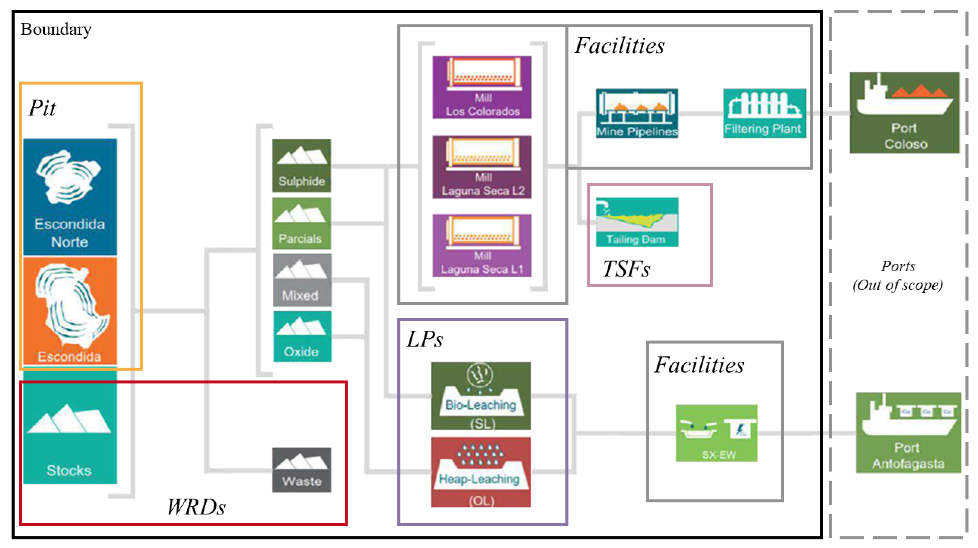
2.2. Scope and Feature Distinction

Based on the reasons described in Section 1, we focused on copper mines in Chile. Filtering the data from S&P Capital IQ Pro (hereafter SNP, a comprehensive financial data and analytics platform for mining professionals, investors, and analysts) [50] according to mining methods, commodities, and reported copper production quantities in 2021, we selected 15 open-pit sites with copper as the primary commodity (Figure 1a, see

Table A3. Information for each copper mine and satellite images used in this study.

Mine Site	Start Year	Stage	Commodities	Method	Image Date	Satellite Series	Sensor
Escondida	1990	Operating	Cu, Au, Ag	Open Pit	1989.05.20 1995.01.05 2000.02.12 2005.01.16 2010.01.14 2015.04.02 2020.03.30	Landsat 4–5 Landsat 4–5 Landsat 4–5 Landsat 4–5 Landsat 4–5 Landsat 8–9 Landsat 8–9	TM TM TM TM TM OLI/TIRS OLI/TIRS
Collahuasi	1999	Expansion	Cu, Mo, Ag, Au	Open Pit	1999.04.13 2005.03.12 2010.04.11 2015.02.20 2020.02.02	Landsat 4–5 Landsat 4–5 Landsat 4–5 Landsat 8–9 Landsat 8–9	TM TM TM OLI/TIRS OLI/TIRS
Radomiro Tomic	1997	Operating	Cu, Mo	Open Pit	1997.12.19 2000.11.25 2005.11.23 2010.12.07 2015.12.21 2020.12.18	Landsat 4–5 Landsat 4–5 Landsat 4–5 Landsat 4–5 Landsat 8–9 Landsat 8–9	TM TM TM TM OLI/TIRS OLI/TIRS
Los Pelambres	1999	Expansion	Cu, Mo, Au, Ag	Open Pit Underground	1995.12.07 2001.02.06 2005.03.05 2010.12.16 2015.12.14 2020.12.27	Landsat 4–5 Landsat 4–5 Landsat 4–5 Landsat 4–5 Landsat 8–9 Landsat 8–9	TM TM TM TM OLI/TIRS OLI/TIRS
Sierra Gorda	2015	Operating	Cu, Mo, Au, Ag	Open Pit	2014.12.02 2016.12.23 2018.12.13 2020.12.02	Landsat 8–9 Landsat 8–9 Landsat 8–9 Landsat 8–9	OLI/TIRS OLI/TIRS OLI/TIRS OLI/TIRS
Centinela Sulfide	2011	Operating	Cu, Au, Ag, Mo	Open Pit	2011.10.23 2015.12.21 2020.12.02	Landsat 4–5 Landsat 8–9 Landsat 8–9	TM OLI/TIRS OLI/TIRS
Ministro Hales	2010	Operating	Cu, Ag, Mo, Au	Open Pit Underground	2010.12.07 2013.12.31 2015.12.21 2017.12.26 2020.12.18	Landsat 8–9 Landsat 8–9 Landsat 8–9 Landsat 8–9 Landsat 8–9	OLI/TIRS OLI/TIRS OLI/TIRS OLI/TIRS OLI/TIRS
Candelaria	1994	Operating	Cu, Au, Ag, Fe	Open Pit	1995.07.23 2000.10.24 2005.09.04 2010.11.21 2015.11.19 2020.08.28	Landsat 4–5 Landsat 4–5 Landsat 4–5 Landsat 4–5 Landsat 8–9 Landsat 8–9	TM TM TM TM OLI/TIRS OLI/TIRS
Spence	2006	Expansion	Cu, Ag, Mo, Au	Open Pit	2006.12.28 2010.12.07 2015.12.21 2020.12.02	Landsat 4–5 Landsat 4–5 Landsat 8–9 Landsat 8–9	TM TM OLI/TIRS OLI/TIRS
Caserones	2013	Operating	Cu, Mo	Open Pit	2013.11.22 2015.12.30 2017.12.03 2020.12.27	Landsat 8–9 Landsat 8–9 Landsat 8–9 Landsat 8–9	OLI/TIRS OLI/TIRS OLI/TIRS OLI/TIRS
Gabriela Mistral	2008	Operating	Cu, Mo	Open Pit	2008.12.26 2010.12.16 2015.12.30 2020.12.11	Landsat 4–5 Landsat 4–5 Landsat 8–9 Landsat 8–9	TM TM OLI/TIRS OLI/TIRS
Zaldivar	1995	Operating	Cu	Open Pit	1995.01.05 2000.02.12 2005.01.16 2010.01.14 2015.04.02 2020.03.30	Landsat 4–5 Landsat 4–5 Landsat 4–5 Landsat 4–5 Landsat 8–9 Landsat 8–9	TM TM TM TM OLI/TIRS OLI/TIRS
Centinela Oxide	2001	Operating	Cu, Mo, Au	Open Pit	2001.12.30 2005.11.23 2010.12.07 2015.12.21 2020.12.02	Landsat 4–5 Landsat 4–5 Landsat 4–5 Landsat 8–9 Landsat 8–9	TM TM TM OLI/TIRS OLI/TIRS
Antucoya	2015	Operating	Cu	Open Pit	2015.12.21 2017.12.26 2020.12.02	Landsat 8–9 Landsat 8–9 Landsat 8–9	OLI/TIRS OLI/TIRS OLI/TIRS
El Abra	1996	Operating	Cu, Au, Mo, Ag	Open Pit	1996.12.16 2000.11.25 2005.11.23 2010.12.07 2015.12.21 2020.12.02	Landsat 4–5 Landsat 4–5 Landsat 4–5 Landsat 4–5 Landsat 8–9 Landsat 8–9	TM TM TM TM OLI/TIRS OLI/TIRS

in Appendix C for details). The selected mines are all located in northern Chile, corresponding to the two northernmost regions in the natural regions classification—Norte Grande (Far North or Great North) and Norte Chico (Near North). Most of the mines are situated at altitudes ranging between 2000 and 4000 m. In 2021, the 15 sites produced 86.3% of Chile’s total copper production and accounted for 79.8% of the total estimated reserves in Chile.

We distinguished six features of copper mine sites: pit, WRDs, LPs, facilities, TSFs, and others (Figure 1b). Features were distinguished based on expert judgment, maps in technical reports (

Table A2. References used for mapping each of the mines.

Mine Site	References
Escondida	Basto [130]: Slide 12, 15, 25, 26, and 28; BHP [58]: Figures 13–16, 15-2, and 15-7.
Collahuasi	Map tool from Mapcarta [131]; Description text from Mining Technology [132].
Radomiro Tomic	Calderón D. et al. [133]: Figure 2 on page 6, and other in the report; Figures on page 4 and 5.
Los Pelambres	-
Sierra Gorda	Lopez and Ristorcelli [134]: Figures 5-5, 23-9, and 23-15.
Centinela Sulfide	Antofagasta plc. [135]: Figures on page 6, 10, 19, and 29.
Ministro Hales	Knight Piésold [136]: Figures 2.2-2, 2.2-3, 2.2-4, and 3.1-1; Boric et al. [137]: Figures 1 and 2a; Campos P. [138]: pages 2 and 9.
Candelaria	Lundin mining [139]: Figures on pages 19, 23, 31, 67, 68, and 73.
Spence	BHP Billiton [140]: Figures of project layout on pages 2 and 3; BHP Billiton [141]: Figures on page 25, 31, and 49.
Caserones	Walker [142]: Figures 4.2, 4.5, 5.3, and 5.4.
Gabriela Mistral	-
Zaldivar	Evans and Lambert [59]: Figures 4-2, 4-3, and 18-1.
Centinela Oxide	Antofagasta plc. [135]: Figures on pages 6, 10, 19, and 29.
Antucoya	-
El Abra	Adkerson et al. [143]: Description text on pages 14 and 25, as well as other pages.

), the logic of copper mining and refining (Figure A1), and potential environmental risks. Details of definitions, identification methods, and specific examples for each feature are summarized in Appendix B.

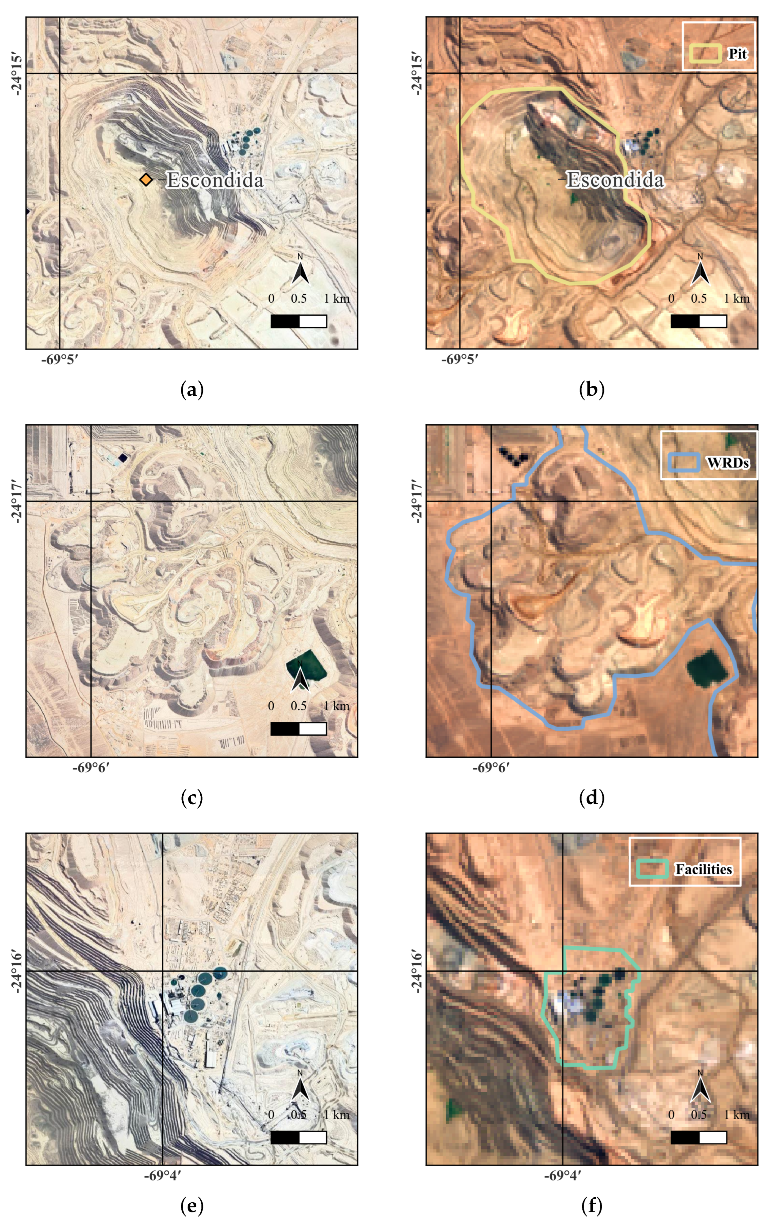
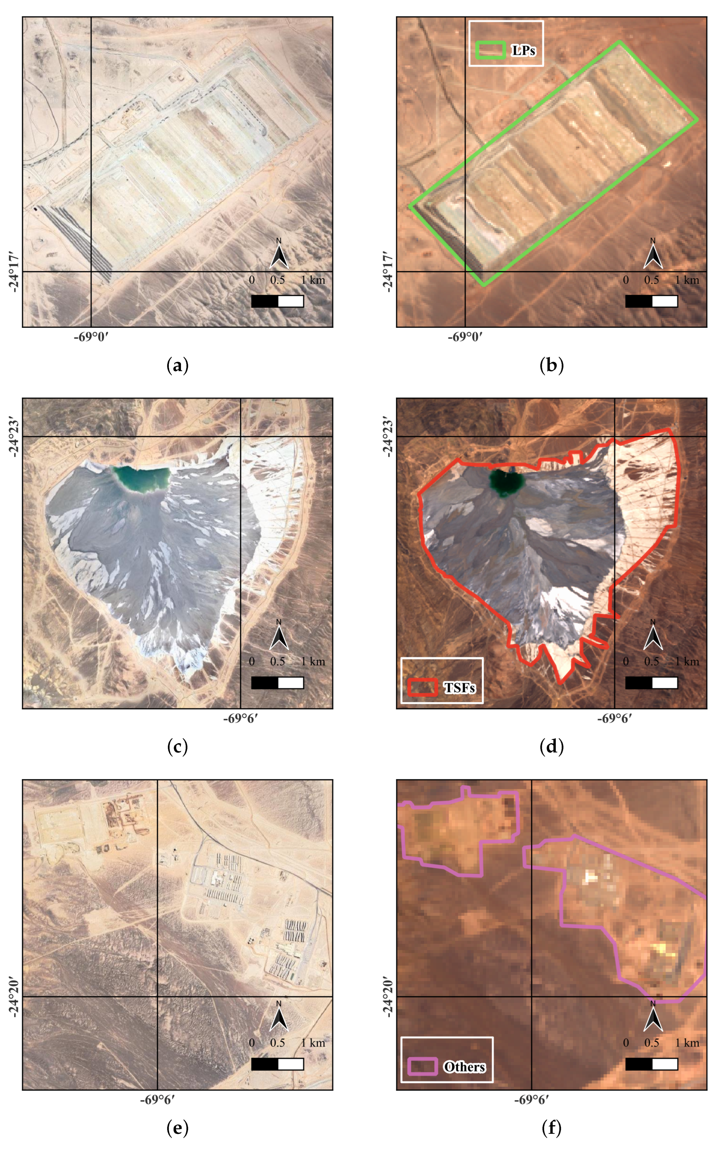
2.3. Mapping Using Satellite Imagery and GIS

The method used for satellite image analysis in this study is based on the “Geographically explicit land-use mapping” approach described in [22] (Chapter 2). Considering the long timespan of observation and data consistency, we used satellite images from the Landsat series, which started recording images in 1972 [51].

Satellite images were downloaded from the Global Visualization Viewer (GloVis, USA), an online search and ordering tool provided by U.S. Geological Survey [52]. Compared to past studies that have selected several specific periods without the start year of mining projects (e.g., [37]), we observed successive land occupations since each mining project started, with 2- to 5-year intervals (see Table A3 in Appendix C), to track land occupation and transformation through the history of each mine site.

Satellite images underwent band composition using Python (3.11.2) with open-source libraries gdal [53]. A polygon delineation of features was then conducted through visual interpretation using open-source GIS software QGIS (3.38.2-Grenoble, QGIS.ORG, Switzerland) [54]. Because of the resolution of the satellite images from Landsat (30 m), and to increase the accuracy of delineation, we georeferenced very-high-resolution Google Earth images and site-planning maps in technical reports from mining companies (see Table A2) in QGIS as a reference. Data from OpenStreetMap (OSM) [55], including point, line, and polygon layers, and interpretations from experienced mining experts were also involved for the further validation of the mapping results.

2.4. Data Analysis

We analyzed the mapping data in two main steps: area calculation and analysis combined with operational data. The area of each polygon was calculated using the geopandas [56] Python package under the reprojected coordinate reference system WGS 84/UTM, zone 19S (EPSG:32719), which is suitable for area calculations between ${72}^{\circ }$ W and ${66}^{\circ }$ W in the Southern Hemisphere [57]. The total occupied area ($A_T$) of a mine (m) in a year (t) is calculated using Equation (2). In addition, because we delineated the polygons of each feature, the proportion ($por$) that each feature (i) occupies in the total area in year (t)—for understanding the spatial composition of each mine—was calculated and compared among sites using Equation (3).

$$\begin{array}{cc}\hfill A_{T,m,t}& =A_{Pit,m,t}+A_{WRDs,m,t}+A_{TSFs,m,t}+A_{Facilities,m,t}+A_{LPs,m,t}+A_{Others,m,t}\hfill \end{array}$$

(2)

$$\begin{array}{cc}\hfill po{r}_{i,m,t}& ={\displaystyle \frac{A_{i,m,t}}{A_{T,m,t}}}\times 100\%\hfill \end{array}$$

(3)

Next, to analyze the relationship between occupied land and factors in mining activity, we combined area data with operational data obtained from the SNP database [50], including the coordinates of mines, commodities, mining methods, and the annual production of ore, copper, and waste.

The LTF, a parameter indicating the area of land occupied (m²) for producing a unit (kg) of target materials (in this study, copper), was calculated using Equation (4). The LTF shows the relationship between the occupied land area ($A_{T,m,t}$) and the cumulative material production (P) within the period ($[t_0,t]$). The LTF was analyzed and compared with other similar factors in other research, such as weighted disturbance rates (WDRs) in [34]. We distinguished three different LTFs, $LT{F}_{Ore}$, $LT{F}_{Copper}$, and $LT{F}_{Waste}$, which were calculated using Equations (5), (6), and (7), respectively.

$$\begin{array}{cc}\hfill & LT{F}_{m,t}={\displaystyle \frac{A_{T,m,t}}{{\sum }_{t_0}^t{P}_t}}\hfill \end{array}$$

(4)

$$\begin{array}{cc}\hfill & LT{F}_{Ore,m,t}={\displaystyle \frac{A_{T,m,t}}{{\sum }_{t_0}^t{P}_{Ore,t}}}\hfill \end{array}$$

(5)

$$\begin{array}{cc}\hfill & LT{F}_{Copper,m,t}={\displaystyle \frac{A_{T,m,t}}{{\sum }_{t_0}^t{P}_{Copper,t}}}\hfill \end{array}$$

(6)

$$\begin{array}{cc}\hfill & LT{F}_{Waste,m,t}={\displaystyle \frac{A_{WRDs,m,t}+A_{TSFs,m,t}}{{\sum }_{t_0}^t(P_{Ore,t}+P_{Waste,t}-P_{Copper,t})}}\hfill \end{array}$$

(7)

3. Results

3.1. Site-Specific Mapping and Feature Composition Analysis

As shown in Figure 2, 2026 polygons were delineated, based on 62 satellite images covering the lifespan of 15 mines between 1989 and 2020, with intervals ranging from 2 to 5 years (see Table A3). The land occupation results (Figure 3) of three representative mines with relatively long operation period since the 1990s—Escondida, Zaldivar, and Los Pelambres—were compared to assess the different characteristics of the mines.

Figure 3a,b illustrates temporal changes in land occupation and feature composition of Escondida and Zaldivar, respectively. Two mines are closely situated (Figure 2a) and commenced operation at a similar time (1989 and 1995). In 1989, Escondida started its operation with the gradual expansion of WRDs, and subsequently, the area of pit and TSFs became larger. TSFs overtook WRDs and became the largest feature in 2005, due to the start-up of the Escondida Norte Mine in 2005 with the construction and expansion of the Escondida Norte open pit and Laguna Seca TSF in the southern part of the mine [58]. Until 2020, waste storage facilities (WSFs)—WRDs (28%) and TSFs (41%)—accounted for 69% of the total area (149.48 km²), whereas pits accounted for only 8%. In comparison, the change in proportion of each feature was not obvious in Zaldivar since it started in 1995 and continued till 2020, with WSFs (WRDs: 41% > TSFs: 25%) accounting for 66% of total land occupation (23.75 km²) and pits accounting for 15%. This result reveals that a significant proportion of space was occupied by WSFs within mining areas, consistent with the findings of [18]. This reinforces the significant attention paid to the management of WSFs at mine sites.

Our results highlight the influence of mine-site processing methods on land transformations. For example, it is notable that the proportions of WRDs and TSFs are starkly different between Escondida and Zaldivar. This is largely attributable to the use of dump and heap leaching at Zaldivar [59], with waste material stacked in TSFs in solid form. In contrast, Escondida employs both leaching and froth flotation in its processing method. The froth flotation method generates a large amount of tailings, requiring the construction of a large-scale tailings dam for storage and thereby significantly increasing the proportion of WSFs in the occupied land of the mine. This heterogeneity highlights the need for a more site-specific mapping and characterization of mine sites to obtain a deeper understanding of site-specific characteristics.

A comparison of the chronological land occupation map in Figure 3a–c reveals differences in the spatial distribution of features among three mines. From the maps of Escondida and Zaldivar, it is evident that all features exhibit a concentrated distribution within the depicted space. This configuration of features can be characterized as a “dense type”, which is often observed in mines situated on flat terrain that permits site operations immediately adjacent to orebodies. This distribution concentrates the features and reduces transportation time and costs, thereby enhancing economic efficiency. Correspondingly, the “dispersed type” is exemplified in areas such as the Los Pelambres mining district, where features exhibit irregular distribution and may display noticeable and sizable gaps between them. This is often attributed to the physical spatial constraints imposed by the terrain, such as mountain ranges or valleys (see Figure 4c). While the dispersed-type distribution tends to have smaller total land occupation (e.g., Los Pelambres: 20.63 km² in 2020), the influence of topographical factors suggests that unexpected incidents (e.g., earthquakes) may lead to more severe losses, and indeed, the total area in which mining is the dominant land use increases. Therefore, the analysis of MLT should not only consider the size of land occupation but also require a thorough understanding of the topography and spatial distribution of features.

3.2. Assessing Land Transformation Versus Mining Activity

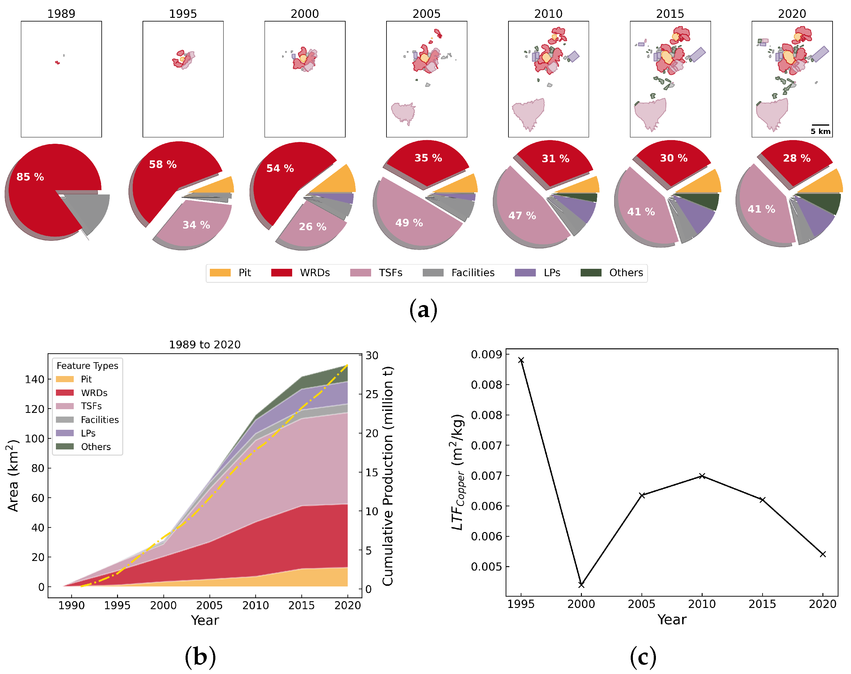
3.2.1. Temporal Changes in Copper Production and Land Transformation

The relationship between the total occupied area and cumulative production until 2020, and the relationship between the area for WSFs (including WRDs and TSFs) and total waste production, are plotted in Figure 4a and Figure 4b, respectively. Both figures exhibit an approximately linear relationship. The slopes of the fitted lines, referring to LTF_Copper and LTF_Waste in 2020, were 0.0045 m²/kg and 9.87 × 10⁻⁶ m²/kg. Despite high correlation coefficients (r = 0.94 and r = 0.90, respectively), these linear fitted results are not ideal for direct application to LCA inventories. This is primarily due to (1) some sites diverging greatly from the fitted lines and (2) these values being specific to the selected 15 mines for the year 2020 only. Therefore, we conducted a more comprehensive temporal investigation of land transformation and production.

Figure 4c–f show the chronological changes in the occupied area and the cumulative production data of four sample mine sites, which were all in the operation stage in 2020 (see Table A3 in Appendix C). Except for Radomiro Tomic, which has no available production data from 2005 to 2007 from either [50] or [60], cumulative production shows nearly linear growth because each mine tends to maintain the continuous operation of the production line and a stable supply to the market. In contrast, changes in land varied between sites, with a tendency to gradually stabilize over time. For Radomiro Tomic and Ministro Hales, the occupied area expanded gradually and linearly; however, for Escondida and Zaldivar, several turning points can be seen due to periods of project expansion. Let us take Escondida (Figure 4c) as an example. The areas of TSFs and WRDs increased rapidly after 2000 due to the start-up of the Phase 4 Escondida expansion (Laguna Seca tailings dam) in 2002, and LPs expanded after 2010 following the announcement of the Oxide Leach Area Project (OLAP) [58]. This indicates that, while the production volumes of mines do not exhibit significant annual variations, the relationship between land transformation and production may change because of factors such as mine development plans. Therefore, using production volumes to calculate land transformation areas retroactively can lead to significant inaccuracies.

3.2.2. Comparative Analysis of LTFs

$LT{F}_{Copper}$ was calculated per Equation (6) and plotted in Figure 5a. It illustrates that, for the 15 mines selected in this study, each mine exhibited a trend in which the $LT{F}_{Copper}$ was relatively high during the initial stages and gradually decreased over the life of the project. This trend aligns with that found in Ni mines by [37]. In addition, the results indicate significant variability in the $LT{F}_{Copper}$ during the initial stages of each mine, followed by a gradual decrease as mining progresses. However, the logarithmic graph further illustrates that, although the LTF values are minimal in 2020, substantial differences persist between the mines.

To further investigate the factors that may influence LTFs, an analysis of snapshots in 2020 is plotted in Figure 5b–e. In the context of mining activities, gold (Au), a high-value byproduct, may influence mining operations. However, our data indicate that the presence of gold in commodities does not significantly affect LTFs. This is consistent with the findings of [38], who found that commodity types did not statistically influence land transformation.

Figure 5b and Figure 5c respectively represent the numerator and denominator of the LTF formula. There is no clear relationship between the area and LTF. In contrast, the cumulative production shows a more pronounced regularity in its influence on LTF, with LTF significantly decreasing as the cumulative production increases.

Figure 5d illustrates that the size of the transformed land area was not strongly correlated with the duration of mining activity. This is because (1) the scale of mining operations can be influenced by various social factors, such as permits from the government, resource reserves, financial investment, and mining methods, and (2) there is a slowdown in horizontal expansion. In the early stages of mine development, rapid expansion can be seen from the satellite images for Pit and WRDs in particular; however, the expansion slows down because of the vertical pile-up of waste and deep digging into the pit. Therefore, a longer duration of mining development does not necessarily imply a continued rates of expansion. Figure 5e illustrates a clear decreasing trend in LTF as the duration of mining projects increases. As analyzed in Section 3.2.1, with the progression of the mining project duration, cumulative production volumes show a linear increase, whereas the area of land occupation tends to stabilize, ultimately resulting in a reduction in $LT{F}_{Copper}$ over time.

3.2.3. The Variations and Disparities in LTFs

In addition to $LT{F}_{Copper}$, $LT{F}_{Ore}$ and $LT{F}_{Waste}$ were calculated and plotted in Figure 6 (detailed data provided in

Table A4. Chronological land transformation factor for 15 mines.

Sitename	Year	Area (km2)	LTFOre (m2/kg)	LTFCopper (m2/kg)	LTFWaste (m2/kg)
Escondida	1989 1995 2000 2005 2010 2015 2020	0.50 16.63 31.13 71.89 115.74 141.66 149.61	inf 0.000208 0.000109 0.000117 0.000112 0.000101 0.000076	inf 0.008404 0.004696 0.006173 0.006492 0.006101 0.005204	inf 0.000024 0.000013 0.000018 0.000017 0.000014 0.000012
Average			0.000121	0.006178	0.000016
Collahuasi	1998 2005 2010 2015 2020	10.85 28.37 44.45 54.81 58.11	0.001072 0.000097 0.000069 0.000055 0.000043	0.226019 0.009265 0.008142 0.007246 0.005615	0.000139 0.000018 0.000014 0.000011 0.000009
Average			0.000267	0.051257	0.000038
Radomiro Tomic	1997 2000 2005 2010 2015 2020	5.13 11.66 18.42 28.43 36.24 42.82	0.005169 0.000115 0.000047 0.000041 0.000036 0.000034	1.266449 0.021305 0.011387 0.010800 0.007961 0.007078	0.001115 0.000031 0.000014 0.000012 0.000011 0.000009
Average			0.000907	0.220830	0.000199
Los Pelambres	1995 2000 2005 2010 2015 2020	1.27 7.45 12.03 16.50 18.27 20.63	inf 0.000183 0.000047 0.000033 0.000022 0.000018	inf 0.024916 0.006022 0.004524 0.003249 0.002788	inf 0.000049 0.000011 0.000007 0.000004 0.000003
Average			0.000061	0.008300	0.000015
Sierra Gorda	2014 2016 2018 2020	12.98 30.20 35.07 38.08	inf 0.000533 0.000262 0.000172	1.180215 0.159857 0.091603 0.059516	-0.687322 0.000070 0.000037 0.000026
Average			0.000322	0.372798	0.000044
Centinela Sulfide	2011 2014 2016 2018 2020	13.50 18.03 28.13 30.67 36.15	0.000536 0.000132 0.000140 0.000115 0.000108	0.149785 0.029999 0.030356 0.024615 0.022665	0.000088 0.000020 0.000022 0.000018 0.000017
Average			0.000206	0.051484	0.000033
Ministro Hales	2013 2015 2017 2020	9.19 11.06 11.99 14.63	0.005103 0.000336 0.000154 0.000106	0.273606 0.026779 0.013856 0.010578	0.000068 0.000031 0.000019 0.000012
Average			0.001425	0.081205	0.000032
Candelaria	1994 2000 2005 2010 2015 2020	1.29 8.39 10.98 13.50 15.80 23.14	0.000530 0.000084 0.000049 0.000038 0.000031 0.000036	0.046087 0.007379 0.005120 0.004418 0.004044 0.004958	0.000047 0.000012 0.000008 0.000005 0.000005 0.000006
Average			0.000128	0.012001	0.000014
Spence	2007 2010 2015 2020	12.49 16.94 26.27 34.21	inf inf inf inf	0.165475 0.030777 0.018823 0.014832	−0.066392 −0.013349 −0.010458 −0.008994
Average			nan	0.057477	nan
Caserones	2013 2015 2017 2020	4.01 5.76 7.47 9.90	inf 0.000083 0.000045 0.000031	0.247678 0.041774 0.019867 0.012599	−0.112732 0.000029 0.000019 0.000014
Average			0.000053	0.080479	0.000021
Gabriela Mistral	2008 2010 2015 2020	5.45 9.30 14.75 18.08	0.000354 0.000149 0.000065 0.000043	0.080508 0.027952 0.015395 0.011928	0.000105 0.000050 0.000021 0.000016
Average			0.000153	0.033946	0.000048
Zaldivar	1995 2000 2005 2010 2015 2020	1.95 12.02 15.24 17.49 22.31 23.75	0.000830 0.000139 0.000089 0.000065 0.000055 0.000043	0.097963 0.019182 0.011531 0.008661 0.008536 0.007593	0.000081 0.000018 0.000015 0.000011 0.000011 0.000009
Average			0.000203	0.025578	0.000024
Centinela Oxide	2001 2005 2010 2015 2020	2.96 6.56 13.33 18.16 19.62	0.000667 0.000164 0.000144 0.000133 0.000094	0.068823 0.015794 0.015169 0.013422 0.011336	0.000091 0.000022 0.000017 0.000015 0.000010
Average			0.000241	0.024909	0.000031
Antucoya	2015 2017 2020	4.79 10.19 14.48	inf 0.000217 0.000110	0.392442 0.064117 0.037881	−0.143797 0.000066 0.000035
Average			0.000164	0.164813	0.000050
El Abra	1996 2000 2005 2010 2015 2020	4.62 7.87 11.51 21.05 22.99 24.37	0.001697 0.000049 0.000023 0.000028 0.000024 0.000022	0.247293 0.009208 0.005827 0.007430 0.006421 0.006088	0.000604 0.000021 0.000012 0.000016 0.000012 0.000010
Average			0.000307	0.047045	0.000112

in Appendix E). Similar to $LT{F}_{Copper}$, $LT{F}_{Ore}$ and $LT{F}_{Waste}$ exhibit a trend of a gradual decrease with an increasing duration of mining activity, for reasons similar to those mentioned in Section 3.2.2. However, the difference in the volume of ore/waste and copper results in a difference in the magnitude of $LT{F}_{Ore}$ and $LT{F}_{Copper}$, indicating the necessity to declare a clear definition of each factor, as well as a formula for calculation, if used.

Comparing the average values of LTF_Copper among the mines reveals a two-digit difference between the maximum value of 0.372798 m²/kg (Sierra Gorda) and the minimum of 0.006178 m²/kg (Escondida). Such a difference can also be observed in LTF_Ore and LTF_Waste, indicating that using average values to represent the conditions of all mining areas can lead to significant uncertainty, potentially conveying inaccurate information to the public or even guiding policymakers to formulate inappropriate policies (e.g., if permits are granted on the assumption that a region will be developed to a certain extent).

In addition, LTF_Ore values in Table A4 in Appendix E were compared with factors from two sources: (1) the mean value in ecoinvent for “land transformation from nature to mine” during the “Mining copper ore, GLO; mining” process (6.25 × 10⁻⁵ m²/kg-Ore) and (2) the weighted disturbance rates (WDRs) of copper (4.5 ha/Mt-Ore, 4.5 × 10⁻⁵ m²/kg-Ore) calculated by [34], which was defined as the ratio of the annual quantity of area (ha) newly disturbed and ore extracted (million metric tons). The LTF_Ore of Mine Caserones (5.3 × 10⁻⁵ m²/kg-Ore), which was the lowest average value of LTF_Ore in this study, was the closest value to these averages of copper. This suggests that, if the results in [33,34] were applied to describe the 15 mine sites in this study, the results of the area calculation—the basis of further assessment—would be underestimated.

4. Discussion

4.1. On the Importance and Benefits of Spatial Data

Compared to other inventories in LCA, such as the energy consumption and global warming potential (GWP, unit: kg CO₂ eq) of a specific material, which are relatively easy to quantify, land is a much more complex issue. Land cover is the result of the combined effect of large spatial variations in a number of natural elements, including geomorphology, geology, and hydrology. At the same time, changes on land can be the root cause of numerous environmental impacts and even disasters, such as soil degradation, localized earthquakes, and landslides.

Current LCA studies evaluate land-related aspects, such as the potential damage (D, see Equation (8)), using the occupied area (a) affected from the initial stage ($t_0$) to a specific stage (t) as a key metric for the characterisation factor—ecosystem damage potential (EDP) [28]. Models for calculating mining areas have been proposed and used in LCA [35,37,61]. Although clearly important, land area should not be the only aspect considered. The simplification of “land” into “area” may result in the nuance of spatial distribution and arrangement being overlooked, which is important for environmental assessment and risk evaluation.

$$\begin{array}{c}\hfill D={\int }_0^a{\int }_{t_0}^{t}EDP(a,t)·\mathrm{d}a\mathrm{d}t\end{array}$$

(8)

Accordingly, our results strongly suggest that any assessment related to land in LCA should incorporate geographic data where possible to fill the gap raised by [62]. A synthesized GIS database on mining could be constructed to support this, as was also suggested in [30,63]. In lieu of public reporting, our remote sensing satellite imagery and GIS approach offer the possibility of obtaining independent data on spatiotemporal changes in mines at a low cost. The benefits of creating a GIS database for mines include but are not limited to the following:

1.

Enabling a combination of temporally georeferenced attribute data. In this study, we combined GIS polygons and operational data to calculate the temporal land transformation factor site-specifically. Attribute data, such as locally measured data on water contamination, soil properties, population density, and economic data, if available, can also be supplemented and integrated for a more comprehensive analysis.

2.

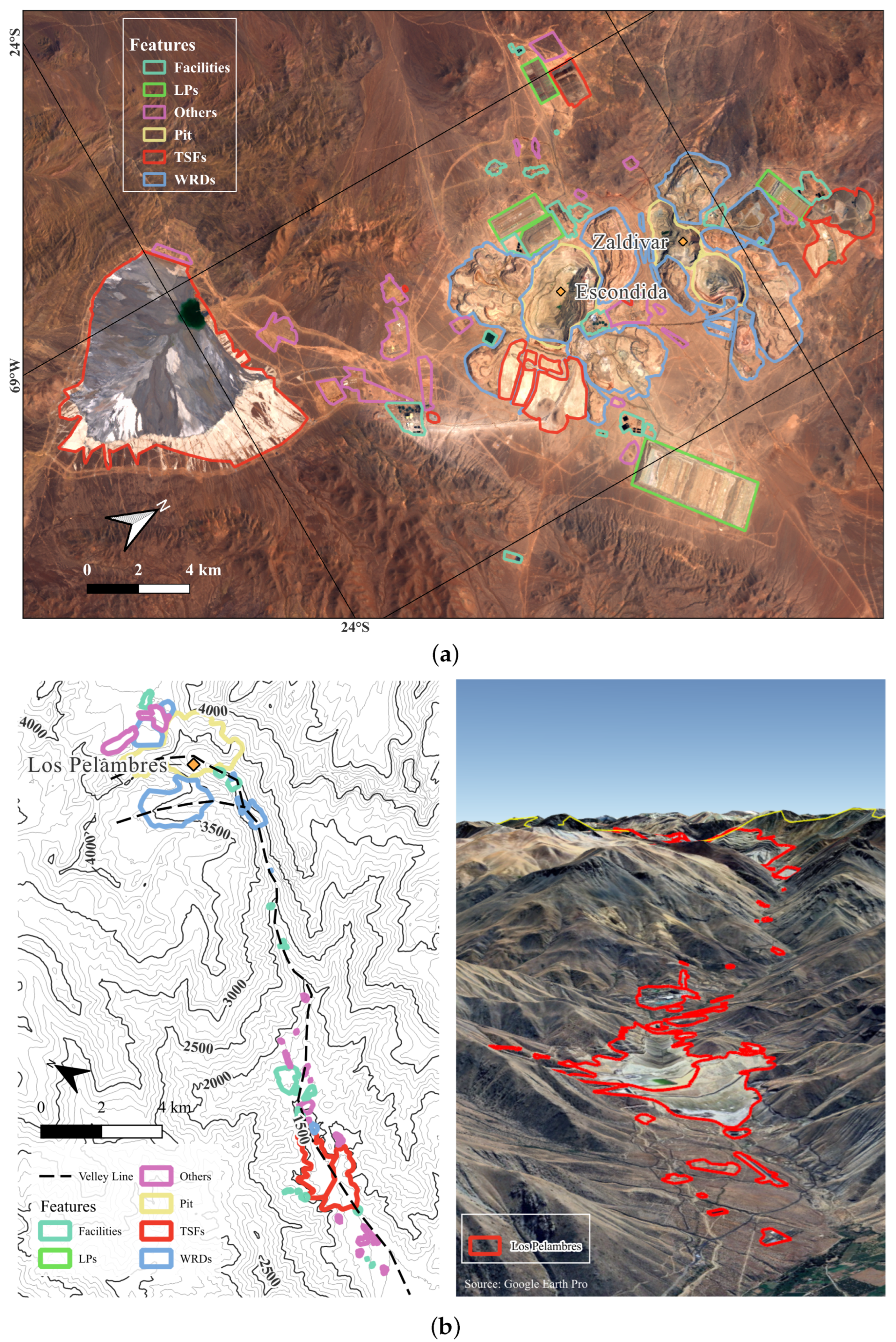
The visualization of land occupation/transformation can easily be achieved in the form of maps. The process of land transformation is illustrated in Figure 3, which can be used to improve the basis for decision-making in industry and other organizations.

3.

Integrated spatial analysis can be conducted by overlaying it with other types of maps (e.g., geological, water system, and urban planning maps) to improve the accuracy [28] and reliability of the environmental evaluation and risk assessment of mining projects.

In this study, we provide a basic sample of geographic data and part of its application methodologies. The obtained data can not only be used in coupling with production data to calculate the LTF required for LCA but also have direct applications in multiple disciplines related to mining, such as industrial ecology, environmental, and disaster science. Biodiversity assessment, water pollution range prediction, and potential disaster prediction can be implemented based on these geographic data. Additionally, field sampling data (e.g., water and soil samples) can be integrated as attribute data to create a more comprehensive information model for LCA and environmental assessment to enhance sustainable resource development and cleaner production in a mining context.

4.2. On the Reconsideration of Land-Related Factors in LCA

As mentioned in [35], in LCA, “the environmental impact of mining can be calculated by multiplying the land transformation area per unit of ore mined by the impact on the ecosystem per unit of area changed”. However, it should be noted that the LTF does not represent the causal relationship between production and land transformation/occupation because of the lack of objective physical principles. As defined by Equation (4), LTF is calculated based on area and production, indicating the area of land occupied for production per unit of target products, which is a quantitative indicator of the efficiency of occupied land utilization, not of the causal relationship between them, and can be affected by a combination of both natural and anthropogenic factors. Therefore, the suitability and applicability of LTF for land-related calculations (e.g., environmental impacts or biodiversity loss) for mining need to be discussed and verified.

Additionally, among the 15 mine sites in 2020, the average value of $LT{F}_{Copper}$ (0.0148 m²/kg-Cu), the median value (0.0106 m²/kg-Cu), and the slope of the fitted line in Figure 4a (0.0045 m²/kg-Cu) showed significant differences, and no evidence could be found regarding which of these values can better represent these 15 mines. When accounting for each individual mine or different time periods, the variability in the results becomes significantly greater, rendering it impractical to select a single value that accurately represents the overall scenario. The results in Section 3.2.2 and Section 3.2.3 demonstrate that utilizing a single value to represent different mines and over different time periods is insufficient.

While our study enables accurate LTF calculations for the mines assessed, the sheer work required to gather production and spatial data for the world’s mines remains enormous. Work is ongoing to compile production data (e.g., [64,65]), and footprint data (e.g., [2,38,39]) at global scales that will help to enable these efforts; however, integrating these datasets also remains a major challenge. In the meantime, it is clear that the uncertainties associated with land transformation data (e.g., ecoinvent [33]) per current LCA methods are high. Our study emphasizes that such uncertainties ought to be clearly acknowledged.

Compared to estimating MLT areas based on production data and LTF, or using nation-/region-wide averages to represent the situation of all mines in a specific region, maps generated from satellite imagery and GIS data in this study provide a more accurate and realistic reflection of land transformation. These geospatial techniques offer precise, site-specific insights into how mining activities directly alter the landscape, capturing the variability between individual sites and their unique environmental impacts.

4.3. Recommendations for Sustainable and Responsible Mining

Land is an important resource, and any modification of land in the course of industrial production like mining entails an occupation and destruction of native land resources, which, in turn, causes direct or indirect damage to the surrounding ecological environment. In the context of sustainable development and cleaner production, land reclamation and rehabilitation, soil remediation, and ecosystem restoration in mining areas have become pressing issues [66]. Ideally, governments and companies that profit from mining activities are obligated to restore the land to its original state prior to extraction. However, only a handful of post-mining area have been reclaimed [67,68], and the rest became “mining legacies” with long-term environmental effects. The 15 mines examined in this study, regardless of the duration of their operation, all showed continuous land expansion, likely because they are still in active production. However, in the coming decades, as copper resources are depleted, it remains uncertain whether these lands will be reclaimed or become new “mining legacies” and what environmental consequences may follow. To avoid tragedies like those summarized by [15] in the history of Chile, and to promote sustainable mining practices, here, we propose recommendations based on the methods and findings of this study.

4.3.1. Waste Management

Based on our analysis of feature composition in Section 3.1, WSFs—TSFs and WRDs—occupy more than half of the land area in each mine, and these facilities pose the greatest environmental risks. Therefore, every mining company should ensure the following:

1.

During the detection and planning phase, in addition to selecting appropriate locations and construction methods for all facilities, post-closure rehabilitation measures should also be planned properly.

2.

During the operational phase, these facilities must be properly managed to minimize pollution and prevent potential disasters like tailings dams’ failure.

3.

During the post-mining phase, these facilities should be subject to long-term monitoring, and the land should be gradually reclaimed and rehabilitated to minimize the environmental impacts and associated risks.

Although land reclamation and rehabilitation are known to be costly (250–400 Euro/m² for land reclamation, according to [66]), in the context of sustainable development, the ability to rehabilitate land at a reasonable cost will become both an opportunity and a challenge for mining companies. Furthermore, governments should strictly assess the clarity and feasibility of rehabilitation plans, particularly for high-risk land areas like waste storage facilities, when granting mining permits.

4.3.2. Public Attention and Information Disclosure

In the broader context of climate change and the Sustainable Development Goals (SDGs), much of the focus has been on carbon emissions and new energy technologies [69]. In contrast, land issues, particularly those related to mining activities in remote regions, receive far less attention [20,70]. As [71] pointed out, greater attention needs to be paid to public participation and justice concerns associated with mine sites. However, the lack of information disclosure serves as a significant barrier to public participation. Through the investigation in this study, we found it challenging to obtain information on land transformation related to mining activities. Among the 15 mines studied, we could not locate any directly usable geographic data disclosed by the companies. Instead, only reference maps were found in the reports of 12 mines, as listed in Table A2 in Appendix B. This indicates that, compared to the progress made in disclosing information related to carbon emissions, minimal advancement can be seen in disclosure of land transformation information by governments or companies.

Based on the reports summarized in Table A2 and the knowledge of the mining industry, it is evident that mining companies possess extensive geographic data that could be used to create maps. However, why have they not made these information publicly available? Three possible reasons can be raised: (1) they are not required to disclose such information; (2) they are uncertain about what type of data to release and in what format; (3) concerns over liability. These reasons highlight significant policy deficiencies, particularly the lack of mandatory regulations, and clear guidelines and instructions regarding the disclosure of land-related information. To address these issues, we propose recommendations from two perspectives.

Policy-wise, governments should introduce regulations that require mining companies to disclose geographic data related to MLT, including waste storage facilities and mining areas, with clear guidelines on what specific data needs to be made public (e.g., spatial data on land use and environmental impacts) and in which formats. These regulations should enforce the release of standardized, GIS-compatible datasets that allow for easy tracking and monitoring by the public and researchers. Incentives (e.g., tax benefits) can be provided for companies that go beyond compliance in information transparency, encouraging voluntary data sharing as part of corporate social responsibility.

On the other hand, before policies are improved, the public can use the methods developed in this study to monitor and track MLT independently. By utilizing open-source remote sensing and GIS techniques, individuals or communities can build GIS databases to monitor MLT in mining regions. This would provide a valuable resource for both advocacy and policy-making, and it would allow for more informed public participation in environmental governance and sustainable production.

4.4. Uncertainties and Limitations

Uncertainties in this study arise from the quality and incompleteness of the source data. Open-source satellite imagery from Landsat (30 m) made it difficult to define the exact boundary of features more precisely; therefore, the measured area may slightly differ from actual values. In addition, owing to the long-range capture of satellite imagery, shadows due to altitude and image distortions can have an unavoidable impact on image recognition. This uncertainty can be resolved by companies disclosing their original site plans and land transformation situation in the form of maps [24] or geodata.

Furthermore, the production data obtained from SNP S&P Capital IQ Pro [50], especially the amount of ore and waste production, are not complete, which may result in an overestimation of the LTFs (because of the lower value of the denominator in Equation (4)). This may be due to the incompleteness of the data collected by [50]. A primary purpose of this study was to illustrate the differences between mines and the changes over time through the trend of LTF and to explore the reasonableness of LTF. We note that there can be temporal variability between exact dates of production reporting and the dates of available satellite imagery. This variability was not independently calibrated in our results, particularly as we did not have access to rates of production within a quarterly period.

5. Conclusions

Mining activities cause large-scale land occupation and transformation resulting in a wide range of environmental and social impacts. To address the uncertainties arising from the severe lack of data on mining land use, which necessitates the use of LTFs to estimate land transformation areas in LCA, this study proposes a novel method that integrates satellite imagery with GIS techniques for the mapping of mining activities. Furthermore, the relationship between land transformation and production volumes was analyzed using operational data, providing deeper insights into the dynamics of land use in mining. Lastly, this study critically evaluated the applicability and limitations of LTFs within the context of LCA.

Our study revealed that the topography and geomorphology of mining sites, and mineral processing methods, are critical factors influencing the spatial distribution of features and the scale of land transformation, as well as the potential environmental impacts. Traditional LCA methodologies tend to simplify land-related impact assessments by reducing land transformation to a single metric of “area”, neglecting the influence of these factors. This oversimplification undermines the accuracy of evaluations concerning the environmental impacts induced via land transformation. Future research should focus on addressing these limitations to enhance the precision and comprehensiveness of land-related impact assessments within LCA frameworks.

The temporal analysis of LTFs revealed a consistent trend across all mines, characterized by initially high values that gradually decreased over time. However, significant disparities in LTFs were observed both among different mines and across different periods within each mine. A deeper analysis indicates that these disparities stem from the non-linear relationship between production volumes and the extent of land transformation. While mining production typically exhibits linear growth, the area affected by MLT does not follow a linear trajectory due to the interplay of the aforementioned factors. This finding underscores the inadequacy of relying on a single average value (i.e., LTF) to represent the collective dynamics of all mining sites. Consequently, the suitability and applicability of LTFs for land-related assessments in mining contexts require further reconsideration and validation. As an alternative, directly integrating GIS data into LCA is strongly recommended. This approach can significantly reduce uncertainties associated with land-related LCA assessments, thereby enhancing their accuracy and reliability. Though we did not directly use LCA methods, in this study, we instead suggested a method to provide more robust data that underpin LCA land-related inventories, which is the basic for integrating GIS data into LCA.

By classifying specific mine features, this study enabled a more detailed assessment of spatiotemporal transformations, effectively explaining significant differences between mining sites. Among the 15 mining sites analyzed in this study, regardless of the varying sizes of the mining areas, waste storage facilities—associated with significant environmental risks—consistently accounted for over 50% of the total area. This highlights the critical importance of identifying, monitoring, and evaluating these facilities. On the one hand, proper waste management during the operational stage, comprehensive post-closure land reclamation, and the transparent disclosure of land transformation should be prioritized by mining companies as part of their commitment to responsible and sustainable mining practices under the supervision of governments and the public. On the other hand, even when mining companies fail to disclose relevant information, the method proposed in this study could serve as a reliable tool for statistically assessing and monitoring land transformation at mining sites.

Compared to the LTFs derived using average values [33] or calculated estimates [35] in traditional LCA, the method and data proposed in this study—when combined with operational data—enable the generation of more precise LTFs that are both site-specific and feature-specific in temporal and spatial dimensions. However, it is important to note that the validity and applicability of LTFs themselves remain the subjects of ongoing discussion. The ultimate goal of studying MLT is not merely to identify the extent of land transformation but also to delve deeper into analyzing and evaluating the environmental and social issues it induces. While this is beyond the scope of the current study, the methods and spatial data presented here have the potential to be integrated with other spatial datasets in order to further investigate problems stemming from MLT, such as forest loss, biodiversity loss, and other related impacts. Furthermore, although the mapping in this study was conducted using manual visual interpretation, the collected data—including remote sensing and GIS data—could be utilized in conjunction with emerging technologies, such as machine learning and artificial intelligence. These approaches could potentially enhance the efficiency and scalability of data generation and analysis.

References

1. Maus, V.; Giljum, S.; Gutschlhofer, J.; Silva, D.; Probst, M.; Gass, S.; Luckeneder, S.; Lieber, M.; Mccallum, I. A global-scale data set of mining areas. Sci. Data 2020, 7, 289. [Google Scholar] [CrossRef]
2. Maus, V.; Giljum, S.; Gutschlhofer, J.; Luckeneder, S.; Lieber, M. The Global Economy Uses More Than 100,000 km2 of Land for Mining. Technical Report, FINEPRINT. 2022. Available online: https://www.fineprint.global/wp-content/uploads/2022/11/fineprint_brief_no_16.pdf (accessed on 20 January 2025).
3. Miranda, M.; Burris, P.; Bingcang, J.F.; Shearman, P.; Briones, J.O.; La Viña, A.; Menard, S.; Kool, J.; Miclat, S.; Mooney, C.; et al. Mining and Critical Ecosystems: Mapping the Risks; World Resources Institute: Washington, DC, USA, 2003. [Google Scholar]
4. Gibowicz, S.J. Seismicity induced by mining: Recent research. Adv. Geophys. 2009, 51, 1–53. [Google Scholar] [CrossRef]
5. Petersen, M.D.; Harmsen, S.C.; Jaiswal, K.S.; Rukstales, K.S.; Luco, N.; Haller, K.M.; Mueller, C.S.; Shumway, A.M. Seismic hazard, risk, and design for South America. Bull. Seismol. Soc. Am. 2018, 108, 781–800. [Google Scholar] [CrossRef]
6. Mackel, R.; Schneider, R.; Friedmann, A.; Seidel, J. Environmental changes and human impact on the relief development in the Upper Rhine valley and Black Forest (South-West Germany) durin the Holocene. Z. Fur Geomorphol. Suppl. 2002, 2002, 31–45. Available online: https://www.researchgate.net/profile/Arne-Friedmann/publication/284183362_Environmental_Changes_and_Human_Impact_on_the_Relief_Development_in_the_Upper_Rhine_Valley_and_Black_Forest_South-West_Germany_during_the_Holocene/links/564f036908aefe619b116874/Environmental-Changes-and-Human-Impact-on-the-Relief-Development-in-the-Upper-Rhine-Valley-and-Black-Forest-South-West-Germany-during-the-Holocene.pdf (accessed on 20 January 2025).
7. Redondo-Vega, J.; Gómez-Villar, A.; Santos-González, J.; González-Gutiérrez, R.; Álvarez-Martínez, J. Changes in land use due to mining in the north-western mountains of Spain during the previous 50 years. Catena 2017, 149, 844–856. [Google Scholar] [CrossRef]
8. Intergovernmental Panel on Climate Change (IPCC). Land-Climate Interactions; Cambridge University Press: Cambridge, UK, 2022. [Google Scholar] [CrossRef]
9. Alvarez-Berríos, N.L.; Aide, T.M. Global demand for gold is another threat for tropical forests. Environ. Res. Lett. 2015, 10, 014006. [Google Scholar] [CrossRef]
10. Sonter, L.J.; Herrera, D.; Barrett, D.J.; Galford, G.L.; Moran, C.J.; Soares-Filho, B.S. Mining drives extensive deforestation in the Brazilian Amazon. Nat. Commun. 2017, 8, 1013. [Google Scholar] [CrossRef] [PubMed]
11. Schueler, V.; Kuemmerle, T.; Schröder, H. Impacts of surface gold mining on land use systems in Western Ghana. Ambio 2011, 40, 528–539. [Google Scholar] [CrossRef]
12. Root-Bernstein, M.; Montecinos Carvajal, Y.; Ladle, R.; Jepson, P.; Jaksic, F. Conservation easements and mining: The case of Chile. Earth’s Future 2013, 1, 33–38. [Google Scholar] [CrossRef]
13. Gbedzi, D.D.; Ofosu, E.A.; Mortey, E.M.; Obiri-Yeboah, A.; Nyantakyi, E.K.; Siabi, E.K.; Abdallah, F.; Domfeh, M.K.; Amankwah-Minkah, A. Impact of mining on land use land cover change and water quality in the Asutifi North District of Ghana, West Africa. Environ. Chall. 2022, 6, 100441. [Google Scholar] [CrossRef]
14. Montana Public Radio. Groups Seek to Stop Copper Mine Near Montana’s Popular Smith River. 2020. Available online: https://www.mtpr.org/montana-news/2020-06-04/groups-seek-to-stop-copper-mine-near-montanas-popular-smith-river (accessed on 1 November 2023).
15. Cacciuttolo, C.; Atencio, E. Past, Present, and Future of Copper Mine Tailings Governance in Chile (1905–2022): A Review in One of the Leading Mining Countries in the World. Int. J. Environ. Res. Public Health 2022, 19, 13060. [Google Scholar] [CrossRef] [PubMed]
16. Pallo, T.; Sepp, K. Anthropogenetic Changes in Ecosystems Elements of North-East Estonia. 1991; ISBN 87-7303-644-7. Available online: https://www.osti.gov/etdeweb/biblio/5624983 (accessed on 20 January 2025).
17. Climate Change Committee. Land Use: Reducing Emissions and Preparing for Climate Change; Technical Report, Committee on Climate Change Copyright. 2018. Available online: https://www.theccc.org.uk/wp-content/uploads/2018/11/Land-use-Reducing-emissions-and-preparing-for-climate-change-CCC-2018-1.pdf (accessed on 20 January 2025).
18. Owen, J.R.; Kemp, D.; Lechner, A.M.; Ern, M.A.L.; Lèbre, É.; Mudd, G.M.; Macklin, M.G.; Saputra, M.R.U.; Witra, T.; Bebbington, A. Increasing mine waste will induce land cover change that results in ecological degradation and human displacement. J. Environ. Manag. 2024, 351, 119691. [Google Scholar] [CrossRef] [PubMed]
19. Deetman, S.; de Boer, H.; Van Engelenburg, M.; van der Voet, E.; van Vuuren, D. Projected material requirements for the global electricity infrastructure—Generation, transmission and storage. Resour. Conserv. Recycl. 2021, 164, 105200. [Google Scholar] [CrossRef]
20. Bainton, N.; Kemp, D.; Lèbre, E.; Owen, J.R.; Marston, G. The energy-extractives nexus and the just transition. Sustain. Dev. 2021, 29, 624–634. [Google Scholar] [CrossRef]
21. Sonter, L.J.; Moran, C.J.; Barrett, D.J.; Soares-Filho, B.S. Processes of land use change in mining regions. J. Clean. Prod. 2014, 84, 494–501. [Google Scholar] [CrossRef]
22. IPCC. Good Practice Guidance for Land Use, Land-Use Change and Forestry/The Intergovernmental Panel on Climate Change; Penman, J., Ed.; Institute for Global Environmental Strategies (IGES): Hayama, Japan, 2003; ISBN 978-4-88788-003-0. Available online: https://www.ipcc-nggip.iges.or.jp/public/gpglulucf/gpglulucf_files/GPG_LULUCF_FULL.pdf (accessed on 20 January 2025).
23. De Rosa, M. Land use and land-use changes in life cycle assessment: Green modelling or black boxing? Ecol. Econ. 2018, 144, 73–81. [Google Scholar] [CrossRef]
24. Mattila, T.; Helin, T.; Antikainen, R.; Soimakallio, S.; Pingoud, K.; Wessman, H. Land Use in Life Cycle Assessment; Finnish Environment; Finnish Environment Institute SYKE: Helsinki, Finland, 2011; Available online: https://core.ac.uk/download/pdf/14925706.pdf (accessed on 20 January 2025).
25. Farjana, S.H.; Huda, N.; Mahmud, M.P.; Saidur, R. A review on the impact of mining and mineral processing industries through life cycle assessment. J. Clean. Prod. 2019, 231, 1200–1217. [Google Scholar] [CrossRef]
26. Lindeijer, E.; van Kampen, M.; Fraanje, P.; van Gooben, H.; Nabuurs, G.; Schouwenberg, E.; Prins, A.; Dankers, N.; Leopold, M. Biodiversity and land use indicators for land use impacts in LCA. Minist. Vyw Publ. Grondstoffen 1998, 7. [Google Scholar]
27. Koellner, T. Land use in product life cycles and its consequences for ecosystem quality. Int. J. Life Cycle Assess. 2002, 7, 130. [Google Scholar] [CrossRef]
28. Koellner, T.; Scholz, R. Assessment of land use impacts on the natural environment. Part 1: An analytical framework for pure land occupation and land use change (8 pp). Int. J. Life Cycle Assess. 2007, 12, 16–23. [Google Scholar] [CrossRef]
29. Weidema, B.; Lindeijer, E. Physical Impacts of Land Use in Product Life Cycle Assessment; Final report of the EURENVIRON-LCAGAPS sub-project on land use; Technical University of Denmark: Lyngby, Denmark, 2001. [Google Scholar]
30. Beck, T.; Bos, U.; Wittstock, B.; Baitz, M.; Fischer, M.; Sedlbauer, K. LANCA—Land Use Indicator Value Calculation in Life Cycle Assessment; Fraunhofer Verlag: Stuttgart, Germany, 2010. [Google Scholar]
31. Baitz, M.; Colodel, C.M.; Kupfer, T.; Pflieger, J.; Schuller, O.; Hassel, F.; Kokborg, M.; Köhler, A.N.; Stoffregen, A. GaBi Database & Modelling Principles 2012; Version 6.0; Technical Report, PE International Sustainability Performance. 2012. Available online: http://gabi-6-lci-documentation.gabi-software.com/xml-data/external_docs/GaBiModellingPrinciples.pdf (accessed on 20 January 2025).
32. Sphera GaBi—GaBi Databases & Modelling Principles 2022. Available online: https://www.scribd.com/document/809221342/MODELING-PRINCIPLES-GaBi-Databases-2022 (accessed on 20 January 2025).
33. Classen, M.; Althaus, H.J.; Blaser, S.; Scharnhorst, W. Life Cycle Inventories of Metals; Final Report Ecoinvent Data v2.1 10; Swiss Centre for Life Cycle Inventories, EMPA Dübendorf: Dübendorf, Switzerland, 2009; Reports Section of Version 2. of the Ecoinvent Database; Available online: https://support.ecoinvent.org/ecoinvent-version-2 (accessed on 20 January 2025).
34. Murguía, D.I.; Bringezu, S. Measuring the specific land requirements of large-scale metal mines for iron, bauxite, copper, gold and silver. Prog. Ind. Ecol. Int. J. 2016, 10, 264–285. [Google Scholar] [CrossRef]
35. Tang, L.; Nakajima, K.; Murakami, S.; Itsubo, N.; Matsuda, T. Estimating land transformation area caused by nickel mining considering regional variation. Int. J. Life Cycle Assess. 2016, 21, 51–59. [Google Scholar] [CrossRef]
36. Nakajima, K.; Nansai, K.; Matsubae, K.; Tomita, M.; Takayanagi, W.; Nagasaka, T. Global land-use change hidden behind nickel consumption. Sci. Total. Environ. 2017, 586, 730–737. [Google Scholar] [CrossRef] [PubMed]
37. Iwatsuki, Y.; Nakajima, K.; Yamano, H.; Otsuki, A.; Murakami, S. Variation and changes in land-use intensities behind nickel mining: Coupling operational and satellite data. Resour. Conserv. Recycl. 2018, 134, 361–366. [Google Scholar] [CrossRef]
38. Werner, T.T.; Mudd, G.M.; Schipper, A.M.; Huijbregts, M.A.; Taneja, L.; Northey, S.A. Global-scale remote sensing of mine areas and analysis of factors explaining their extent. Glob. Environ. Chang. 2020, 60, 102007. [Google Scholar] [CrossRef]
39. Tang, L.; Werner, T.T. Global mining footprint mapped from high-resolution satellite imagery. Commun. Earth Environ. 2023, 4, 134. [Google Scholar] [CrossRef]
40. Islam, K.; Vilaysouk, X.; Murakami, S. Integrating remote sensing and life cycle assessment to quantify the environmental impacts of copper-silver-gold mining: A case study from Laos. Resour. Conserv. Recycl. 2020, 154, 104630. [Google Scholar] [CrossRef]
41. Murguía, D.I.; Bringezu, S.; Schaldach, R. Global direct pressures on biodiversity by large-scale metal mining: Spatial distribution and implications for conservation. J. Environ. Manag. 2016, 180, 409–420. [Google Scholar] [CrossRef] [PubMed]
42. Mervine, E.M.; Valenta, R.K.; Paterson, J.S.; Mudd, G.M.; Werner, T.T.; Nursamsi, I.; Sonter, L.J. Biomass carbon emissions from nickel mining have significant implications for climate action. Nat. Commun. 2025, 16, 481. [Google Scholar] [CrossRef]
43. Von Huene, R.; Weinrebe, W.; Heeren, F. Subduction erosion along the North Chile margin. J. Geodyn. 1999, 27, 345–358. [Google Scholar] [CrossRef]
44. Hervé, F.; Godoy, E.; Parada, M.A.; Ramos, V.; Rapela, C.; Mpodozis, C.; Davidson, J. A general view on the Chilean-Argentine Andes, with emphasis on their early history. Circum-Pac. Orog. Belts Evol. Pac. Ocean. Basin 1987, 18, 97–113. [Google Scholar] [CrossRef]
45. Hedenquist, J.W.; Harris, M.; Camus, F. Geology and Genesis of Major Copper Deposits and Districts of the World: A Tribute to Richard H. Sillitoe; Society of Economic Geologists: Littleton, CO, USA, 2012. [Google Scholar] [CrossRef]
46. Radetzki, M. Seven thousand years in the service of humanity—The history of copper, the red metal. Resour. Policy 2009, 34, 176–184. [Google Scholar] [CrossRef]
47. U.S. Geological Survey. Mineral Commodity Summaries 2019; Technical Report; U.S. Geological Survey: Reston, VA, USA, 2019. [CrossRef]
48. U.S. Geological Survey. Mineral Commodity Summaries 2023; Technical Report; U.S. Geological Survey: Reston, VA, USA, 2023. [CrossRef]
49. NASA. SRTM30 Documentation. Data. 2000. Available online: https://icesat.gsfc.nasa.gov/icesat/tools/SRTM30_Documentation.html (accessed on 20 January 2025).
50. S&P Capital IQ Pro. Metals and Mining Properties. 2023. Available online: https://www.spglobal.com/marketintelligence/jp/solutions/sp-capital-iq-pro (accessed on 15 September 2023).
51. USGS Earth Resources Observation and Science (EROS) Center. Landsat Products: Landsat 4-5 and 8-9. Data. 2024. Available online: https://www.usgs.gov/landsat-missions (accessed on 20 January 2025).
52. USGS. USGS Global Visualization Viewer (GloVis). 2001. Available online: https://glovis.usgs.gov/app (accessed on 20 January 2025).
53. Rouault, E.; Warmerdam, F.; Schwehr, K.; Kiselev, A.; Butler, H.; Łoskot, M.; Szekeres, T.; Tourigny, E.; Landa, M.; Miara, I.; et al. GDAL Documentation, Technical Report. Version v3.10.1. Open Source Geospatial Foundation: Beaverton, OR, USA, 2025. [CrossRef]
54. QGIS.org. QGIS Geographic Information System. Software. 2024. Available online: https://qgis.org (accessed on 20 January 2025).
55. OpenStreetMap Contributors. Data. 2017. Available online: https://planet.osm.org (accessed on 20 January 2025).
56. Jordahl, K.; Van den Bossche, J.; Fleischmann, M.; Wasserman, J.; McBride, J.; Gerard, J.; Tratner, J.; Perry, M.; Badaracco, A.G.; Farmer, C.; et al. geopandas/geopandas: v0.8.1, Software; Zenodo: Geneva, Switzerland, 2020. [CrossRef]
57. EPSG.io. Coordinate Systems Worldwide. Online. 2023. Available online: https://epsg.io/ (accessed on 20 January 2025).
58. BHP. Technical Report Summary—Minera Escondida Limitada; Technical Report; BHP Group Limited: Melbourne, VIC, Australia, 2022; Available online: https://minedocs.com/23/Escondida-TR-6302022.pdf (accessed on 27 August 2024).
59. Evans, L.; Lambert, R.J. Technical Report on the ZaldÍvar Mine, Region II, Chile; Technical Report; Roscoe Postle Associates Inc.: Vancouver, BC, Australia, 2012; Available online: https://minedocs.com/21/Zaldivar-TR-03162012.pdf (accessed on 28 August 2024).
60. CODELCO. 2005 Annual Report; Technical Report; Corporacion Nacional del Cobre de Chile: Santiago, Chile, 2006; Available online: https://www.codelco.com/prontus_codelco/site/artic/20110818/asocfile/20110818175851/annualreport2005.pdf (accessed on 20 January 2025).
61. Inaba, A.; Itsubo, N. Preface. Int. J. Life Cycle Assess. 2018, 23, 2271–2275. [Google Scholar] [CrossRef]
62. Moomen, A.W.; Bertolotto, M.; Lacroix, P.; Jensen, D. Inadequate adaptation of geospatial information for sustainable mining towards agenda 2030 sustainable development goals. J. Clean. Prod. 2019, 238, 117954. [Google Scholar] [CrossRef]
63. Werner, T.; Bebbington, A.; Gregory, G. Assessing impacts of mining: Recent contributions from GIS and remote sensing. Extr. Ind. Soc. 2019, 6, 993–1012. [Google Scholar] [CrossRef]
64. Mudd, G.M. A Comprehensive dataset for Australian mine production 1799 to 2021. Sci. Data 2023, 10, 391. [Google Scholar] [CrossRef] [PubMed]
65. Jasansky, S.; Lieber, M.; Giljum, S.; Maus, V. An open database on global coal and metal mine production. Sci. Data 2023, 10, 52. [Google Scholar] [CrossRef]
66. Lima, A.T.; Mitchell, K.; O’Connell, D.W.; Verhoeven, J.; Van Cappellen, P. The legacy of surface mining: Remediation, restoration, reclamation and rehabilitation. Environ. Sci. Policy 2016, 66, 227–233. [Google Scholar] [CrossRef]
67. Owen, O.S.; Chiras, D.D. Natural Resource Conservation: Management for a Sustainable Future; Prentice Hall: Hoboken, NJ, USA, 1995; p. 586. [Google Scholar]
68. Shrestha, R.K.; Lal, R. Changes in physical and chemical properties of soil after surface mining and reclamation. Geoderma 2011, 161, 168–176. [Google Scholar] [CrossRef]
69. Vitousek, P.M. Beyond global warming: Ecology and global change. Ecology 1994, 75, 1861–1876. [Google Scholar] [CrossRef]
70. Mills, M.P. Mines, Minerals, and “Green” Energy: A Reality Check; Technical Report; Manhattan Institute: New York, NY, USA, 2020; Available online: http://www.goinggreencanada.ca/green_energy_reality_check.pdf (accessed on 20 January 2025).
71. Beckett, C.; Keeling, A. Rethinking remediation: Mine reclamation, environmental justice, and relations of care. Local Environ. 2019, 24, 216–230. [Google Scholar] [CrossRef]
72. Pitkiiz, R.M. The importance of the abstract. Obstet. Gynecol. 1987, 70, 267. [Google Scholar]
73. Alspach, J.G. Writing for publication 101: Why the abstract is so important. Crit. Care Nurse 2017, 37, 12–15. [Google Scholar] [CrossRef] [PubMed]
74. Saitz, R. Things that work, things that don’t work, and things that matter—Including words. J. Addict. Med. 2015, 9, 429–430. [Google Scholar] [CrossRef] [PubMed]
75. Chow, Z.L.; Indave, B.I.; Lokuhetty, M.D.S.; Ochiai, A.; Cree, I.A.; White, V.A. Misleading terminology in pathology: Lack of definitions hampers communication. Virchows Archiv 2021, 479, 425–430. [Google Scholar] [CrossRef] [PubMed]
76. Caballero Espejo, J.; Messinger, M.; Román-Dañobeytia, F.; Ascorra, C.; Fernandez, L.E.; Silman, M. Deforestation and forest degradation due to gold mining in the Peruvian Amazon: A 34-year perspective. Remote Sens. 2018, 10, 1903. [Google Scholar] [CrossRef]
77. Durán, A.P.; Rauch, J.; Gaston, K.J. Global spatial coincidence between protected areas and metal mining activities. Biol. Conserv. 2013, 160, 272–278. [Google Scholar] [CrossRef]
78. Limpitlaw, D.; Alsum, A.; Neale, D. Calculating ecological footprints for mining companies-an introduction to the methodology and an assessment of the benefits. J. S. Afr. Inst. Min. Metall. 2017, 117, 13–18. [Google Scholar] [CrossRef]
79. Abood, S.A.; Lee, J.S.H.; Burivalova, Z.; Garcia-Ulloa, J.; Koh, L.P. Relative Contributions of the Logging, Fiber, Oil Palm, and Mining Industries to Forest Loss in Indonesia. Conserv. Lett. 2015, 8, 58–67. [Google Scholar] [CrossRef]
80. Akiwumi, F.A.; Butler, D.R. Mining and environmental change in Sierra Leone, West Africa: A remote sensing and hydrogeomorphological study. Environ. Monit. Assess. 2008, 142, 309–318. [Google Scholar] [CrossRef] [PubMed]
81. Allum, J.A.E.; Dreisinger, B.R. Remote sensing of vegetation change near Inco’s Sudbury mining complexes. Int. J. Remote Sens. 1987, 8, 399–416. [Google Scholar] [CrossRef]
82. Almeida-Filho, R.; Shimabukuro, Y.E. Digital processing of a Landsat-TM time series for mapping and monitoring degraded areas caused by independent gold miners, Roraima State, Brazilian Amazon. Remote Sens. Environ. 2002, 79, 42–50. [Google Scholar] [CrossRef]
83. Alvarado, M.; Gonzalez, F.; Fletcher, A.; Doshi, A. Towards the development of a low cost airborne sensing system to monitor dust particles after blasting at open-pit mine sites. Sensors 2015, 15, 19667–19687. [Google Scholar] [CrossRef]
84. Berríos, N.L.Á. Land Change, Urban Expansion, and Gold Mining in Latin America: A Land System Science Approach. Ph'D Thesis, Universidad de Puerto Rico, San Juan, PR, USA, 2016. [Google Scholar]
85. Asner, G.P.; Llactayo, W.; Tupayachi, R.; Luna, E.R. Elevated rates of gold mining in the Amazon revealed through high-resolution monitoring. Proc. Natl. Acad. Sci. USA 2013, 110, 18454–18459. [Google Scholar] [CrossRef] [PubMed]
86. Bao, N.; Lechner, A.M.; Johansen, K.; Ye, B. Object-based classification of semi-arid vegetation to support mine rehabilitation and monitoring. J. Appl. Remote Sens. 2014, 8, 083564. [Google Scholar] [CrossRef]
87. Charou, E.; Stefouli, M.; Dimitrakopoulos, D.; Vasiliou, E.; Mavrantza, O. Using remote sensing to assess impact of mining activities on land and water resources. Mine Water Environ. 2010, 29, 45–52. [Google Scholar] [CrossRef]
88. Chevrel, S.; Kuosmannen, V.; Belocky, R.; Marsh, S.; Tukiainen, T.; Mollat, H.; Quental, L.; Vosen, P.; Schumacher, V.; Kuronen, E.; et al. Hyperspectral airborne imagery for mapping mining-related contaminated areas in various European environments–first results of the MINEO project. In Proceedings of the Presented at the Fifth International Airborne Remote Sensing Conference, San Francisco, CA, USA, 17–20 September 2001; Volume 17, p. 20. [Google Scholar]
89. Chitade, A.Z.; Katyar, S. Impact analysis of open cast coal mines on land use/land cover using remote sensing and GIS technique: A case study. Int. J. Eng. Sci. Technol. 2010, 2, 7171–7176. Available online: https://www.idc-online.com/technical_references/pdfs/civil_engineering/IMPACT%20ANALYSIS.pdf (accessed on 20 January 2025).
90. Demirel, N.; Düzgün, S.; Emil, M.K. Landuse change detection in a surface coal mine area using multi-temporal high-resolution satellite images. Int. J. Mining Reclam. Environ. 2011, 25, 342–349. [Google Scholar] [CrossRef]
91. DeWitt, J.D.; Chirico, P.G.; Bergstresser, S.E.; Warner, T.A. Multi-scale 46-year remote sensing change detection of diamond mining and land cover in a conflict and post-conflict setting. Remote Sens. Appl. Soc. Environ. 2017, 8, 126–139. [Google Scholar] [CrossRef]
92. Erener, A. Remote sensing of vegetation health for reclaimed areas of Seyitömer open cast coal mine. Int. J. Coal Geol. 2011, 86, 20–26. [Google Scholar] [CrossRef]
93. Fernández-Manso, A.; Quintano, C.; Roberts, D. Evaluation of potential of multiple endmember spectral mixture analysis (MESMA) for surface coal mining affected area mapping in different world forest ecosystems. Remote Sens. Environ. 2012, 127, 181–193. [Google Scholar] [CrossRef]
94. Garai, D.; Narayana, A. Land use/land cover changes in the mining area of Godavari coal fields of southern India. Egypt. J. Remote Sens. Space Sci. 2018, 21, 375–381. [Google Scholar] [CrossRef]
95. Gillanders, S.N.; Coops, N.C.; Wulder, M.A.; Goodwin, N.R. Application of Landsat satellite imagery to monitor land-cover changes at the Athabasca Oil Sands, Alberta, Canada. Can. Geogr. 2008, 52, 466–485. [Google Scholar] [CrossRef]
96. Hendrychová, M.; Kabrna, M. An analysis of 200-year-long changes in a landscape affected by large-scale surface coal mining: History, present and future. Appl. Geogr. 2016, 74, 151–159. [Google Scholar] [CrossRef]
97. Hill, G.J.; Phinn, S. Revegetated sand mining areas, swamp wallabies and remote sensing: North Stradbroke Island, Queensland. Aust. Geogr. Stud. 1993, 31, 3–13. [Google Scholar] [CrossRef]
98. Lau, I.; Hewson, R.; Ong, C.; Tongway, D. Remote mine site rehabilitation monitoring using airborne hyperspectral imaging and landscape function analysis (LFA). Int. Arch. Photogramm. Remote Sens. Spat. Inf. Sci 2008, 37, 325–330. [Google Scholar]
99. Lechner, A.M.; Kassulke, O.; Unger, C. Spatial assessment of open cut coal mining progressive rehabilitation to support the monitoring of rehabilitation liabilities. Resour. Policy 2016, 50, 234–243. [Google Scholar] [CrossRef]
100. Martin, P.G.; Payton, O.D.; Fardoulis, J.S.; Richards, D.A.; Scott, T.B. The use of unmanned aerial systems for the mapping of legacy uranium mines. J. Environ. Radioact. 2015, 143, 135–140. [Google Scholar] [CrossRef]
101. Maxwell, A.E.; Warner, T.A. Differentiating mine-reclaimed grasslands from spectrally similar land cover using terrain variables and object-based machine learning classification. Int. J. Remote Sens. 2015, 36, 4384–4410. [Google Scholar] [CrossRef]
102. Mazabanda, C.; Kemper, R.; Thieme, A.; Hettler, B.; Finer, M. Impacts of Mining Project “Mirador” in the Ecuadorian Amazon; Monitoring Andean Amazon Project (MAAP); Amazon Conservation Association: Washington, DC, USA, 2018. [Google Scholar]
103. Joshi, P.; Kumar, M.; Midha, N.; Yanand, V.; Paliwal, A. Assessing areas deforested by coal mining activities through satellite remote sensing images and GIS in parts of Korba, Chattisgarh. J. Indian Soc. Remote Sens. 2006, 34, 104. [Google Scholar] [CrossRef]
104. Karan, S.K.; Samadder, S.R.; Maiti, S.K. Assessment of the capability of remote sensing and GIS techniques for monitoring reclamation success in coal mine degraded lands. J. Environ. Manag. 2016, 182, 272–283. [Google Scholar] [CrossRef] [PubMed]
105. Koruyan, K.; Deliormanli, A.; Karaca, Z.; Momayez, M.; Lu, H.; Yalcin, E. Remote sensing in management of mining land and proximate habitat. J. S. Afr. Inst. Min. Metall. 2012, 112, 667–672. [Google Scholar]
106. Liao, X.; Li, W.; Hou, J. Application of GIS based ecological vulnerability evaluation in environmental impact assessment of master plan of coal mining area. Procedia Environ. Sci. 2013, 18, 271–276. [Google Scholar] [CrossRef]
107. Liu, X.; Zhou, W.; Bai, Z. Vegetation coverage change and stability in large open-pit coal mine dumps in China during 1990–2015. Ecol. Eng. 2016, 95, 447–451. [Google Scholar] [CrossRef]
108. Manu, A.; Twumasi, Y.A.; Coleman, T.L. Application of remote sensing and GIS technologies to assess the impact of surface mining at Tarkwa, Ghana. In Proceedings of the 2004 IEEE International Geoscience and Remote Sensing Symposium, Anchorage, AK, USA, 20–24 September 2004. [Google Scholar] [CrossRef]
109. Murguía, D.I. Global Area Disturbed and Pressures on Biodiversity by Large-Scale Metal Mining; Kassel University Press GmbH: Kassel, Germany, 2015; ISBN 978-3-7376-0041-0. Available online: https://www.uni-kassel.de/upress/online/OpenAccess/978-3-7376-0040-8.OpenAccess.pdf (accessed on 20 January 2025).
110. Padmanaban, R.; Bhowmik, A.K.; Cabral, P. A remote sensing approach to environmental monitoring in a reclaimed mine area. ISPRS Int. J. Geo Inf. 2017, 6, 401. [Google Scholar] [CrossRef]
111. Paull, D.; Banks, G.; Ballard, C.; Gillieson, D. Monitoring the environmental impact of mining in remote locations through remotely sensed data. Geocarto Int. 2006, 21, 33–42. [Google Scholar] [CrossRef]
112. Prakash, A.; Gupta, R. Land-use mapping and change detection in a coal mining area-a case study in the Jharia coalfield, India. Int. J. Remote Sens. 1998, 19, 391–410. [Google Scholar] [CrossRef]
113. Reis, A.; Da Silva, E.F.; Sousa, A.; Matos, J.; Patinha, C.; Abenta, J.; Fonseca, E.C. Combining GIS and stochastic simulation to estimate spatial patterns of variation for lead at the Lousal mine, Portugal. Land Degrad. Dev. 2005, 16, 229–242. [Google Scholar] [CrossRef]
114. Santo, E.; Sánchez, L. GIS applied to determine environmental impact indicators made by sand mining in a floodplain in southeastern Brazil. Environ. Geol. 2002, 41, 628–637. [Google Scholar] [CrossRef]
115. Sari, S.P.; Rosalina, D. Mapping and monitoring of mangrove density changes on tin mining area. Procedia Environ. Sci. 2016, 33, 436–442. [Google Scholar] [CrossRef]
116. Schmidt, H.; Glaesser, C. Multitemporal analysis of satellite data and their use in the monitoring of the environmental impacts of open cast lignite mining areas in Eastern Germany. Int. J. Remote Sens. 1998, 19, 2245–2260. [Google Scholar] [CrossRef]
117. Singh, N.; Mukherjee, T.K.; Shrivastava, B. Monitoring the impact of coal mining and thermal power industry on landuse pattern in and around Singrauli coalfield using remote sensing data and GIS. J. Indian Soc. Remote Sens. 1997, 25, 61–72. [Google Scholar] [CrossRef]
118. Snapir, B.; Simms, D.M.; Waine, T.W. Mapping the expansion of galamsey gold mines in the cocoa growing area of Ghana using optical remote sensing. Int. J. Appl. Earth Obs. Geoinf. 2017, 58, 225–233. [Google Scholar] [CrossRef]
119. Sonter, L.J.; Barrett, D.; Moran, C.; Soares-Filho, B. Mining, deforestation and conservation opportunities: A case study of the Quadrilátero Ferrífero land use change dynamics. In Proceedings of the XVI Brazilian Remote Sensing Symposium, Foz do Iguaçu, Brazil, 13–18 April 2013. [Google Scholar]
120. Sonter, L.J.; Ali, S.H.; Watson, J.E. Mining and biodiversity: Key issues and research needs in conservation science. Proc. R. Soc. B 2018, 285, 20181926. [Google Scholar] [CrossRef] [PubMed]
121. Swenson, J.J.; Carter, C.E.; Domec, J.C.; Delgado, C.I. Gold mining in the Peruvian Amazon: Global prices, deforestation, and mercury imports. PloS ONE 2011, 6, e18875. [Google Scholar] [CrossRef] [PubMed]
122. Townsend, P.A.; Helmers, D.P.; Kingdon, C.C.; McNeil, B.E.; de Beurs, K.M.; Eshleman, K.N. Changes in the extent of surface mining and reclamation in the Central Appalachians detected using a 1976–2006 Landsat time series. Remote Sens. Environ. 2009, 113, 62–72. [Google Scholar] [CrossRef]
123. Vasuki, Y.; Yu, L.; Holden, E.J.; Kovesi, P.; Wedge, D.; Grigg, A.H. The spatial-temporal patterns of land cover changes due to mining activities in the Darling Range, Western Australia: A Visual Analytics Approach. Ore Geol. Rev. 2019, 108, 23–32. [Google Scholar] [CrossRef]
124. Weisse, M.J.; Naughton-Treves, L.C. Conservation beyond park boundaries: The impact of buffer zones on deforestation and mining concessions in the Peruvian Amazon. Environ. Manag. 2016, 58, 297–311. [Google Scholar] [CrossRef]
125. Wu, L.X.; Ma, B.D.; Liu, S.J. Analysis to vegetation coverage change in Shendong mining area with SPOT NDVI data. Meitan Xuebao/J. China Coal Soc. 2009, 34, 1217–1222. Available online: https://www.scopus.com/inward/record.uri?eid=2-s2.0-70349387525&partnerID=40&md5=c35c686306ab90d4671b50d1d0d948b7 (accessed on 20 January 2025).
126. Yang, Y.; Erskine, P.D.; Lechner, A.M.; Mulligan, D.; Zhang, S.; Wang, Z. Detecting the dynamics of vegetation disturbance and recovery in surface mining area via Landsat imagery and LandTrendr algorithm. J. Clean. Prod. 2018, 178, 353–362. [Google Scholar] [CrossRef]
127. Yu, L.; Xu, Y.; Xue, Y.; Li, X.; Cheng, Y.; Liu, X.; Porwal, A.; Holden, E.J.; Yang, J.; Gong, P. Monitoring surface mining belts using multiple remote sensing datasets: A global perspective. Ore Geol. Rev. 2018, 101, 675–687. [Google Scholar] [CrossRef]
128. Zhang, J.; Gong, H.; Li, X.; Ross, M. Effects of mining on the ecosystems integrating GIS and hydrological model. In Proceedings of the 2009 17th International Conference on Geoinformatics, Fairfax, VA, USA, 12–14 August 2009; IEEE: Piscataway, NJ, USA, 2009; pp. 1–5. [Google Scholar] [CrossRef]
129. Feng, Q.; Yang, W.; Wen, S.; Wang, H.; Zhao, W.; Han, G. Flotation of copper oxide minerals: A review. Int. J. Min. Sci. Technol. 2022, 32, 1351–1364. [Google Scholar] [CrossRef]
130. Basto, E. Escondida Site Tour. 2012. Available online: https://mapcarta.com/W868130633 (accessed on 20 January 2025).
131. Mapcarta. Collahuasi Mine. Webpage. 2024. Available online: https://www.bhp.com/-/media/bhp/documents/investors/reports/2012/121001_escondida-site-visit-presentation.pdf (accessed on 24 May 2023).
132. Mining Technology. Collahuasi Copper Mine, Northern Chile. Webpage. 2020. Available online: https://www.mining-technology.com/projects/collahuasi/ (accessed on 20 January 2025).
133. Calderón, D.C.; Cavieres, P.M.A.; Pastore, H.C. Informe de Fiscalización Ambiental: Inspección Ambiental Radomiro Tomic (DFZ-2019-239-II-RCA-IA); Technical Report; Superintendencia del Medio Ambiente–Gobierno de Chile. 2019. Available online: https://snifa.sma.gob.cl/v2/General/Descargar/1104202385 (accessed on 28 August 2024).
134. Lopez, L.; Ristorcelli, S. Technical Report for the Sierra Gorda Project, Chile; Technical Report; Pincock, Allen & Holt: Lakewood, CO, USA, 2011; Available online: https://minedocs.com/20/Sierra_Gorda_Project_Technical_Report_2907887_06082011.pdf (accessed on 28 August 2024).
135. Antofagasta plc. Centinela-Site Visit. 2016. Available online: https://minedocs.com/17/Centinela_Site_visit_presentation_12052016.pdf (accessed on 28 August 2024).
136. Knight Piésold. Declaración de Impacto Ambiental: Proyecto “Mina Chuquicamata Subterránea”; Technical Report; Knight Piésold Consulting: Windhoek, Namibia, 2010; Available online: https://biblioteca.cehum.org/bitstream/123456789/551/1/Knightavailable (accessed on 28 August 2024).
137. Boric, R.; Díaz, J.; Becerra, H.; Zentilli, M. Geology of the Ministro Hales Mine (MMH), Chuquicamata District, Chile. In Proceedings of the Actas XII Congreso Geológico Chileno, Santiago (Electronic Version), Santiago, Chile,, 22–26 November 2009; p. 3. [Google Scholar]
138. Campos, P.C. Proyecto Estructural División Ministro Hales; Technical Report; Codelco-Chile: Santiago, Chile, 2012; Available online: https://docplayer.es/88801489-Proyecto-estructural-division-ministro-hales.html (accessed on 17 August 2023).
139. Lundin Mining. Candelaria Mining Complex Site Visit. 2018. Available online: https://lundinmining.com/site/assets/files/7461/lundin_mining_-_candelaria_copper_mining_complex_-_investor_analyst_site_visit_-_sept_2018.pdf (accessed on 18 August 2023).
140. BHP Billiton. Spence Briefing. 2004. Available online: https://www.bhp.com/-/media/bhp/documents/investors/news/spencebriefing.pdf (accessed on 28 August 2024).
141. BHP Billiton. Spence - Project to Operations: Analyst Visit. 2007. Available online: https://www.bhp.com/-/media/bhp/documents/investors/reports/2007/spenceanalystvisit19march2007.pdf (accessed on 20 January 2025).
142. Walker, G. NI 43-101 Technical Report Caserones Copper-Molybdenum Mine Royalty Region III, Chile. Online. 2022. Available online: https://minedocs.com/22/Caserones-TR-02282022.pdf (accessed on 28 August 2024).
143. Adkerson, R.C.; Moffett, J.R.; Rankin, J.B.M.; Quirk, K.L.; Donald Whitmire, J.C.; Allison, J.R.J.; Day, R.A.; Ford, G.J.; Graham, J.H.D.; Krulak, C.C.; et al. Annual Report Pursuant to Section 13 or 15(d) of the Securities Exchange Act of 1934–For the Fiscal Year Ended December 31, 2011; Technical Report; Freeport-McMoRan Copper & Gold Inc.: Phoenix, AZ, USA, 2013. Available online: https://www.nrc.gov/docs/ML1503/ML15036A367.pdf (accessed on 28 August 2024).
Figure 1. Study area and features. (a) Map of 15 studied copper mine sites in Chile with contour lines. Contour lines are made from digital elevation model (DEM) SRTM30 [49]. Google Earth satellite imagery of Collahuasi and Caserones are shown as examples. (b) Examples of classified features from Escondida, Chile. Base map source: Google Earth (image date: after 2 October 2021; provider: Airbus Maxar Technologies CNES/Airbus). Photos of features were obtained at specific locations from the Street View Mode of Google Earth.
Resources 14 00025 g001
Figure 2. Examples of satellite imagery and the delineated features. (a) Escondida and Zaldivar (2020). The base map is a true-color image composed of bands 4-3-2 from Landsat 8-9 OLI/TIRS, with display adjustments applied in GIS. (b) Los Pelambres (2020). The left figure consists of two layers—delineated features and contour lines. Elevation contours were converted from DEM data SRTM 30 m [49], which was downloaded using the OpenTopography DEM Downloader plugin in QGIS. The right figure shows polygons of Los Pelambres in the 3D view of Google Earth Pro.
Resources 14 00025 g002
Figure 3. Mapping and feature composition results of three sample mines. For each mine in the subfigures, the top figures show the delineation result of land occupation in different years, whereas the bottom figures show the composition of features. The results for the other mines are summarized in Appendix D.
Resources 14 00025 g003
Figure 4. Land occupation/transformation and copper production. (a) Relationship between cumulative copper production and land transformation area of 15 mines in 2020, calculated as Equation (6). (b) Relationship between cumulative waste production and occupation area for waste storage, calculated as Equation (7). (cf) show the chronological change in land occupation (left axis) and cumulative copper production (dashed yellow line, right axis) of each mine.
Resources 14 00025 g004aResources 14 00025 g004b
Figure 5. Analysis results of L T F C o p p e r . (a) Chronological changes in L T F C o p p e r for all selected mines. (b) Relationship of L T F C o p p e r and occupied area in 2020. (c) Relationship of L T F C o p p e r and cumulative copper production in 2020. (d) Relationship between land occupation area and the duration of the mining projects up to 2020. (e) Relationship between L T F C o p p e r and the duration of the mining projects up to 2020.
Resources 14 00025 g005
Figure 6. The distribution of LTF data in the selected mining areas at the chosen periods: (a) L T F O r e , (b) L T F C o p p e r , and (c) L T F W a s t e . Note that the blue lines in this figure represent the average value of the 15 mines across all the selected years since operations started.
Resources 14 00025 g006
Disclaimer/Publisher’s Note: The statements, opinions and data contained in all publications are solely those of the individual author(s) and contributor(s) and not of MDPI and/or the editor(s). MDPI and/or the editor(s) disclaim responsibility for any injury to people or property resulting from any ideas, methods, instructions or products referred to in the content.