Groundwater Abstraction for Irrigation and Its Impacts on Low Flows in a Watershed in Northwest Germany

Abstract

Low flows of the Ilmenau River (1434 km²) in northwest Germany have decreased by about 25% over the last 50 years. In the same period, moderate climate changes have taken place and annual groundwater abstractions for sprinkler irrigation have increased by up to 50 hm³ (million m³), with a strong variation due to the respective prevailing weather conditions. Time-series analyses with multiple regression analysis allow detecting and quantifying different influences on low flows. It is also shown that farmers allocate irrigation water volumes carefully according to seasonal precipitation and temperatures. Decline of groundwater levels in summer and the low flow situation are aggravated by the cumulative effect of higher irrigation in drier years. Groundwater recharge and recovery of the water table have been observed subsequently during the winter season.

1. Introduction

In spite of their high impact on environment, forestry, agriculture, waste water disposal, power plants, waterways, etc., drought periods in Central Europe were seldom the focus of public attention. The hot and dry 1990s, and in particular the drought year 2003, changed this situation as it became clear that in spite of its temperate climate, Germany can be hit severely by low flows and drought [1], stimulating hydrological research, e.g., [2]. Like other hydrological processes and water balances of river basins, low flows are not only subject to climate variability and catchment characteristics [3], but also anthropogenic impacts. Due to the superposition of various influences in hydrological data, the effect of single factors is not easily quantified. The present study aims at establishing relationships between the variation and decrease of low flows in a river in northern Germany, meteorological data, and groundwater abstractions for irrigation.

2. The Study Area

The Ilmenau River in the north German lowlands (Figure 1) is the largest river of the Lueneburg Heath and a tributary of the Elbe River, which drains into the North Sea. Daily average flows have been recorded since 1956 at the Bienenbüttel gauging station. The catchment area of 1434 km² corresponds roughly to the county of Uelzen. The town of Uelzen is situated in its center at approximately 53° N, 10.5° E, and 35 m a.s.l. The landscape was shaped by the Saale glaciation, with sandy and loamy soils and a slightly hilly topography with altitudes between 20 and 136 m a.s.l. With annual temperature means of around 9 °C and precipitation of about 700 mm (see also in paragraph 5), the climate is temperate and humid. Snow in winter melts at the latest in the early spring and has no direct impact on low flows in summer. Mean flow is 9.2 m³/s (runoff depth 202 mm) and is mainly fed by the shallow groundwater aquifer. The region is characterized by agriculture with wheat, potatoes, and sugar beets as the main crops. A large sugar factory is located in Uelzen.

Figure 1. Map of northwest Germany with the Ilmenau River basin and Bienenbüttel gauging station.

Figure 1. Map of northwest Germany with the Ilmenau River basin and Bienenbüttel gauging station.

To ensure high crop yields in dry years, sprinkler irrigation was introduced in the 1950s [4]. Because of the low water retention capacity of the soils and sometimes scarce summer rainfalls, irrigation is necessary for agricultural production [5]. With an average annual low flow in the Ilmenau River of more than half of the mean flow, there is no indication of a serious water shortage affecting the biosphere. Nevertheless, the public is very attentive and irrigation farmers find themselves generally suspected of wasting water. The quantitative and temporal analysis of irrigation as it is actually carried out by farmers in the area is therefore a further aim of this study.

3. Irrigation in the Ilmenau Basin

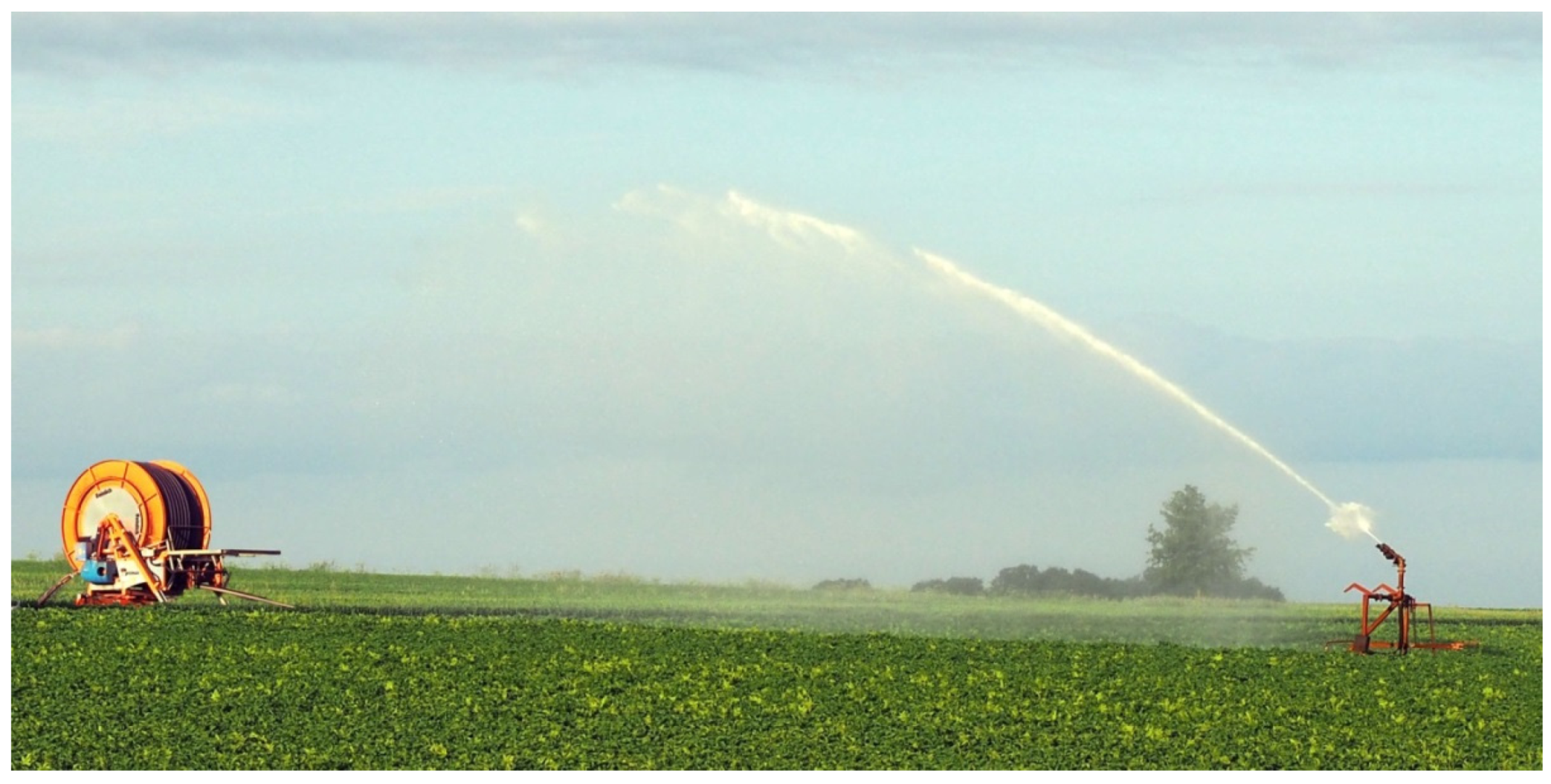
Sprinkler irrigation introduced in the 1950s is still considered by farmers to be the most suitable and economical method for growing crops under regional conditions [6]. It is typically performed by turntable machines with rain-gun trolleys. The trolley is pulled along the irrigation track by its PE (polyethylene) hose, which is wound up by the drum. Slow rotation is provided by a turbine driven by the irrigation water. Field strips of several hundred meters in length and about 30 m width can be irrigated in one application with a typical depth of 30 mm. Figure 2 shows a unit in operation.

Figure 2. Sprinkler irrigation with pipe drum and rain-gun trolley.

Figure 2. Sprinkler irrigation with pipe drum and rain-gun trolley.

Water is taken from the Quaternary aquifer at a depth of about 100 m by pumping stations owned and operated by the farmers. All wells, groundwater withdrawals, and irrigated areas need permission from the local environmental and water authorities [7]. Applications must be backed by hydro-geological expertise. The irrigation water depth for the respective areas is limited to 70 mm per summer over a seven-year average, i.e., higher abstractions in dry years can be compensated by lower ones in wetter summers. Nearly 700 km² (50%) of the county is farmland. Since the 1950s, when irrigation was introduced, irrigated areas were enlarged to about 550 km². The irrigation depth of 70 mm would then need a volume of 38.5 hm³ per year. Depending on the summer weather, the actual volumes varied in the observed years between less than 10 and about 50 hm³. For the catchment area of 1434 km² the maximum abstraction corresponds to a 35 mm depth, which is about 5% of mean annual basin precipitation (1955–2012) or more than a quarter of the precipitation in a very dry summer (May–October 1959: 131 mm). Effects on low flows and groundwater storage must be expected. Figure 3 shows the development of registered areas and of the groundwater abstractions for irrigation 1977–2012.

Figure 3. Development of irrigation areas and groundwater abstraction in the catchment; registration of areas and groundwater abstractions began in 1977, data: County of Uelzen.

Figure 3. Development of irrigation areas and groundwater abstraction in the catchment; registration of areas and groundwater abstractions began in 1977, data: County of Uelzen.

With the objective of ensuring a sustainable management of water resources, the water and environmental authorities observe this development. The chamber of agriculture initiated an interdisciplinary study of irrigation possibilities for different climate change scenarios and adapted technologies [8].

4. Low Flows, Climate, and Groundwater Abstractions

At the Bienenbüttel gauging station, daily flows have been recorded since 1956. In assessing low flows and water levels, the absolute minima of each year are of little significance. Since the damage potential of low flow events also depends on their duration, the lowest arithmetic mean LQ_xd of x consecutive daily flow values of every year is used as the assessment variable. The annual values LQ_xd are determined for durations of typically x = 3, 7, 20 days for each water budget year. In northern Germany, the relevant low flow events are to be expected in the summer months (May–October).

The time series 1956–2012 of annual low flows LQ₂₀ at the Bienenbuettel/Ilmenau gauging station in Figure 4 reveals a significant (t-test) linear downward trend. The strong fluctuations can be interpreted as a sequence of different negative and positive trends. It seems that after a decline until the end of the 1970s, there is no further clear trend, but instead there is a high variability in annual low flows. The physical causes of these variations and inconsistencies of the low flow hydrograph can be due to both weather processes and anthropogenic influences. Mean annual basin precipitation is also depicted in Figure 4, derived by the Thiessen polygon method using the data of 13 stations in and around the catchment. It increased statistically by about 100 mm during the observation period while evapotranspiration was stimulated by the warming of mean summer temperatures of about 1 K. In Germany, the hydrological year is divided into the winter half-year (November to April) and the summer half-year (May to October). The latter represents roughly the vegetation season. Mean values of catchment precipitation and air temperatures in the two seasons in Lueneburg are given in Table 2. Essential impacts are to be expected from groundwater abstractions for irrigation, which are recorded by water meters at all irrigation wells. Annual total values for the catchment expressed in m³/s are also shown in Figure 4.

Figure 4. Annual basin precipitation P, summer temperature Ts, 20-day low flows LQ_20, and groundwater abstractions QI, Ilmenau Basin at Bienenbüttel, 1977–2012.

Figure 4. Annual basin precipitation P, summer temperature Ts, 20-day low flows LQ_20, and groundwater abstractions QI, Ilmenau Basin at Bienenbüttel, 1977–2012.

5. Multiple Regression Analysis—Low Flows

Multiple regression is a classic method of data analysis [9] but is rarely used in contemporary hydrology. Even state-of-the-art studies on low flows [2] mostly use regression only in its simple version and for trend analysis. Unlike the simple trend analysis of low flows which relates all changes to time, multiple regression enables the assessment of statistical associations among the response variable and primarily independent multiple covariates. The relationship established in Equation (1) assumes annual low flows:

$$LQ{x}_t=L{Q}_0+a\cdot P{W}_t+b\cdot P{S}_t+c\cdot PJ_{t-1}+d\cdot T{W}_t+e\cdot T{S}_t+f\cdot Q{I}_t$$

(1)

where,

• LQx_t:→ x days low flow in the year t in m³/s;
• LQ₀:→ base value of low flow in m³/s;
• PW_t:→ winter precipitation in the year t in mm;
• PS_t:→ summer precipitation in the year t in mm;
• PJ_t-1:→ precipitation of preceding water year in mm;
• TW_t:→ mean air temperature, winter of year t in °C;
• TS_t:→ mean air temperature, summer of year t in °C;
• QI_t:→ groundwater abstraction for irrigation in year t in mm.

With the data set of 1977–2012, there is an over-determined system of 36 equations. Reducing the system by the Gauss-Jordan algorithm determines the seven unknowns, i.e., the base value and the six coefficients a to f, according to the least squares criterion. For the 20-day period, low flows are obtained:

$$LQ{M}_{\mathrm{20t}}=4.48+0.0030P{W}_t+0.00094P{S}_t+0.0033PJ_{t-1}+0.022T{W}_t-0.049T{S}_t-0.102QI$$

(1a)

The coefficients, factors, or weights represent the sensitivity of low flow values to unit changes of the variables. Table 1 shows the correlation coefficients of the variables to one another and to the dependent variable low flow. Correlations with |R| > 0.33 are significant at the 95% level. In addition, the coefficients concerning the registered irrigation areas AI are listed. These values are expected to have an influence on the assessment of applied water volumes in Section 7.

Table 1. Partial correlation coefficients of variables, time series 1977–2012.

variable	PW	PS	PJt-1	TW	TS	QI	AI
PW	1
PS	0.127	1
Pt-1	0.194	−0.092	1
TW	0.490	0.168	−0.020	1
TS	0.186	−0.194	0.181	0.336	1
QI	0.033	− 0.618	0.320	0.199	0.472	1
Ai	0.096	0.259	0.312	0.222	0.310	0.324	1
LQ20	0.265	0.578	0.116	−0.059	−0.317	− 0.735	−0.220

Table 1. Partial correlation coefficients of variables, time series 1977–2012.

variable	PW	PS	PJt-1	TW	TS	QI	AI
PW	1
PS	0.127	1
Pt-1	0.194	−0.092	1
TW	0.490	0.168	−0.020	1
TS	0.186	−0.194	0.181	0.336	1
QI	0.033	− 0.618	0.320	0.199	0.472	1
Ai	0.096	0.259	0.312	0.222	0.310	0.324	1
LQ20	0.265	0.578	0.116	−0.059	−0.317	− 0.735	−0.220

The overall correlation coefficient between the n = 36 calculated values and the data is R = 0.865 (R² = 0.75). As expected, it is considerably higher than all partial coefficients and thus demonstrates the advantage of multiple regression over simple regression analysis. The coefficient of variation, i.e., the average deviation between data and values by Equation (1a), is 9%.

The groundwater abstraction for irrigation QI has a significant negative correlation with summer precipitation PS and a positive one with summer temperature TS, an indication for disciplined and frugal water allocation by the farmers. Higher rainfall reduces the need for irrigation, while higher temperatures increase evaporation and irrigation requirements.

As indicated by the correlation coefficients, the information of the values PS and TS with relevance for low flows seems to be largely included in the time series QI. The influence of winter temperature TW on low flows is negligible (see Equation (1a)). Therefore, a further multiple regression for LQ₂₀ with variables as in Equations (1) and (1a), but without PS, TW, and TS was performed:

$$L{Q}_{\mathrm{20t}}=4.22+0.0032P{W}_t+0.0033PJ_{t-1}-0.1092QI$$

(1b)

The correlation coefficient between the observed and calculated low flows is R = 0.863 and the coefficient of variation is CV = 9.2%. Thus, the result is practically the same as for Equation (1a) and the assumption is confirmed.

Table 2 contains the mean values from 1977 to 2012 of the input variables in the first line. By multiplying with their coefficients or weights according to Equations (1a) and (1b), respectively, their contribution to the total value of the low flow is obtained (following lines).

First of all, the coefficients are statistical weights that do not necessarily represent partial physical flows. However, since the coefficients of the three parameters used in both Equations (1a) and (1b) have similar to equal values, it is concluded that the computed partial flows are not purely mathematical regressive values but do stand for real water flows. It is worth noting the high contributions of winter and the previous year’s precipitation to low flows because of their importance for groundwater recharge.

Table 2. Coefficients and partial flows of LQ₂₀ according to Equations (1a) and (1b).

variable	LQ0 m3/s	PW mm	PS mm	Pj-1 mm	TW °C	TS °C	QI mm	Σ LQcalc m3/s
mean values		336	376	708	3.79	14.7	18.1
coefficients 1a		0.0030	0.00094	0.0033	0.022	−0.0494	−0.1023
flow	4.48	1.01	0.35	2.34	0.08	−0.73	−1.85	5.68
coefficients 1b		0.0032	-	0.0033	-	-	−0.1092
flow	4.22	1.08	-	2.34	-	-	−1.98	5.68

Table 2. Coefficients and partial flows of LQ₂₀ according to Equations (1a) and (1b).

variable	LQ0 m3/s	PW mm	PS mm	Pj-1 mm	TW °C	TS °C	QI mm	Σ LQcalc m3/s
mean values		336	376	708	3.79	14.7	18.1
coefficients 1a		0.0030	0.00094	0.0033	0.022	−0.0494	−0.1023
flow	4.48	1.01	0.35	2.34	0.08	−0.73	−1.85	5.68
coefficients 1b		0.0032	-	0.0033	-	-	−0.1092
flow	4.22	1.08	-	2.34	-	-	−1.98	5.68

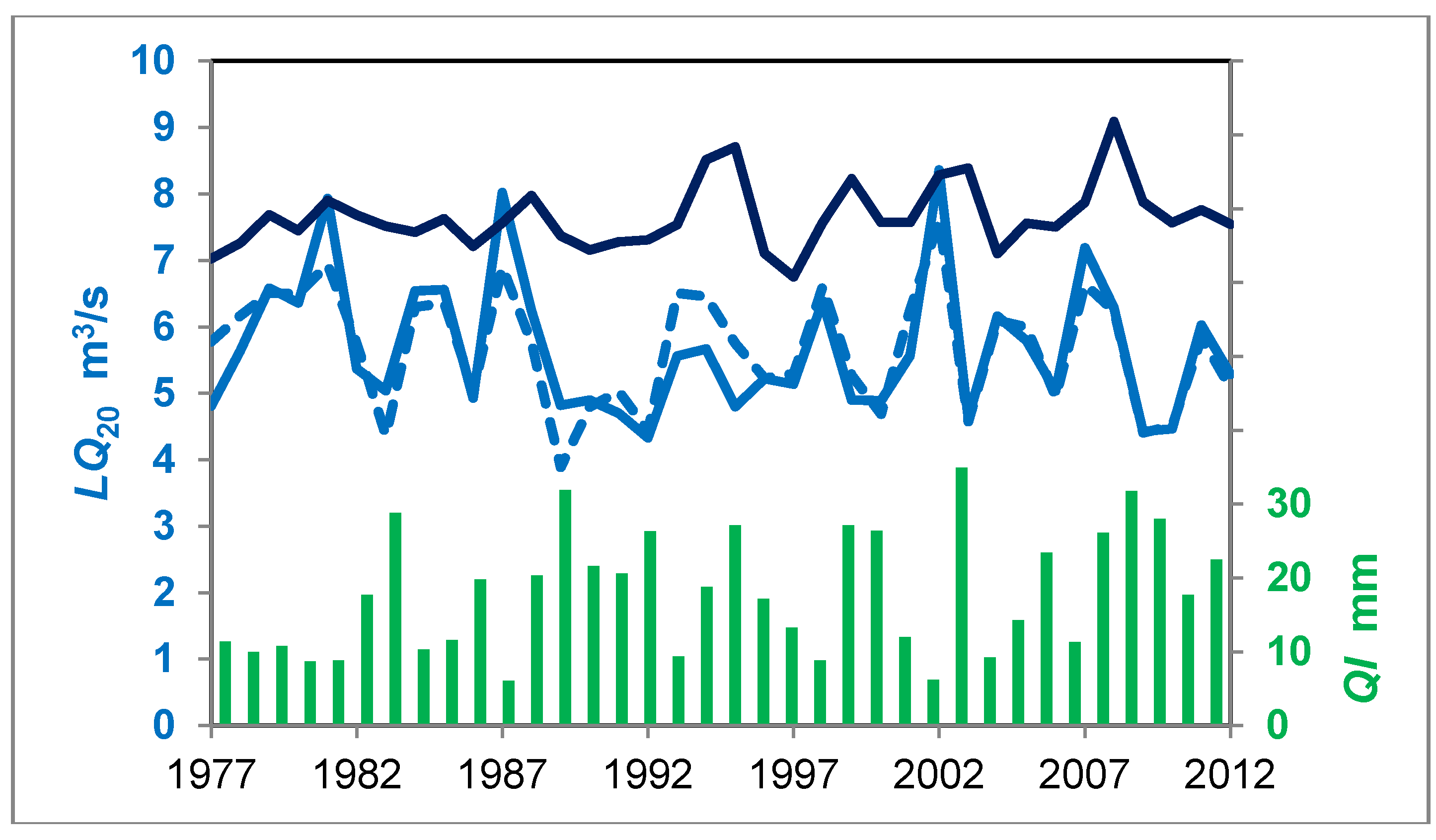
In this study, one focus is on the influence of groundwater abstraction. As shown in Table 2, the respective average annual reduction of low flow LQ₂₀ is about 1.9 m³/s or 25%. Observed low flows from 1977 to 2012 and values computed by Equation (1b) are depicted in Figure 5. Annual amounts of groundwater abstraction are shown for comparison. By omitting the last term of Equation (1b), the influence of groundwater abstraction QI is eliminated and a time series of hypothetical uninfluenced low flows obtained. The resulting hydrograph is also shown in Figure 5.

Figure 5. Observed and computed (Equation (1b), dashed line) annual low flow values, computed low flows uninfluenced by abstractions (above, dark blue), and groundwater abstractions QI.

Figure 5. Observed and computed (Equation (1b), dashed line) annual low flow values, computed low flows uninfluenced by abstractions (above, dark blue), and groundwater abstractions QI.

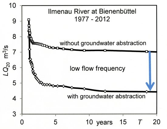
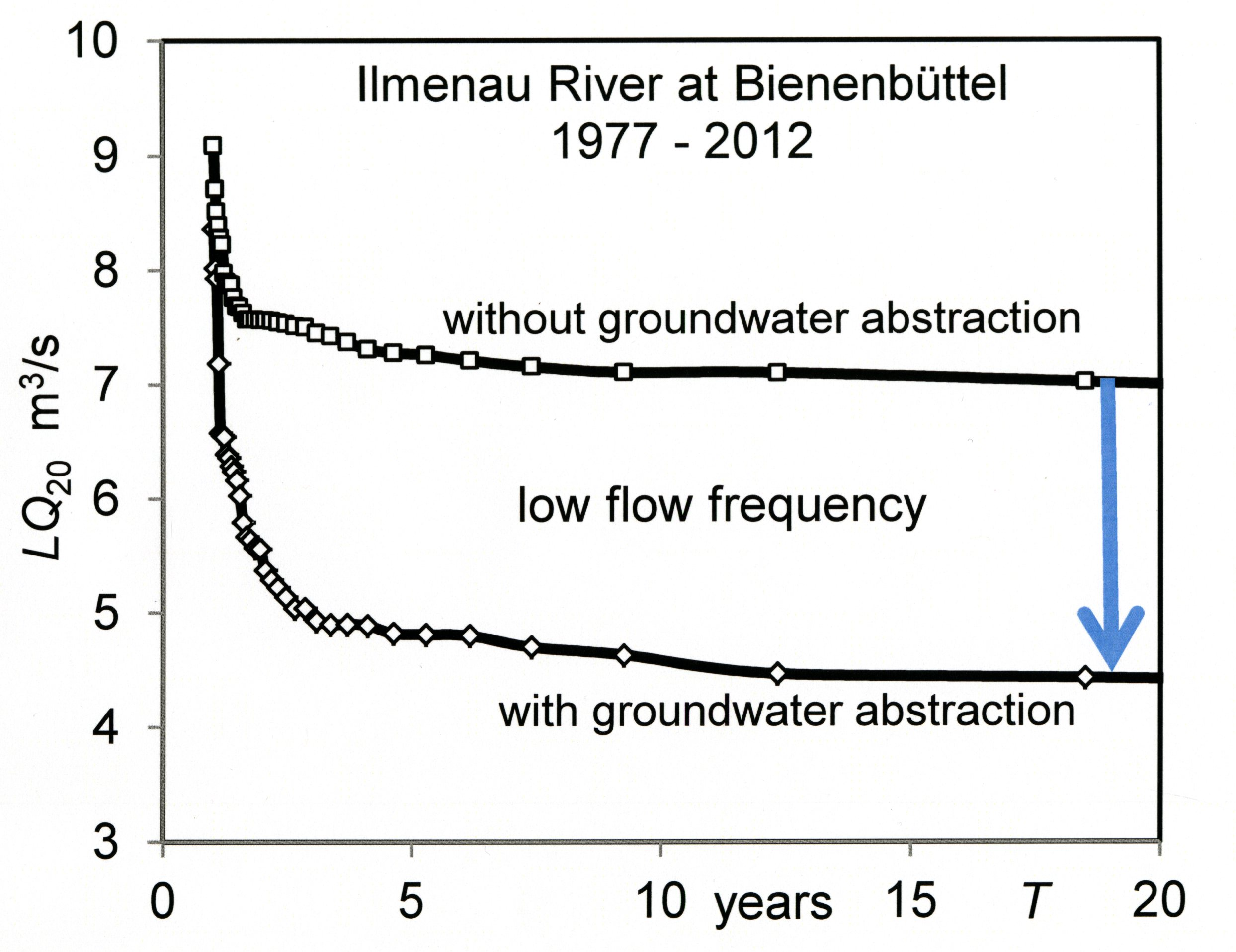
As reflected by the above equations, the reduction of annual low flows is higher in drier years with more groundwater withdrawal than in moderate years. This is also shown by the empirical probability curves in Figure 6. These curves were determined according to the method of “plotting positions”. Data and the computed uninfluenced low flows are respectively sorted in decreasing order, and statistical return intervals T are determined for every value according to Equation (2):

$$T=(n+1)/(n+1-m)$$

(2)

with

• T:→ return interval in years;
• n:→ number of data, length of data set;
• m:→ ranking from 1 (greatest value) to n (lowest value).

Figure 6. Frequency analysis of 20-day low flows.

Figure 6. Frequency analysis of 20-day low flows.

The difference between probable low flows with and without groundwater abstraction increases with the recurrence interval T. The regressions and calculations described above were also carried out for time series of low flows of three- and seven-day durations. Comparable results and relationships following the same pattern have been obtained.

6. Groundwater Impacts

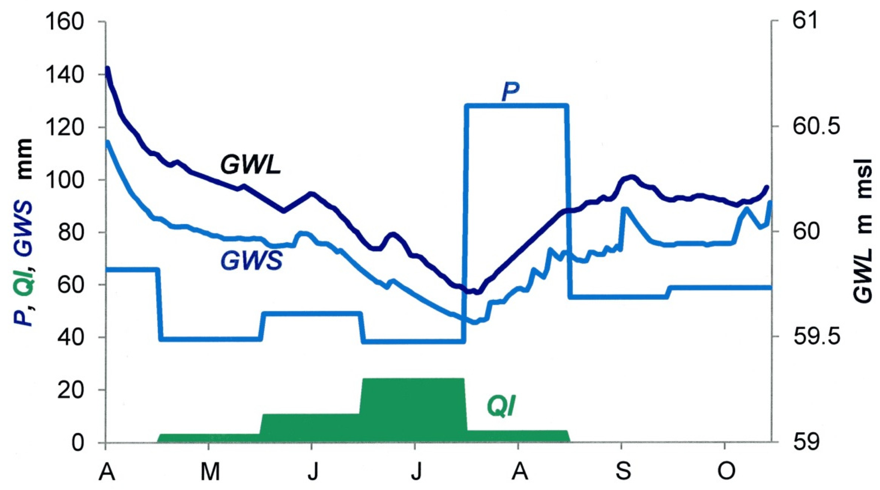
Low flow occurs when direct runoff has ceased and the river only carries baseflow, i.e., groundwater outflow from the adjacent aquifer. Therefore, the lowest annual low flow coincides with the lowest groundwater level. Groundwater withdrawal lowers the level but also reduces the outflow, preserving, in a sense, the aquifer. At the end of the irrigation period, with lower evapotranspiration in the autumn, rainfall leads to a recharge and recovery of the aquifer. The respective hydrographs of monthly precipitation P and abstraction QI and daily groundwater levels GWL for a sub-catchment of the Ilmenau Basin in the summer season of 1994 are shown in Figure 7. Daily values of mobile groundwater storage GWS obtained in another study [10] are also depicted. These values were computed from baseflow separated from total flow by using a nonlinear reservoir algorithm.

In the same study, it was found that, under regional conditions, only about 70% of irrigation water is lost for the groundwater, since 30% infiltrates back or prepares the soil for infiltration of the next rainfalls. These findings match the results obtained in a different approach [11].

While low flows are lowered by groundwater abstractions, the long-term volumes and water levels of the aquifer are little affected. Depressions are only observed at some places at higher parts of the watershed. Water quantity does not pose substantial problems. However, the preservation of long-term groundwater quality by a careful use of fertilizers and agrochemicals remains an important issue [12].

Figure 7. Monthly rainfall P, groundwater abstraction QI, daily values of groundwater level GWL, and computed mobile groundwater storage GWS, Eisenbach catchment, summer 1994.

Figure 7. Monthly rainfall P, groundwater abstraction QI, daily values of groundwater level GWL, and computed mobile groundwater storage GWS, Eisenbach catchment, summer 1994.

7. Multiple Regression—Groundwater Abstraction

Except for some smaller test areas, groundwater abstraction data are available per irrigation season (April–October) of every year, while precipitation and temperature data are available monthly and per season. As given in Table 1, groundwater abstraction QI is significantly correlated with summer rainfall PS, summer temperature TS, and irrigated areas AI. The corresponding regression had the following result:

$$Q{I}_t=-11.6-0.0743P{S}_t+2.56T{S}_t+0.000434A{I}_{t}R=0.82$$

(3a)

While the correlation coefficient is high, the coefficient of variation, i.e., the mean deviation of calculated values from abstraction data, is 26% and thus not quite satisfying. This is mainly due to a fuzziness of the term summer rainfall (April–October). For irrigation requirements and management, it makes a big difference whether rains fall early in the growing period rather than during or even after harvest. A first step to improving the relationship was the substitution of the values of total summer precipitation (April–October) with those of the main irrigation period (May–August). A correlation coefficient of R = 0.86 and a mean deviation of 23% were obtained.

However, rainfall depth has more or less importance depending on the month of the irrigation period. Monthly data of groundwater uptake in some smaller test areas in the watershed [13] from 1990 to 2011 showed the following temporal distribution of volumes: April 3%, May 17%, June 30%, July 29%, August 15%, September 4%, and October 2%. Monthly rainfalls were multiplied by the percentages. The sum of these products for every year represents a weighted mean value for replacing the total summer rainfall. Indeed, the partial correlation of groundwater abstraction with the new variable is closer (R = −0.73) than with summer rainfall (R = −0.62; Table 1). The improved relationship is:

$$Q{I}_t=-9.02-0.419Pwe{i}_t+2.48T{S}_t+0.0004A{I}_{t}R=0.89$$

(3b)

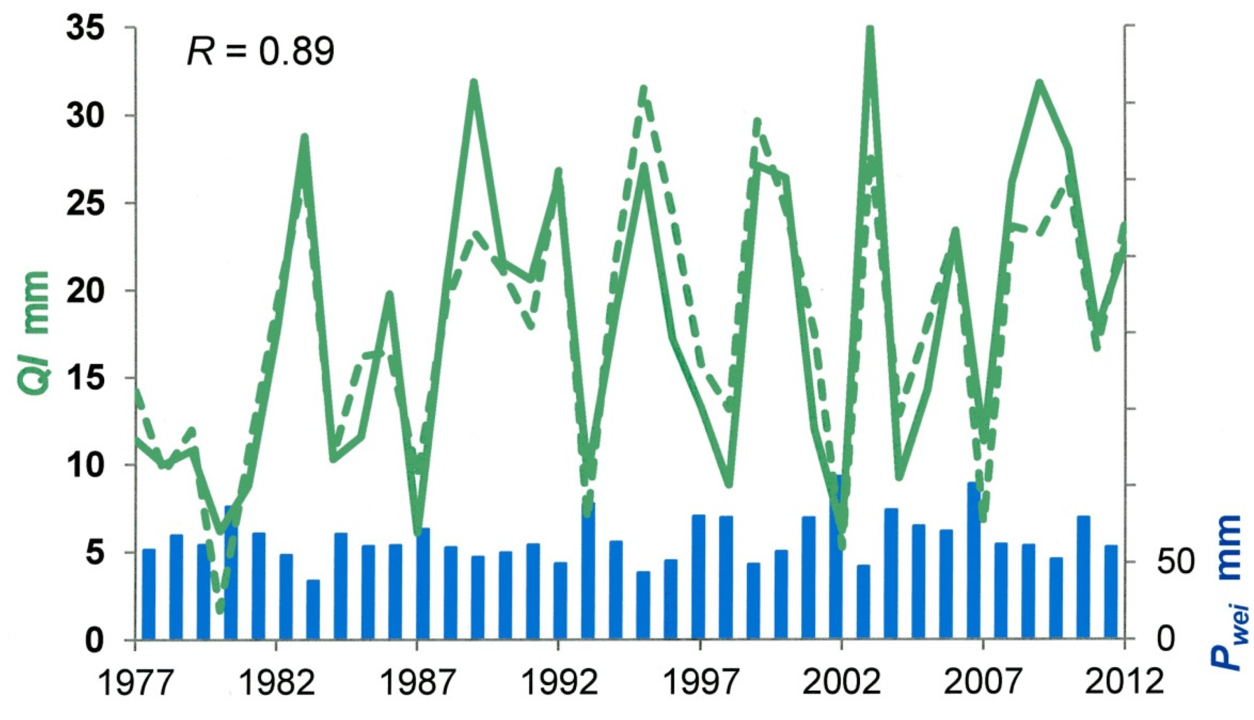
The result is shown in Figure 8. The annual weighted means of seasonal rainfall P_wei are plotted for comparison. The mean deviation between data and computed values is 21%. This seems high, but it must be seen in the context that the variation coefficient (standard deviation/mean) of the annual abstractions is more than double (47%). It is also noticeable that this variation is essentially preserved in the computed series of QI (42%), though they are based on variables with much lower variation coefficients, P_wei (23%), TS (4%), and AI (19%). Other than with single regression, where variation is determined (and damped) by the independent variable, this is possible by the superposition effects of multiple regression.

Figure 8. Recorded and computed (Equation (3b), dashed line) annual groundwater abstractions QI, weighted means of seasonal rainfall P_wei.

Figure 8. Recorded and computed (Equation (3b), dashed line) annual groundwater abstractions QI, weighted means of seasonal rainfall P_wei.

8. Conclusions

Multiple regression analysis allows distinguishing and quantifying the influence of different climatic and man-made variables such as precipitation, temperature, and groundwater withdrawal on annual low flows. It was found that groundwater abstraction for irrigation in the Ilmenau Basin accounts for an average decrease of low flows of about 25%. The groundwater levels and long-term volumes recover during the winter season. The annual abstraction volume is highly correlated with rainfall depth in the vegetation season, summer air temperature, and irrigation area. It is thus evident that groundwater abstractions in the Ilmenau Basin are based closely on actual irrigation requirements.