7.1. A Portfolio Decision Analysis Model for Mitigation Project Selection
This analysis is set in the context of a finite sum of money available to allocate to a range of potential natural disaster mitigation projects. The decision is to choose the best subset of projects within a given budget, where the term “best” refers to the combination of projects offering the greatest cost-effectiveness. This in turn is based on the projects’ values (as determined by the multi-criteria framework), and their capital and operational costs. This is a portfolio selection problem.
A simple heuristic for selecting a portfolio of projects may be the following:
- Step 0
Let the overall mitigation project budget be $B.
- Step 1
Of the available projects, select the one with the highest cost-effectiveness ratio (cost effectiveness ratio = CER = , where the project value is the score determined from the multicriteria model, scaled onto [0, 1]; this ratio allows a comparison of projects; those that offer greater value per dollar spent are preferred) (CER).
- Step 2
Check that the cost of this project is lower than $B.
If yes, call this project P[i] (where i = 1, 2, … is the selection rank of the project in the portfolio) and include it in the portfolio. Adjust the available budget to $B = $B-c[i] where c[i] is the cost of project P[i]. Go to Step 1.
If no, select the project with the next highest cost effectiveness ratio (CER). Go to Step 2.
When no further projects can be selected, stop.
The portfolio of mitigation projects is the set {P[1], P[2], P[3], ….}.
This heuristic may be appropriate when:
There are a limited number of alternative projects
The projects are independent of each other
There are no constraints on the selection process.
The last two points require some explanation. Projects can be considered independent of one another if the impact (or value) of each of the projects is the same whether or not the other project was undertaken. For example, two mitigation measures might be proposed to address a single hazard in some community, e.g., building a levee, and physically moving home and infrastructure to higher ground, say, to address local flooding in a town. If the levee is built, the likelihood of flooding is minimised, and so, the value of moving the community is reduced. Similarly, if the community is moved, the threat to people and homes is minimised, and so, the value of the levee is reduced. Thus, these two mitigation measures are not independent. At the local level, where the decision is most likely to be around alternative measures to address the threat posed by a single hazard, the possibility of the dependence of the alternative options will likely exist. However, the decision at this level is likely to be around the single best option to address the threat. On the other hand, at the national level (where funding decisions are most likely made), the decision maker(s) are likely to be faced with choices amongst a range of potential mitigation projects across multiple hazards, a range of scales and in multiple jurisdictions/communities. These projects are then unlikely to exhibit the kind of interactions illustrated in the example above, and projects can then be considered independent.
The decision framework calls for the selection of the subset of potential mitigation projects that were most cost-effective in reducing risks to the community and maximizing social benefits. This framework evaluates each member of a set of potential mitigation options under a number of criteria; what remains is to identify the subset of projects that contains the most cost-effective projects, given the overall budget available for mitigation projects.
Furthermore, the selection of a portfolio of natural disaster mitigation projects is likely to be constrained in several ways:
- (1)
Budget considerations will make it unlikely that every potential project will be able to be funded.
- (2)
A selection panel is likely to impose an upper bound on the funds available for any single project.
- (3)
The selection panel is likely to want to fund multiple projects. This will have several advantages:
- (i)
Multiple projects means diversification of project impacts, both geographical and across domains
- (ii)
Diversification will necessarily reduce the overall portfolio risk.
Other constraints may also be placed on the selection of projects by a decision making group.
Determining the best subset of alternative projects to select is a portfolio decision analysis (PDA) problem [
33]. PDA has its roots in the field of quantitative finance, through Harry Markowitz’s approach to modern portfolio theory [
34], which focuses on assessing both the risk and the returns of an asset portfolio. This approach is now widely used in R&D project selection.
The optimal selection of projects to be included in the portfolio can be achieved using linear programming, which is designed to achieve the best outcome for some objective (for example, the maximum profit or the lowest cost), given constraints on how the allocation may be achieved. It is a modelling requirement that the objective and constraints can all be represented by linear relationships.
Assume that n mitigation projects are under consideration for selection to a portfolio. A typical set of constraints for project selection might comprise
a total funding budget of B dollars is available
the cost of project i is ci dollars
the value score of project i is vi units on [0, 1]
at least s projects must be selected (for diversification)
at most t projects must be selected
at most r dollars can be spent on any one project.
In practice, further constraints can be added to this or any of these constraints removed.
Define a variable Yi to be a binary variable, describing whether or not a project i is selected into the portfolio or not. Thus, Yi is one if the project is selected, and Yi is zero if the project is not selected.
Objective function:
(While costs are additive, the project values are, by their definition, not additive. By this, it is meant that a portfolio of multiple projects may result in an aggregate value of greater than one, even though individual m project value is defined to have an upper bound of one. Thus, the aggregated value of the portfolio cannot be interpreted in the same way as an individual project’s value. In any event, a greater aggregated portfolio value is better than a lesser one.) Maximise v1Y1 + v2Y2 + v3Y3 + … + vnYn;
Subject to:
Linear problem constraints:| c1Y1 + c2Y2 + c3Y3 + … + cnYn ≤ B | (total cost of all projects in the portfolio less than $B) |
| ci Yi ≤ r for all projects i = 1, 2, … , n | (at most r dollars can be spent on any one project) |
| Y1 + Y2 + Y3 + … + Yn ≥ s | (at least s projects selected, for diversification) |
| Y1 + Y2 + Y3 + … + Yn ≤ t | (at most t projects selected) |
Non-negativity constraints:
| Yi = 0 or 1 | for all projects i = 1, 2, …, n |
Powerful software tools exist to rapidly produce a solution to a linear optimisation model, such as the one presented above. For models of relatively small dimension, the Solver add-in for an Excel spreadsheet may be appropriate.
7.2. An Illustrative Example: Choosing a Portfolio of Mitigation Projects
Table 9 displays information for a set of nine potential mitigation projects. Assume that a budget of $45 million is available to allocate to projects in this funding round.
The project cost (Column 2) is essentially the present value of all costs related to the project (in $ million). The total cost of all projects together is $133 million, implying that not all projects can be funded given the budget. The multi-criteria “benefit score” (Column 3) is the overall value score associated with each project using a framework such as that developed in this paper. The cost-effectiveness ratio (Column 4) is the value score divided by the cost.
Project 4 clearly offers the greatest benefit (as defined by the multicriteria framework), but also has the greatest cost. By contrast, Project 5 has the lowest cost of all, but offers a relatively low benefit.
Applying the simple heuristic model would yield the following steps:
Choose the most cost-effective project. This is Project 5 (CER is largest: 20.00). The cost of this project is $2 million, leaving $43 million available for other projects.
Of the remaining projects, Project 2 has the largest cost effectiveness ratio (CER: 12.25). As the cost of this project is $4 million, it is added to the portfolio. The available budget is now $39 million.
Projects 9 (CER = 6.40, cost = $10 million), 6 (CER = 5.67, cost = $6 million), 8 (CER = 4.43, cost = $7 million) and 3 (CER = 3.00, cost = $15 million) are then added iteratively, reducing the available budget to $29 million, $23 million, $16 million and $1 million at successive iterations. No further project can be added to the portfolio due to the budget constraint.
The final portfolio thus consists of Projects 2, 3, 5, 6, 8 and 9, with $1 million remaining.
Assume now that the selection of the portfolio of mitigation projects is constrained in the following ways (further constraints may also be placed on the selection of projects):
A total funding budget of $45 million dollars is available.
At least three projects must be selected (to ensure diversification).
At most $30 million dollars can be spent on any one project.
The optimal selection of projects to be included in the portfolio using the Excel spreadsheet Solver routine is identical to that produced by the simple heuristic: Projects 2, 3, 5, 6, 8 and 9, costing $44 million.
Table 10 displays the spreadsheet workings and optimised result for the linear programming model.
Further analysis may reveal changes to this optimal solution if constraints are altered. For example,
Table 11 displays the make-up of the optimal portfolio as the available budget changes from $20 million through to $100 million.
Table 11 shows that as the budget increases, more projects can be undertaken. However, the combination of projects changes:
Projects 6 and 8 are selected in every portfolio
Projects 5 and 9 are included in five of the six portfolios: Project 5 is included when the budget is lower, and Project 9 is included when the budget is higher
Project 2 is included in four portfolios, mostly when the budget is low
Projects 1, 3 and 7 are only included in half of the portfolios and only when the budget is high
Project 4 is never included in any portfolio, as it is by far the costliest project and, thus, offers the lowest value for the money.
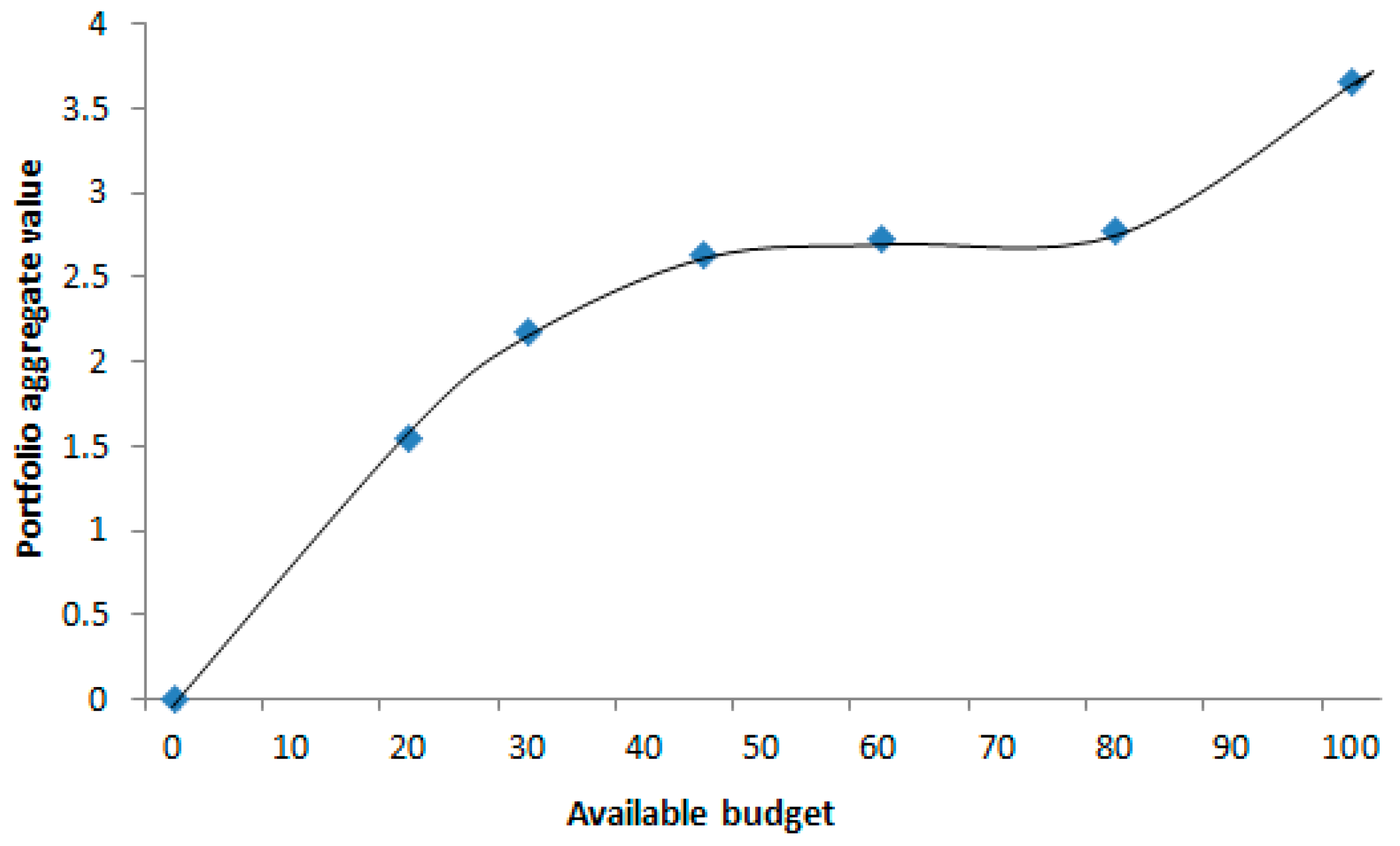
Figure 9 shows the increase in the aggregate value of the portfolio as the available budget increases. The slope of the curve is steepest for low budget amounts (less than $30 million, say) and for high budget amounts (greater than $80 million, say). These are the ranges in which an extra $1 million leads to the greatest increase in aggregate value. A careful study of
Figure 9 should focus high level policy makers on the most cost effective budget for the mitigation decision.


