1. Introduction
Smart farming represents the use of information and communication technology systems applied in agriculture with the objective of obtaining better results, greater performance and higher quality production with safety and precision while optimizing human work [
1,
2].
From these new technologies, a cultivation area can be divided into as many plots as it has internal differences supported by soil analysis and each plot can receive a customized treatment to obtain the maximum benefit from it. This is also known as precision agriculture [
3,
4,
5].
However, it is necessary to characterize the variability of the chemical and physical attributes of the soil through a representative sample of such variations. So, soil analysis is the only method that allows, before planting, to recommend adequate amounts of correctives and fertilizers to increase crop productivity and, as a consequence, crop production and profitability. Soil science is considered a strategic research topic for precision agriculture and smart farms [
6,
7].
The clay content defines the texture of the soil. It interferes with several factors including plant growth and productivity, water infiltration into the soil and its storage, retention and transport, availability and absorption of plant nutrients, living organisms, soil quality, productivity and temperature, levels of structure and compaction, soil preparation, irrigation and fertilizer efficiency. Therefore, the clay content plays a fundamental role in crop productivity [
8].
The traditional way of collecting soil in the fields and analyzing it in the laboratory is the most accurate, but it takes time and uses an alkaline solution that needs to be neutralized before wasting [
9]. New research has been proposed to optimize this, but with limitations. Satellite images are important for obtaining quick information on the surface of soils in large areas. However, mapping large areas of soil presents difficulties as most areas are usually covered by vegetation [
10].
The use of spectral images expands the capacity of studies in several areas and their application has been growing in agriculture in order to recognize patterns [
11,
12,
13]. For these types of analyses, two well-known scientific methodologies are used: Spectroscopy and imaging. Optical spectroscopy is a term used to describe the phenomena involving a spectrum of light intensities at different wavelengths. Imaging can be conceptualized as the science of image acquisition of the spatial shape of objects. Currently, the most advanced way to capture images is digitally [
14].
Multispectral and hyperspectral imaging systems are image analysis techniques that are also based on capturing the same image at different wavelengths.The difference consists in the number of captured wavelengths: While multispectral systems use up to 10, hyperspectral systems can exceed 100 wavelengths, with the latter generating larger amounts of data [
15].
Since single-board computers have become more accessible to the general public, the Raspberry Pi has become one of the more popular systems, mainly in the scientific community, promoting research in IoT and all features involved [
16,
17]. Leithardt et al. [
18] and Felipe Viel et al. [
19] developed works that exemplified the application of the Raspberry Pi in IoT.
In addition, machine learning tools as Partial Least Regression (PLSR) have been applied for multivariate calibration in soil spectroscopy [
20], images [
21] and sensor data [
22]. These algorithms eliminate variables that do not correlate with the property of interest, such as those that add noise, non-linearities or irrelevant information [
23].
Considering the importance of research in areas involving soils (agriculture, geochemistry, geology), the ability to use devices such as the Raspberry Pi and the use of computer vision techniques such as spectral imaging, the following research problem was defined: “Is it possible to use multispectral imaging techniques to predict clays?”.
The main objective is to develop a computer vision system to predict the amount of clay in the soil using multispectral imaging techniques on a Raspberry Pi device. The relevance of this work is in the absence of a fast, mobile, cheap and non-destructive method to measure clay content in soil.
This article is structured in six sections.
Section 2 presents an approach to the soil texture and colors, multispectral images, machine learning and OpenCV libraries.
Section 3 describes the related works, while
Section 4 presents materials and methods employed.
Section 5 shows the results of the implementation and its discussions. Finally
Section 6 is intended for conclusions and future works.
3. Related Work
There are several works in the field of multispectral imaging in the most diverse areas of application. The selected articles’ subjects are related to multispectral data, smart farm and soil prediction.
In 2014, Svensgaard et al. built a mobile and closed multispectral imaging system to estimate crop physiology in field experiments. This system shuts out wind and sunlight to ensure the highest possible precision and accuracy. Multispectral images were acquired in an experiment with four different wheat varieties and two different nitrogen levels, replicated on two different soil types at different dates. The results showed potentials, especially at the early growth stages [
38].
In 2015, Hassan-Esfahan developed an Artificial Neural Network (ANN) model to quantify the effectiveness of using satellite spectral images to estimate surface soil moisture. The model produces acceptable estimations of moisture results by combining field measurements with inexpensive and readily available remotely sensed inputs [
39].
Treboux and Genoud presented in 2018 the usage of decision tree methodology on segregation of vineyard and agricultural objects using hyperspectral images from a drone. This technique demonstrates that results can be improved to obtain 94.27% of accuracy and opens new perspectives for the future of high precision agriculture [
40].
Žížala et al. performed in 2019 an evaluation of the prediction ability of models assessing soil organic carbon (SOC) using real multispectral remote sensing data from different platforms in South Moravia (Czechia). The adopted methods included field sampling and predictive modeling using satellite data. Random forest, support vector machine, and the cubist regression technique were applied in the predictive modeling. The obtained results show similar prediction accuracy for all spaceborne sensors, but some limitations occurred in multispectral data [
41].
Lopez-Ruiz et al. presented in 2017 the development of a low-cost system for general purposes that was tested by classifying fruits (putrefied and overripe), plastic materials and determining water characteristics. This work shows the development of a general-purpose portable system for object identification using Raspberry Pi and multispectral imaging, which served as the basis for the present study [
42].
Table 1 compares articles regarding the application, data analysis, type of sensors and properties, including the proposed work. The following criteria allowed comparison of the proposed model and the aforementioned studies identifying relevant characteristics for evaluation:
- 1.
Sensors: This shows the sensors used in the related studies;
- 2.
Analysis: This identifies which tool is used for data analysis. In other words, it identifies how results were generated for decision making or information to users;
- 3.
Spectral range: This informs the type of spectral image employed (multispectral or hyperspectral);
- 4.
Application: This describes the object, material or scenery analysed.
No study directly related to clay prediction in precision agriculture was found in the literature based on multispectal analysis using LED lamps. The research that presented the multispectral data for decision making mostly made use of resources from satellite images or non-portable solutions, differently to as suggested in the present article.
4. Materials and Methods
A total of 50 soil samples were selected from different collection points of the Vale do Rio Pardo/RS, Brazil, where the clay concentrations ranged from 4% to 72%. These samples were supplied by the Central Analitica soil laboratory (Santa Cruz do Sul, Brazil), where they were dried in a MA037 oven (Marconi, Piracicaba, Brazil) with air circulation for a period of at least 24 h at a temperature between 45 and 60 ºC. Afterwards, the samples were ground in a NI040 hammer mill (Marconi, Piracicaba, Brazil), with 2 mm strainer, and stored in cardboard boxes.
This work proposes a system that predicts the amount of clay contained in soil samples using a panel of LED lamps of various colors. The lamps were arranged around a Raspberry Pi NoIR microcamera with OV5647 sensor (OmniVision Technologies). The OV5647 is a low voltage, high performance, 5 megapixel CMOS image sensor that provides up to 2592 × 1944 video output and multiple resolution raw images via the control of the serial camera control bus or MIPI interface. The sensor has an image array capable of operating up to 15 fps in high resolution with user control of image quality. The camera is connected to the BCM2835/BCM2836 processor on the Pi via the CSI bus, a higher bandwidth link that carries pixel data from the camera back to the processor. This bus travels along the ribbon cable that attaches the camera board to the Pi. So, the OV5647 sensor core generates streaming pixel data at a constant frame rate [
43].
The microcamera (Pi NoIR v1.3) was coupled to a Raspberry Pi 3 Model B computer that processes the captured images. This device was launched in February 2016 and it uses a 1.2 GHz 64-bit quad-core Arm Cortex-A53 CPU, has 1GB RAM, integrated with 40 extended GPIO pins and CSI camera port for connecting a Raspberry Pi camera [
44]. The analysis consisted in capturing images of the soil samples and each captured image is a result of the exposure of the sample to a certain color emitted by a specific LED.
The system used light by means of multispectral spectroscopy, which analyzes light as a set of waves, using bands of the electromagnetic spectrum between 460 to 630 nm (nanometers), which corresponds to the range of visible light and which corresponds to the set of LEDs, according to
Table 2.
The use of LEDs of various colors allows the analysis of the object reflectance in various bands of the electromagnetic spectrum, which is captured by the NoIR camera—selected due to its low-cost and reduced dimensions. When compared to conventional lamps, the use of LED lamps results in a reduced variation in brightness on the object as well as in the consumption [
45].
The processing of the reflected spectra captured by the microcamera is performed by the Raspberry Pi, which has the capacity to perform this type of task, presenting small dimensions and low-energy consumption and offering low-costs. The entire system was arranged inside a black box to avoid the disturbance caused by natural light. The techniques applied in the processing of the selected images were:
- 1.
The generation of histograms of the image in each light spectrum;
- 2.
The use of the histograms in a machine learning training algorithm;
- 3.
All the results obtained in already existing methods will present the results.
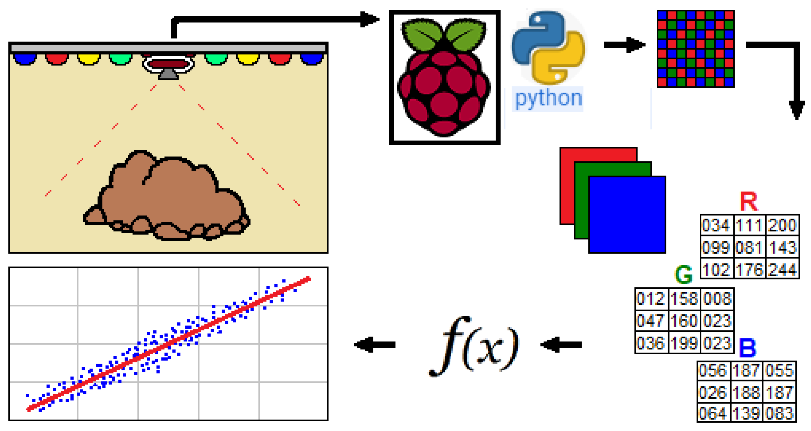
Figure 1 shows the general functioning of the system. The soil samples were placed in front of the LED panel and the camera is centered between a set of LED lamps of five different colors (blue, green, red, yellow and white). When starting the program, it captures images of the same sample on each color of light emitted by the panel.
The initial development of the work was carried out through the construction of the imaging capture structure, which was composed by the LED lights and the NoIR camera inside a box that was duly painted black in order to provide minimal interference in the reflection of the light emitted from the panel. The welding of 5-volt resistors with 330 ohms of resistance was also performed between the LEDs and the GPIO of the Raspberry Pi to prevent the lamps from burning.
Therefore, the assembly becomes simpler, not requiring the multiplexing of the LED lamps.
Figure 2a presents the resulting structure. Regarding the arrangement of the lamps and camera; they were organized in such a way that the incident light was as linear as possible around the camera. So, 30 lamps were installed, six in each wavelength, resulting in a total set of five different wavelengths for analysis.
After welding and assembling the hardware components, tests were carried out to verify the existence of shaded parts on the samples which would affect the performance of the application. Still regarding the cause of shading on the sample, parameters such as disposition and quantity of employed LEDs were essential factors that caused this effect on the images.
Thus, two approaches to solving the problem were possible, the first being an increase in the number of used lamps and the second being the approximation of the lamps, which would result in the modification of its arrangement without changing the quantity.
The first approach—the increase in the number of lamps—was discarded due to the limited availability of resistors and space for the installation of the lamps, as well as the Raspberry Pi GPIO’s ability to support the number of lamps. Therefore, the defined solution was the modification of the arrangement of the LEDs that were already being used, resulting in a distribution in a circular shape.
After changing the arrangement of the lamps there was an improvement in shading; however, this did not fully resolve the issue, so a light deflector was developed in order to avoid the dispersion of the light beam, significantly improving the linearity of the light reflected in the sample, as presented in
Figure 2b.
The application software was developed using Python 2.7 programming language with GPIO libraries to manipulate the Raspberry pins, with the CV2 library referring to the OpenCV to process the images and the PiCamera library to manipulate the camera as well as to capture the images. This software in Python works in the shell terminal of Raspbian GNU/Linux 10.
Figure 3a presents an image that was the result of capturing the soil sample in each beam of light.
OpenCV is a library that can be applied to computer vision and machine learning, offering computational power for admission, detection and image processing. Regarding computer vision, it covers the extraction, manipulation and analysis of images in order to obtain useful information from them to perform a specific task [
34].
The software structure consists of a main class responsible for defining the area of interest before capturing and defining the activation sequence of the LEDs, in addition to the acquisition of the images, one of each color. Finally, the image is cropped in order to follow the area of interest used, in this case 128 × 128 pixels, as shown in
Figure 3b.
We employed the Scikit Learn module with machine learning libraries, more specifically the Partial Least Squares Regression (PLSR) technique. For the correct use of the PLSR method there is a need for a linear data profile, which does not occur with luminance values. Thus, only the histograms of the images were used, as follows:
- 1.
Extraction of the image under the effect of a certain LED color;
- 2.
The image is divided into three histograms;
- 3.
The histograms are concatenated, as well as each of the LED colors.
- 4.
As a result, a CSV file (Comma Separated Values) is generated with all histograms in all LED colors, as illustrated in
Figure 4.
Algorithm 1 shows the procedures developed for the acquisition and processing of images and the prediction of clay results.
| Algorithm 1 Procedure of predicting clay through histogram images. |
Input: Image parameters (ROI) and number of PLSR factors Output: Predicion charts and reporting data - 1:
roi = 128 - 2:
factors = 6 - 3:
leds = [’green’,’red’,’white’,’yellow’,’blue’] - 4:
histograms = [ ] - 5:
for led in leds do - 6:
files = acquireImages(led) - 7:
for file in files do - 8:
histograms.add(processingHistograms(file, roi)) - 9:
end for - 10:
end for - 11:
csv = generateCSV(histograms) - 12:
ref = loadReferences() - 13:
predictionModel = computePLSR(csv, ref, factors) - 14:
reportingData(predictionModel) - 15:
plotingData(predictionModel)
|
The first step consists in acquiring images controlling all LEDs individually using Rapsberry Pi GPIOs. All images are exported in PNG format. The second step creates the red, green and blue histograms from the images obtained in the previous step. The third step transforms the histograms created in the CSV file, joining all 256 color levels of each histogram forming 768 variables per sample. The fourth step computes the prediction model using the PLSR algorithm using the CSV data to correlate with reference data using a specific number of factors. After the model generation reports with predictions and their charts are showed.
All PLSR models were developed based on Daniel Pelliccia’s website, which provides a step by step tutorial on how to build a calibration model using partial least squares regression in Python [
46].
5. Results and Discussions
The calibration models for all sets of histograms were embedded in a Raspberry Pi device. For later comparison of the performance of the models that presented better results, quantifications were made from the figures of merits, both to validate them based on linearity (R2) and on the Root Mean Square Error of Calibration (RMSEC), as well as to evaluate them as calculated by the Root Mean Square Error of Cross Validation (RMSECV).
At first, the addition of three histograms for each LED separately allowed to build the calibration model, thus originating 768 variables. Each model employed a different number of factors according to the best result of RMSECV, as shown in
Table 3.
The white LED generated the best model with the highest R2, estimated at 0.857, and the lowest RMSEC (7.06%). Regarding the RMSECV (13.66%), the value was very close to the yellow LED (13.59%) in this same item.
Then, seeking better results, new modeling was carried out with separate RGB histograms for each LED. In this case, a number of factors equal to 10 were set-up, so that all models could be compared from the same configuration, according to
Table 4.
Comparing the generated values, no model obtained better indexes of figures of merit than the white LED, which presented the highest R2, estimated at 0.857, and the lowest RMSEC (7.06%). In relation to the RMSECV (13.66%), the value was very close to the yellow LED (13.59%) in this same item.
Lastly, a single model was built with all histograms for all LEDs, resulting in 3840 variables. In this case, the model employed a better number of factors, according to the result of RMSECV, as demonstrated in
Table 5. This model generated the best results regarding linearity (R
2 equal to 0.962) and RMSEC (3.66%). About the figure of merit RMSECV, the result was shown to be greater than in the first generated model.
Figure 5 shows the linear performance of this model.
Therefore, the Kennard–Stone algorithm was applied to segregate the samples in a group for calibration and another for validation. From 50 soil samples, the algorithm selected 34 samples for the calibration model and 16 samples for the validation or test model.
Table 6 presents the predicted results from the calibration model and its reference values.
When comparing the results of the calibration model generated in this multispectral LED system with works by different authors, better predictive assessment rates were achieved. Wetterlind et al. in 2015 [
47] obtained an R
2 of 0.76 with an RMSECV of 6.4% and Tümsavaş in 2019 [
8] found an R
2 of 0.91 with an RMSECV of 3.4%, both using the NIR spectroscopy method. The minor RMSECVs of these authors are due to the low sample representativeness. Both focused their experiments on batches of approximately 0.5 km
2, while this work represents various points in Vale do Rio Pardo, Brazil, around 13,255.7 km
2. In addition, other factors such as sensitivity, reproducibility and equipment interference, intrinsic to the method, could also be discussed.
6. Conclusions
This work presented the use of multivariate calibration techniques in soil imaging from a multispectral camera in order to predict the amount of clay present in the samples. Concerning calibration results with low RMSEC values, however, the performance during the prediction could present better indexes.
Clay is one of the required parameters, among others, in order to assess soil fertility. As presented in this work, the concentration of this substance in the soil was quantitatively achieved through a multispectral camera. It was also possible to perceive a great potential in the correlation with the official routine analysis.
As advantages, the methodologies that were developed in this work are simple and maintain the integrity of the samples without the need for methods of greater complexity, presenting relatively low cost. The samples are analyzed in less time without the use of reagents and in a non-invasive way.
The combination of OpenCV and machine learning libraries with a low powered device, as a Raspberry Pi, will allow a wide range of research opportunities in agriculture, more precisely smart farms.
As future work, a larger number of samples could make the model more full bodied, predicting more linear effects due to a larger population. Another approach that could be taken is the generation of smaller calibration groups or range calibration. After a global model estimates an initial result, smaller models, with a restricted calibration range, could improve the accuracy of the sample.
Future research will organize the data collected in Context Histories [
48,
49] to allow pattern recognition [
50], context prediction [
51] and similarity analysis [
52]. These analyses will improve the possibilities to implement intelligent services in the agriculture environments. Finally, the proposed technology can be embedded on equipment used in smart farms such as smart tractors and drones.


 ,
, 


