Abstract
Many regions of the world benefit from heating, ventilating, and air-conditioning (HVAC) systems to provide productive, comfortable, and healthy indoor environments, which are enabled by automatic building controls. Due to climate change, population growth, and industrialization, HVAC use is globally on the rise. Unfortunately, these systems often operate in a continuous fashion without regard to actual human presence, leading to unnecessary energy consumption. As a result, the heating, ventilation, and cooling of unoccupied building spaces makes a substantial contribution to the harmful environmental impacts associated with carbon-based electric power generation, which is important to remedy. For our modern electric power system, transitioning to low-carbon renewable energy is facilitated by integration with distributed energy resources. Automatic engagement between the grid and consumers will be necessary to enable a clean yet stable electric grid, when integrating these variable and uncertain renewable energy sources. We present the WHISPER (Wireless Home Identification and Sensing Platform for Energy Reduction) system to address the energy and power demand triggered by human presence in homes. The presented system includes a maintenance-free and privacy-preserving human occupancy detection system wherein a local wireless network of battery-free environmental, acoustic energy, and image sensors are deployed to monitor homes, record empirical data for a range of monitored modalities, and transmit it to a base station. Several machine learning algorithms are implemented at the base station to infer human presence based on the received data, harnessing a hierarchical sensor fusion algorithm. Results from the prototype system demonstrate an accuracy in human presence detection in excess of ; ongoing commercialization efforts suggest approximately 99% accuracy. Using machine learning, WHISPER enables various applications based on its binary occupancy prediction, allowing situation-specific controls targeted at both personalized smart home and electric grid modernization opportunities.
1. Introduction
1.1. Motivation
It is difficult to overstate the magnitude of the climate crisis that we are facing [1,2,3]. Reducing greenhouse gas emissions is imperative and, while significant strides are being made to convert our electric grid to utilize renewable resources instead of fossil fuels, reducing primary energy consumption remains an important task. Buildings are dominant consumers of electricity and thus offer a large potential for energy reduction. The operation of heating, ventilation, and air conditioning (HVAC) equipment is a substantial contributor to energy consumption in buildings, not all of which occurs when people are in the buildings (and thus will benefit). While commercial and industrial buildings are the biggest consumers of electricity, unnecessary residential energy consumption is an important aspect that needs to be addressed. Eliminating wasted residential building energy use is the primary goal of the presented solution.
Despite technological advances and government legislation that have led to the adoption of more energy efficient buildings and appliances in the United States, newer buildings typically consume the same amount of energy as buildings that were constructed in the 1960s [4]. This means that the technical advances of the last 70 years have not led to a decrease in residential energy consumption (though they may have led to an increase in occupant comfort). The urgency of climate change means that we should consider all possible avenues for energy-use reduction. Within buildings, this means addressing how and when energy is used and not just making improvements to the appliances themselves.
One avenue of reduction would be to air-condition buildings only when it contributes to occupants’ comfort, meaning when they are home or are soon to be home, and studies have shown that by accounting for occupancy use in HVAC operations, residential energy use can be reduced by 15–45% [5,6,7]. While this seems obvious, many homes’ HVAC systems are controlled by simple thermostats and require occupant intervention to change the set point. Because of forgetfulness or an occupant’s desire to always have a comfortable space when they get home, they rarely change the set point of the thermostat and instead always condition the house to the same temperature [8]. Programmable thermostats, which allow you to have multiple “home” and “away” set points, rely on an occupant’s idealized schedule and often do not accurately reflect their actual habits [9]. Furthermore, many occupants find programmable thermostats difficult to use and fail to take advantage of their features [10]. Smart thermostats, which attempt to learn and respond to an occupant’s behaviors and preferences, offer a promising alternative [11,12]; however, usability issues with these devices abound [13], and the energy savings are often much less than promised [14,15]. Thus, accurate occupancy detection, which does not rely on user interaction, has the potential to improve how HVAC systems are operated and to impact building energy use.
In addition to reducing total energy use in buildings, occupancy data from buildings can be used to affect when and how electricity is used, which can help to increase the penetration of renewable energy resources in the electric grid [16]. This can be achieved through mechanisms such as demand response and grid-interactive efficient buildings [17,18]. The increasing electrification of buildings and transportation means that this issue will become even more important in the coming decade [19]. Building operation, at all scales, is one piece of the larger puzzle that needs to be solved to dramatically reduce global greenhouse gas emissions. An often-cited statistics states that buildings consume 40% of all global energy [20], making the reduction of energy use in buildings a significant piece of that puzzle. It is clear that while more research is needed in this field, accurate occupancy detection (and integrated HVAC systems) in homes has the potential to greatly reduce global energy use.
1.2. Design Focus
In this paper, we present a novel technology platform, the Wireless Home Identification and Sensing Platform for Energy Reduction (WHISPER), to offer a possible pathway to realizing residential building energy savings by avoiding energy use when the building is not in use.
The WHISPER system is designed as a next-generation occupancy sensing platform for smart homes, systems, and electric system infrastructure. Occupancy presence detection for smart home control promotes high renewable penetration, grid decarbonization, and associated smart grid applications. Monitoring the human occupancy status supports the growing emphasis on indoor environmental quality (IEQ) and health-in-building applications, while activity-based analytics will enable smart systems at large. WHISPER targets high accuracy as well as low false alarm rates regarding both false negatives (falsely assuming vacancy) and false positives (falsely assuming occupancy), while distinguishing between pets and humans. Its design focus is to achieve substantial energy savings while maintaining wide user acceptance by the purposeful obfuscation of personal information: the system is locally wireless so users can avoid cloud-based approaches and ensure privacy preservation. The WHISPER platform’s hardware and software components, including the hierarchical sensor fusion algorithm, are detailed herein.
While the WHISPER hardware was optimized for residential building applications, the concept has been designed for modularity and extension to most occupant presence monitoring situations; e.g., commercial and industrial applications where occupant detection is necessary. Several hardware sensor nodes deployed in a home communicate with a base station that emits an RF carrier wave and powers the sensor nodes. Without the need for sensor node batteries, the base station both transmits and receives communications. The sensors themselves are of the small peel-and-stick type, comprised of a motherboard and small daughterboard. The daughterboard holds either an image or acoustic energy sensor and relays obfuscated images or filtered acoustic energy signatures back to the base station. The system is extensible to other sensing modalities, including those related to indoor environmental quality (IEQ), security, and occupant health.
The WHISPER software system entails a hierarchical sensor fusion architecture: at a lower level, the individual modalities measured are used to arrive at individual inferences on occupancy using customized machine learning algorithms, including spatial–temporal pattern networks, random forests, and convolutional neural networks. A high-level whole-building fusion algorithm combines the individual inferences and additionally allows for memory terms, since it is not only the instantaneous information but also what happened in the recent past that affects current occupancy status.
A number of applications are feasible and envisioned: (1) home energy efficiency, in an island fashion so that no information is shared, with feasible savings of approximately 100 USD per year [21]; (2) IEQ, including indoor air quality (IAQ) assessment in a post-pandemic world; and (3) grid-interactive efficient buildings. Human presence-driven data analytics constitute WHISPER’s message passing, which seeks to optimally assimilate electrical power system dynamics with slower-moving thermal dynamics and information pertinent to modern, smart home prosumers. The name WHISPER is also an allusion to personal, directed messaging; i.e., it is anticipated that the data analytics associated with WHISPER, beyond achieving energy efficiency and relaying information to occupants, can enable utilities or distribution system operators to flexibly operate the emerging electric system to achieve holistic economic and societal value.
To encapsulate the WHISPER design focus, we offer here a summative preview of the system features as illustrated in Figure 1: (1) a set of sensor nodes, with each sensor element (2) using wireless communication based on digital backscattering and (3) powered by solar panel without the need for batteries. The sensors (4) include image and acoustic energy modalities but can be expanded to any sensor of similarly low power requirements. The (5) ultra-low power backscatter-based sensor network, composed of these sensor nodes, and (6) a sensor fusion algorithm leverage the spatiotemporal interactions of measurements from a residential building to ensure that (7) privacy preservation and low power are possible by collecting camera information in an extremely restricted fashion. (8) Camera gating, which leaves the image sensor nodes off until lower-power, and less obtrusive sensors indicate possible human activity to reduce system power consumption. Furthermore, (9) image sensors can be commanded to capture obfuscated images composed of horizontal and vertical bars that indicate the level and location of activity and require 100× less power than full frame capture from the 10k pixel array, while (10) portions of the image will be collected at higher resolution if human activity has not been ruled out. (11) Human vs. pet discrimination is performed on higher quality sub-images; (12) individual, low-level sensor modality algorithms based on spatiotemporal pattern networks, random forests, and convolutional neural networks will be fed by the various sensor data streams (image, acoustic energy, and environmental features), and a (13) high-level sensor fusion system that ingests data processes instantaneous and past low-level occupancy inferences to achieve high-accuracy occupancy detection.

Figure 1.
Visual representation the WHISPER system and its features.
The main research contribution is the development of a flexible and extensible ultra-low power sensor fusion system that achieves very high occupancy detection with low cost, low maintenance, and high levels of privacy preservation to enable building energy efficiency, healthy indoor environments, and energy flexibility for a modern electric grid system. While a home-level occupancy detection has been the focus of the presented prototype, more granular zone-level occupancy detection is an obvious extension reserved for future development. The system as presented is optimized for maximum privacy preservation by not releasing any personally identifiable information—in fact, any information at all—to third parties.
1.3. Background on Occupancy Detection in Buildings
When analyzing occupancy detection schemes, several distinctions can be made regarding the type of detection scheme and granularity of predictions. One important distinction is between implicit occupancy detection, which involves utilizing existing infrastructure and data streams, and explicit detection, which requires the installation of specialized hardware for the purpose of detecting occupancy. The traditional modes of detection have been explicit, such as passive infrared. Implicit detection is typically cheaper and easier to implement, as no additional infrastructure is needed; however, the capabilities of these systems have traditionally been poor. Recent efforts have been made to improve implicit detection schemes, some of which are described below.
Other distinctions have to do with the resolution, or granularity, with which occupancy is being tracked. The resolution leading to the most diversity in detection schemes is referred to as occupant resolution [22], which has to do with what is being measured. The coarsest grain occupant resolution is a binary occupied/unoccupied status, with the finest grain being the activity of each occupant. Spatial resolution, or the where, can also be considered, as occupancy can potentially be measured for the whole building, individual floors, individual rooms, and even individual work stations, or “zones”, within a room. Traditional occupancy detection has typically been conducted at the room level, though attention is increasingly being applied to work-station level understanding of occupancy in offices. Either of these resolutions can be extrapolated to floor or whole building occupancy detection as well. Finally, the temporal resolution, or when, has to do with how frequently spaces are being sampled and predictions are being made.
Figure 2 gives a visual representation of these different resolutions.

Figure 2.
Representation of different occupancy detection resolution levels across three different dimensions (occupant, temporal, and spatial); from Melfi et al. [22]. Reprinted with permission.
1.3.1. Traditional Methods of Detection
Occupancy detection in buildings has traditionally been performed with passive infrared (PIR) or ultrasonic sensors to control lighting in dual occupancy/vacancy modes. PIR sensors work by detecting heat in the form of infrared radiation that is emitted by all human bodies [23]. The term passive in PIR refers to the fact that these sensors do not emit their own forms of energy but simply sense what is being emitted by occupants. In contrast, ultrasonic sensors utilize a transmitter and receiver system to emit high-frequency sound waves and then measure changes in the signal that is reflected back [24]. Both of these methods are examples of explicit sensing, since they require the installation of dedicated sensing devices.
PIR and ultrasonic sensors are classified as non-terminal sensors, since the occupants being detected do not have to carry a terminal, such as a cell phone or other recognition device. This is in contrast to terminal sensors, such as RFID, where detection is achieved through the use of a sensor or tag that the occupant must carry [23]. Non-terminal systems are inexpensive and easy to install [25]; however, they are generally used at the room-level and can only provide a binary (occupied/vacant) signal, thus they cannot differentiate between one or more occupants in a space [26]. As a result, these systems are usually only used in the context of lighting controls, where lights can be operated in either an occupancy or vacancy mode. Additionally, PIR sensors can only detect a person that is in their direct field of view, which is usually limited, due to gaps in the wedge-shaped detection region of PIR sensors [27]. Further adding to the limitations of PIR is the fact that they work best at detecting moving objects and are not very effective at detecting stationary subjects. Limited movement can result in unwanted false negatives, which leads to lights being turned off when occupants are still in the room [28]. More conservatively programmed sensors will result in fewer false negatives, but the energy-saving benefits of automatic control may be reduced [29].
Because of these limitations, PIR sensors have shown to be most effective at reducing energy use when installed in intermittently occupied spaces, such as stairwells and storage rooms [30], while the savings are generally smaller in larger open spaces, such as offices [22]. Ultrasonic sensors can be more sensitive than PIR sensors [26], providing reduced false negative rates; however, they are also subject to more false positives, as detection can be triggered by factors such as vibrations or air currents [23]. A benefit of ultrasonic sensors over PIR is that signals are reflected off of room surfaces, and so direct line-of-sight to occupants is not necessary [31]; however, they still rely on occupant movement within the space to trigger detection.
1.3.2. Image Detection
Image based systems can be classified as implicit or explicit, depending on whether the image capture technology is already in place. With regards to occupant resolution, cameras are increasingly being used in the context of activity recognition [32], allowing building operators to understand how spaces are being utilized and condition the space accordingly. Recent improvements in computer vision have led to a vast increase in the number and effectiveness of occupancy detection systems involving images [33]. Methods such as histograms of oriented gradients (HOG) and support vector machines (SVM) [34] have made detecting human figures a straightforward problem, especially when the frame and depth-of-view of the camera is not changing. Increases in computational power, leading to improvements in artificial neural networks (ANN), have further led to increases in the detection capabilities of camera-based systems, though these systems can lead to a multitude of privacy concerns for the users [35]. One method of alleviating some of these concerns is to mount cameras directly overhead in doorways [36], which allows occupants to be detected entering or leaving, though not within the space.
While privacy issues are relevant to all forms of occupancy detection, they are of particular concern with image detection systems [37]. Most image-based systems are used in large, public settings, such as shopping malls and office buildings [38]. Generally, in these spaces, privacy for the user is not assumed, and people have grown accustomed to closed circuit cameras (CCTV) in these types of spaces for decades [33]. However, as facial recognition software improves [39], occupants are weary of cameras tracking their movements [40], not only within a space, but between spaces. In smaller public spaces, such as small office buildings and stand-alone shops, security cameras have often been utilized outside the building or in entryways but not frequently deployed within the main spaces. Although in the past, these places have usually relied upon the traditional methods of occupancy detection, such as PIR sensors or fixed occupancy schedules, to control lighting, more privacy-invasive methods are increasingly being used in these types of spaces [41]. The growth of available building data has led to much research into privacy attacks, and into how operators can better protect occupant data [42,43,44].
1.3.3. Other Detection Methods
Another method with the potential for abuse from bad actors is that of occupant tracking [45]. The proliferation of occupants carrying Bluetooth, GPS, NFC, and WiFi-enabled cell phones has made occupant tracking through detection of these devices much easier. When occupants enter a space, their devices are often interacting with the Bluetooth and WiFi systems on site [46]. While these systems do not capture all people in a space, efforts are being made to understand what proportion of people in a space is being captured [47], from which total people counts can be extrapolated. Other methods currently being adopted are based on radio frequency identification (RFID) schemes. These systems, which are most commonly used in office buildings, require occupants to carry an RFID-equipped card on them at all times in a building. These cards are detected by dedicated readers upon entering a building or at different points within a building and can serve as a security feature, as well as performing occupant counting and tracking. Occupant tracking methods are considered implicit, since they generally rely upon infrastructure that is already installed in the space for other uses. An example of one of these schemes is the work done by [22], whereby IP and MAC addresses of employees were tracked inside an office building, showing how many people are connected to the network and inferring total occupancy count from this data.
One area of research that has garnered particular interest recently is that of occupant behavior modeling, as summarized by [48]. These models are usually based on machine learning techniques, such as hidden Markov models (HMM) or k-nearest neighbors [49]. Some of these models take inputs from sensors in the space as indicators of human presence [50], while other methods focus on the arrival and departure patterns of occupants, such as stochastic probability models [51]. Other work has focused on using existing sensor networks to generate belief networks within a space [30].
In addition to behavior modeling to predict occupancy in buildings, research is being done to understand how buildings are being used by occupants and to quantify the relationship between occupancy and energy use. For instance, using presence-based (binary) occupancy sensors in a medium-sized office building, researchers show that a direct linear relationship can be derived between the percentage of space utilization and whole-building energy consumption [52]. An understanding of this relationship can help with energy forecasting needs, which can help to increase the penetration of renewable resources in the electric grid and can provide explanations for the discrepancies between measured and predicted building performance [53].
A large amount of recent work on occupancy detection has focused on sensor fusion techniques [54,55,56,57]. These systems generally utilize a variety of low-cost and low-intrusion sensors, such as CO, relative humidity, and ambient noise. The individual signals from these nodes are fused in some way to provide an overall decision on whether the space is occupied or to provide an estimate of the number of occupants in the space. The novelty in these systems generally comes from the algorithms used to fuse the signals and make the predictions. In [58], the authors used a combination of environmental sensors and contextual information, such as meeting calendars, to predict occupancy on a variety of granularities. Using a hierarchical framework that incorporated k-nearest neighbors and support vector machines, the authors report accuracy up to 95% for binary classification and up to 78% for occupant counting. Using a Gaussian mixture model-based hidden Markov model [59], researchers were able to achieve an average accuracy of 83% when predicting the number of occupants in a mixed-use lecture/office space.
1.3.4. Residential Occupancy Detection
Most of the works cited so far are specific to occupancy detection in commercial spaces. Research on occupancy detection has traditionally been focused on commercial spaces for a number of reasons: the first is that commercial buildings usually have a greater need for automated operations, and greater incentives for energy savings, than residential buildings. Because of the scale of commercial buildings, overuse of electricity has a larger financial impact than in residential buildings, and since the people using electricity are often not the people paying for it in commercial spaces (at least not directly), they might be less likely to prioritize conservation. Furthermore, the logistics of operating an HVAC system in a building serving many people would be very difficult without some sort of automation. Another reason is that commercial spaces may already have the infrastructure necessary for monitoring, such as in the cases of occupant tracking or image detection, and people visiting commercial spaces are more likely to be carrying a cell phone or identification tag while in the building. Furthermore, people’s movements into and out of commercial spaces can be more regular (arrive at 9 a.m., leave at 6 p.m.), and modeling methods, such as stochastic or non-probabilistic modeling, are easier given a larger number of occupants, since individual errors in prediction are smoothed out over many people. Finally, there is the significant issue of privacy. Many of the recent detection techniques utilize occupant observation, such as with cameras, or occupant tracking, such as with RFID sensors. People have traditionally been weary of installing cameras inside their homes, though this might be changing. While occupant tracking systems can potentially be used in home systems, they are hardly foolproof, as they require all occupants to carry enabled devices on them at all times.
Increasingly, smart thermostats are being adopted in homes. These learning thermostats, such as the Nest, use machine learning to observe and learn from an occupants’ behaviors, such as when they leave and come home and what temperature they like at certain times. The makers of these thermostats claim that they lead to 15% or more energy savings [60], but the actual amount saved can depend on a number of external factors and might not be as much as promised [61]. Users also report frustration with the operation of these thermostats and say that they are generally not as good at learning as hoped [62]. Furthermore, researchers have shown that hackers may be able to break into a Nest thermostat [63], and recent hacks of Nest security devices [64] have made people weary about installing connected devices in their homes [65].
Another method of occupancy detection with the potential to be used in homes is that of electrical activity monitoring. Monitoring the electrical activity in a home has traditionally been used in the context of energy disaggregation and non-intrusive load monitoring (NILM), whereby the power consumption patterns of a home are used to determine which appliances are being used at a given time [66]. Recently, the monitoring of high-frequency noise created by switch mode power supplies (SMPS) of modern electronics has proven very successful for event detection and classification in residential contexts [67]. These detection techniques are increasingly being used to determine the occupancy status of a home [68]; however, additional research is needed to show the transferability of these techniques between different home types.
While there are a variety of residential occupancy detection systems available, there are none that are inexpensive and highly accurate while not being privacy invasive. The WHISPER system, described in this manuscript, combines the high accuracy of image or RFID based detection with the privacy preservation aspects of “low-tech” systems such as PIR and is an inexpensive alternative that harnesses advanced machine learning algorithms in a flexible, modular design.
2. Materials and Methods
The overall system development was accomplished by dividing the effort into three tasks: (1) hardware design, which consisted of designing the individual sensor nodes, detection devices, and the base station, along with development of the backscatter communication methodology; (2) sensor fusion algorithm design, which consisted of investigating, choosing, and training individual (low-level) modality level inference algorithms, along with the (high-level) whole-house fusion algorithm; and (3) testing and system integration, which included an initial data collection phase, as well as sensor type and location specification for the sensor nodes. The following section gives details about each of these three development thrusts.
2.1. Sensor Hardware Development
WHISPER’s sensing hardware was designed with three objectives: minimal system maintenance, privacy-preserving edge computing, and modularity to easily adapt to new use cases. The reasoning behind these objectives was three-fold. First, traditional sensor networks require routine maintenance for battery replacement, which is not only a reoccurring cost but also a time-consuming task for users. Second, anonymity favors edge-processing over cloud solutions for cyber-security. Processing the collected sensor data locally eliminates the need to transfer private user data to cloud-based services. Once the user data are processed and anonymized, the resulting insights can be shared with cloud-based services to enable different applications; however, this is secondary to the prime task of WHISPER: local, accurate, and secure modularity for occupancy presence detection. Designing a system that is modular is important when it comes to integrating new sensors in the future to improve performance and potentially adapting the system for applications beyond occupancy presence detection.
To bring the sensing hardware to fruition while meeting these objectives, several challenges were addressed such as developing a low-power hardware design, implementing low-power network communication, and collecting accurate and secure data for insights on building occupancy. In the following subsections, the sensor hardware design and the solutions used to address these challenges and meet WHISPER’s objectives are described.
2.1.1. Backscatter Communication
One of the main challenges in mainstream IoT solutions is the high energy consumption of wireless standards such as WiFi, BLE, or Zigbee. Sensor networks that use these standards consume a significant amount of energy for data transmission and require either a power cable or frequent battery replacement for high-throughput continuous operation [69]. Power cables place a limit on the deployment of the sensor nodes, specifically in the built environment, and the need for frequent battery changes increases the maintenance cost and can negatively impact overall system performance.
Recent advances in ultra-low-power wireless systems have enabled battery-free image capture and even video streaming using backscatter communication [70]. In backscatter communication, the sensor node transfers its data by reflecting the high-frequency signals generated by another device instead of generating the high-frequency signal locally [71,72,73,74]. This significantly reduces the energy required for wireless communication and allows the sensor node to operate solely on the energy harvested from a small solar PV cell. WHISPER employs three devices to enable low-power backscatter data transmission. A TX unit generates the high-frequency carrier signal, a sensor node modulates and reflects the carrier signal to transmit data, and an RX unit demodulates the reflected signal and recovers the sensor data (see Figure 3d). In contrast, in a conventional wireless communication system, only two devices—TX and RX—are required for the communication link.
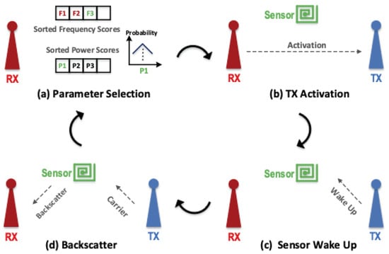
Figure 3.
Sensor node communication cycle: (a) Receiver selects communication parameters, (b) receiver activates transmitter, (c) transmitter wakes up sensor, (d) transmitter generates high-frequency carrier signal, sensor node modulates and reflects carrier signal to transmit data, and receiver unit demodulates reflected signal and recovers sensor data.
2.1.2. Communication Network Design
We introduce two techniques to improve the performance of the backscatter system and extend the operating range to cover more expansive areas such as an apartment or house.
First, a closed-loop tuning system selects the communication parameters (e.g., frequency and TX carrier power) to maximize the backscatter link’s throughput. The propagation loss of wireless signals is frequency dependent. Therefore, the backscatter and TX interference, which operate at separate frequency bands, experience different attenuation levels while propagating toward the RX. Since the backscatter signal carries the data and the TX signal is an interferer, the optimal frequencies for backscatter communications are those with the minimum loss for the backscatter signal and maximum loss for the TX interference. The WHISPER’s closed-loop operation is depicted in Figure 3. The RX unit uses the result of the previous communication attempts to select the best frequency and power level for the carrier signal (Figure 3a). Next, it sends this information to the TX unit, along with the sensor node ID and the command for the sensor node (Figure 3b). Once the TX unit receives the information, it first generates a waveform to wake up the specific sensor node and transfer the command (Figure 3c) and then sends out the carrier signal for backscatter communication. The sensor nodes are in idle mode until the TX unit activates them. Once activated, they respond to the command by sending out one or more backscatter packets (Figure 3d) [75,76].
Further extending the coverage of a backscatter system is possible by using multiple RX and TX base units to form a larger network. Each RX–TX pair can communicate with each sensor node once the node is in its vicinity. The network coverage is first extended by adding more TX units. This solution is suitable for multi-bedroom apartments up to 100 square meters. The data transfer occurs between the RX units and sensor nodes, and TX units are support devices that relay the command to sensor nodes and generate the carrier signal to facilitate the backscatter operation. Adding more TX units, therefore, does not change the system architecture. The RX unit decides which TX unit has the best performance in communicating with each sensor node. Using multiple RX units allows the further extension of the backscatter coverage such that it can cover multi-level residences [76].
To preserve privacy, collected data are processed locally on sensor nodes without transferring data to cloud servers. Raspberry Pi (RPi) single-board computers are utilized to process the collected information. Each RX unit is equipped with an RPi. Since the RX units directly receive the backscatter packets from the sensor nodes, the TX units do not have direct access to the sensor’s data.
2.1.3. Sensor Node Design
WHISPER’s sensor nodes are designed to harvest enough energy from a small solar cell unit to perform sensing and communication tasks. The energy collected from the solar cell is stored on a small rechargeable capacitor, allowing the system to continue operating when ambient light power is unavailable. The sensor nodes must sense and communicate their data efficiently since the energy collected from the solar cell is limited. A low-power ARM Cortex M0+ microcontroller is used in the sensor node design. Each sensor node is equipped with an ultra-low-power wake-up radio based on amplitude modulation, which consumes 3.1 A in listening mode. Each sensor node has a unique 16-bit ID. The microcontroller stays idle, burning a low amount of power until the wake-up radio receives a packet from the TX units with a matching ID. Upon ID detection, the radio generates an interrupt to the microcontroller. Next, the microcontroller transitions into normal mode, reads the received command from the wake-up radio, and responds by sending the required backscatter packets. For backscatter data transmission, the sensor uses an RF switch to modulate the carrier signal.
A modular approach is followed to design the sensor node (Figure 4). The microcontroller unit (MCU), wireless communication units, temperature, humidity, and illuminance (environmental) sensors are placed together to form a basic sensor node. The energy harvesting unit, camera, and acoustic energy sensors are designed as add-on daughterboards that mount on top of the basic sensor node through 5 power and 12 input/output pins. The modular design allows additional sensor types to be added without the redesign of the communication section.
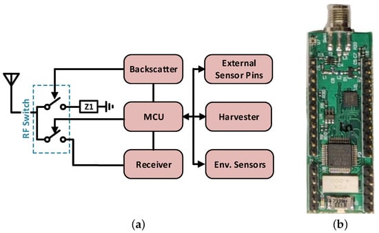
Figure 4.
Sensor node block diagram (a) and basic sensor node board (b).
Camera: A Himax HM01B0 (Himax Technologies, Inc., Tainan City, Taiwan) image sensor running in 120 × 120 pixel mode is utilized. Once a “take-picture” command from the base unit is received, the sensor node’s MCU turns on the image sensor to capture an image that requires 6.05 mJ energy. For data transmission, one image is divided into 12 large sections or 120 small sections, and the base unit can request a large or small section with a dedicated command to complete reading the image. The sensor node consumes 3.82 mJ energy to transmit a complete picture. Once the image is completely transferred from the sensor node to the RX unit, the RX unit sends another take-picture command to restart the process.
Acoustic Energy Sensor: The acoustic energy sensor has three key parts: (1) a microphone, (2) a 16-band filter bank, and (3) a rectifier. The block diagram of the sensor is shown in Figure 5. The sensor uses analog filters to break the audio into 16 frequency bands and then rectifies each band separately to produce an estimate of the power in each band. The energy numbers are sent to the base unit as the inputs of the machine learning algorithms. Like the image sensor, the base unit has to send a command to the sensor to read the energy numbers.
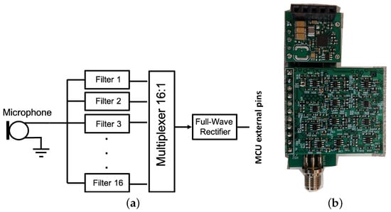
Figure 5.
Block diagram of the acoustic energy sensor (a). An acoustic energy sensor daughter board (bottom) and a harvester board (top) are mounted on a basic sensor node board (b).
The VM1010 microphone used in this work has two operating modes: (1) wake-on-sound and (2) normal. We keep the microphone in wake-on-sound mode, requiring 18 W power, and wait for an acoustic event that generates energy higher than a defined threshold. Once such an event is detected, the processor switches the microphone into normal mode to record the acoustic energy numbers. This feature reduces power consumption by limiting the operation to informative events.
Harvester: Our harvester board shown in Figure 5 uses ambient light to collect energy. Illuminance levels higher than 300 lux provide sufficient energy for sensor nodes. Under conditions when illuminance is below 300 lux, the sensor uses the energy stored on its super capacitor (supercap) for operation. The base unit always monitors the supercap’s voltage of every sensor in the network and adjusts the sensor’s update rate accordingly. In other words, if the supercap’s voltage is decreasing, the base unit requests data from that sensor at a lower rate. As the voltage increases, the base unit increases the update rate. Under conditions when illuminance is less than 300 lux for long periods of time (the base unit is no longer able to adjust the update rate), once the supercap’s voltage hits a low threshold (3.6 V), we cut the power supply and the sensor loses its data. Once the supercap’s voltage hits a high threshold (3.67 V), the sensor becomes active.
2.2. Inference Algorithms
Occupancy inference (i.e., determining whether the space is occupied) is performed in two stages using a hierarchical approach: first, modality level inferencing occurs at a low level, and next, high-level whole-building inferencing aggregation is performed. In the first stage, to get the best modality level occupancy detection results, a variety of models are applied to respective data modalities in order to capture the data patterns that indicate human presence in the house. In the second stage, the detection results from each modality are then aggregated at a high level and fed into an autoregressive logistic regression (ARXLR, described in Section 2.3) model to obtain the final occupancy detection results.
2.2.1. Modality Level Inferences
Environmental Data
The WHISPER system collects three environmental data modalities: indoor air temperature (C), relative humidity (%), and illuminance (lux). In order to learn the relationship between these time series environmental data and the occupancy status, an occupancy detection spatiotemporal pattern network (Occ-STPN) [77] is implemented. In Occ-STPN, a discretization technique known as symbolic dynamic filtering (SDF) is applied to discretize time series data into bins, where each bin represents a range of data values [78] as shown in Figure 6. Each bin is then assigned a designated symbol, which maps the time series data from the continuous domain into the symbolic (discrete) domain, forming symbol sequences [77,79]. Next, time embedding is performed on the symbol sequences in order to encode the historic symbol information into a single state. Figure 7 provides an illustration of this time embedding process and the following steps to construct a state transition matrix.
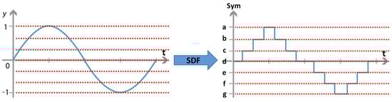
Figure 6.
Results of performing symbolic dynamic filtering on a simple sine graph, which discretizes the data from continuous space to discrete space.
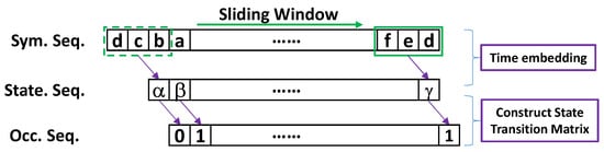
Figure 7.
Time embedding performed on symbol sequence, with sliding window size (depth) of 3 to generate the state sequence, and to construct state transition matrix by capturing the transition between state sequence and occupancy sequence.
For example, if the length of the history or depth (D) of the encoding is three symbols long (i.e., ), a state is then constructed as a sub-array of three symbols from the current timestep t, and two previous timesteps, and , respectively. This time embedding effectively encodes the historic symbols along the symbol sequence to form a state sequence, where each state now contains not only the current information but also the previous timesteps’ information. After obtaining the state sequence, Occ-STPN can now learn the dynamics between an encoded state and the occupancy status and produce a state transition matrix (STM) that maps each state to the occupancy status with associated computed probabilities. After learning the system dynamics, the STM generated by Occ-STPN will output an occupancy status probability from a given state, .
Image Data
For image data, the goal of the inferencing algorithm is to detect the presence of people in the collected image frames. This is accomplished with a custom-trained, state-of-the-art computer vision YOLOv5-based model built on convolutional neural networks, which is deployed on the base station [80]. To train the algorithm, 2500 images from three different locations were collected with the WHISPER system and annotated with occupant location in the image.
Training data consisted of images from various scenarios in an indoor setting, such as different values of room brightness, number of occupants, human postures, occlusions, and occupant distance from camera. This rich variation in the training data helped to improve the model’s robustness to different indoor settings and accustomed the model to grayscale and lower-resolution input images. Camera node sensors can be compared with passive infrared (PIR) motion sensors commonly used in occupancy detection [81,82,83]. As discussed above, most PIR sensors in detection or control systems suffer from two common problems: false positives are common, due to the presence of pets in the residential unit [84], and false negatives are common, when people are relatively still. Using an image sensor node and a well-trained human detection model alleviates these issues, as the system becomes pet-immune and only triggers an occupied status when an actual human is detected in the image, as well as when people are relatively still in the space.
Acoustic Energy Data
The final modality collected by the WHISPER system is acoustic energy (audio) data. The goal of inferencing acoustic energy is to predict the occupancy status by picking up acoustic energy signatures, such as human voices and noises from activities such as cooking, vacuuming, and opening and closing doors. In the WHISPER system, the acoustic energy sensors compliment the use of image sensors by picking up audio at potential blind spots that are not covered by the field of view of the camera.
Although the WHISPER acoustic energy sensor is able to collect audio data, the raw audio is not transferred to the base station, nor is it used directly for occupancy detection purpose. Instead, the audio data goes through a series of processing steps for several purposes, including feature extraction, privacy preservation, and reducing the data communication load. Upon capturing audio, the data pass through a series of band-pass filters as a feature extraction step. The intuition behind band-pass filtering is that different audio noises produce different frequencies; hence, the respective filter bands are excited, producing different frequency signatures.
After the band-pass filtering process, the filtered signal goes through a full-wave rectification and downsampling process before transfer to the base station. These processes ensure the transferred data are non-reconstructable to the original audio, thus eliminating any privacy concerns. The downsampling also reduces the amount of data required to be transferred to the base station. To simplify implementation and ensure privacy preservation, most of the feature extraction steps, including band-pass filtering, full-wave rectification, and downsampling are built-in to the acoustic energy sensor itself as described in Section 2.1.3. In preparation for model training, a total of 1790 audio samples were collected, representing different activities that could indicate human presence, such as talking, cooking, running water, vacuuming, and playing music. These audio samples were used to train a random forest classifier with 100 trees and a depth of 10 to predict if the input data contained indicators of occupancy in the house.
2.3. Sensor Fusion Algorithm
A novel sensor fusion algorithm (SFA) was developed for whole-house occupancy detection, based on an autoregressive logistic regression model with exogenous variables (termed “ARXLR”). Whole-house occupancy was predicted by combining individual modality level occupancy inferences (based on images, noise, and environmental readings) together in the SFA. The proposed algorithm solves two issues: (1) how to combine the different sensor modalities (audio, images, and environmental readings) into one prediction and (2) how to accurately predict occupancy when people are home but no one is active in the monitored areas.
The SFA exploits two aspects of occupant behavior. The first is that people tend to be fairly regular in their schedule regarding leaving home and coming back. While a field of modeling exists which exploits the regularities in peoples’ schedules, referred to as non-probabilistic modeling [85], there are significant drawbacks to these models. These models work by using aggregated historical occupancy data to build a time-of-day probability profile, with each time interval having a probability of home occupancy between 0 and 1. If the probability is above a threshold, the building is predicted to be occupied, while when below the threshold, it is predicted to be vacant [21]. The main limitation of this method is that the accuracy of the model is highly dependent on the training data used, making the transferability of the models poor. However, time-of-day can still be an important predictor of occupancy, and while exact times of arrival and departure vary, most people usually (at least pre-2020) follow similar patterns. Thus, the developed ARXLR algorithm includes time-of-day information and historical patterns, while not relying solely on it, in the same way as a non-probabilistic model.
The second factor exploited is the fact that people do not simply materialize in a room in their house. Whenever a person is asleep (or otherwise quiet) in their bedroom, they must have, at some point prior to that, entered through a doorway, usually walking through the house in the process. People especially tend to be fairly active in the common parts of the home in the evening, while cooking, eating, and socializing. The SFA accounts for this by including a short history of occupancy (on the scale of 4 to 12 h) based on the hypothesis that the occupancy of a home can be reasonably inferred from past occupancy, even when there is no recognizable activity.
2.3.1. Model Framework
The proposed algorithm is an autoregressive logistic regression model with exogenous variables. Autoregressive (AR) refers to the inclusion of previous occupancy predictions as predictors in the model. Exogenous variables (X) are the non-AR terms, namely occupancy probabilities as predicted by the sensor modalities, along with time of day. The overall framework for combining all predictors is logistic regression (LR). As a reminder, the general form of a multi-variate logistic regression model is
where is the model offset or intercept (a scalar), is a vector representing the model coefficients, is a vector of the model predictors, and is shorthand for , or “the probability that y equals 1, given ”. In this case, indicates that the home is occupied and includes previous occupancy predictions as well as instantaneous predictions based on images, audio, time of day, etc. Thus, the left-hand-side of Equation (1) can be read as “the probability that the home is occupied, given a belief in previous home occupancy and readings from instantaneous sources”. By taking the natural logarithm and manipulating both sides, Equation (1) can be transformed to read
By separating the predictors () into autoregressive terms () and exogenous terms ( and ), Equation (2) can be re-written as
where is the vector of exogenous modality coefficients, is the vector of exogenous time-related coefficients, and the autoregressive terms, corresponding to coefficients on the past occupancy predictions, are given by . The vector represents historical occupancy predictions, while is a vector representing the probabilities of occupancy given the instantaneous modalities, and is a vector of containing information on time of day and day of the week. The final form of the equation is given by Equation (4).
where
- = Intercept (model offset);
- = Autoregressive coefficients;
- = Exogenous modality-related coefficients;
- = Exogenous time-related coefficients;
- = Probability of occupation given by audio inference;
- = Probability of occupation given by image inference;
- = Probability of occupation given by temperature inference;
- = Probability of occupation given by relative humidity inference;
- = Probability of occupation given by illuminance inference;
- = Probability of occupation given by inference;
- = Binary weekend–weekday flag (with 0 meaning day is in {Saturday, Sunday});
- = ;
- = ;
- M = Total length of history considered in hours;
- K = Number of time-steps per hour;
- = Occupancy prediction (whole-house) at the current time-step, t;
- = Average of predicted whole-house occupancy m hours in the past.
2.3.2. Algorithm Development
Prior to the development of the WHISPER hardware platform, a preliminary data acquisition system was built to gather high-fidelity occupancy relevant data, along with ground-truth occupancy information, from a number of residential homes. The goal of this was to provide data to start training sensor fusion algorithms before the completion of WHISPER’s hardware development. Data collected in this manner were meant to be representative of what the WHISPER system would collect and included audio, images, and environmental readings.
Data were collected from a total of six homes, each over a consecutive four-week period. Four to five sensor hubs were installed in each home, depending on size, and hubs were placed only in the common areas, such as the living room and kitchen. Data collection and dissemination was overseen by the federal Institutional Review Board (IRB) and protocols were adhered to as laid out in a human subject research (HSR) plan and administered by the IRB. Test subjects were recruited from the testing university’s department of architectural engineering graduate students and faculty in Colorado. Ground-truth occupancy information was collected from the homes via an “if-this-then-that” (IFTTT) software application that was installed on all occupants’ cellular phones, as well as through a paper backup that residents and visitors marked when entering or exiting the home. From these sources of information, a binary occupied/vacant status of the home was calculated for the entire testing period.
Collecting this data was a significant undertaking, and the final dataset was released for public use after processing was performed to remove identifiable characteristics from the audio and images in order to protect the privacy of the residents (Scientific Data, in press).
Data from five of the monitored homes were used to explore various model hyper-parameters, including the number of lag variables to include and the regularization parameter type and value to use. A train/test environment was used to systematically compare the effects of varying different model hyper-parameters. Similar to the method of k-fold cross-validation, the data from each home were split into contiguous subsets of six to eight days in length. Models were then trained on some subset of the groups, while the remainder was reserved for testing. The subsets were contiguous because of the temporal nature of the algorithm; since current predictions relied on past predictions, randomization of the data was not possible, as is commonly done in machine learning tasks. The Python library scikit-learn [86] and the statsmodels package [87] were used for training and testing.
Models were tested in two ways: self and cross. In the self-test scenario, for a home with n subsets, a model was trained on groups and tested on the reserved set. This was repeated for all distinct subsets, meaning that if a home had five subsets, five different models were trained and tested, and testing data were never included in the training set. Model metrics (accuracy, F-scores, TPR, FPR, etc) were aggregated by taking the average over all tested models in a home, and the mean and standard deviation of these values were recorded for that home’s self-test results.
In the cross-test scenario, data from all but one home were combined and used to train a model. The reserved home was then used to test the model. The trained model was deployed one-at-a-time for each subgroup, and the results were averaged to get that home’s cross-test results. Coefficient estimates and model performance metrics were stored for all trained models (self and cross) so that the averages and variance could be compared across homes, testing types, and parameter values.
Three performance metrics were used to evaluate the effects of different parameter values: accuracy, F-score (F), and F-negative (F), which was the standard F-score, but with the coding reversed (defined in Equation (6)).
2.3.3. Lag Values
The autoregressive lag terms are formed by averaging the occupancy value over the lag-hour of interest, where m represents the lag-hour in Equation (4). The number of predictions to average together (K) was dictated by the time-persistency window, , which was the time span (in minutes) over which predictions were made, where . Thus, means that data is aggregated on a 5 min basis, and therefore predictions are averaged each hour. For instance, at 9:00 a.m., a lag of 1 h would be the average of the 12 occupancy predictions from 8:00 a.m. to 8:55 a.m. A lag of two hours would be the average of the 12 occupancy predictions from 7:00 a.m. to 7:55 a.m. Ground-truth occupancy was used to generate the lags in the training phase, and predicted occupancy was used in the testing phase, with the exception of the first M-hour lags in a testing group. Since the algorithm needed occupancy information to begin making predictions, ground truth values for the previous M hours were used to seed the predictions. When evaluating prediction accuracy, the first 24 h were always discarded from every testing scenario, since the inclusion of these would inflate the prediction accuracy.
Since the goal of including lag values was to account for times that people may not have been active (at night), lag values of at least 8 h were considered. To determine the maximum value that would be informative, the idea of the autocorrelation function (ACF) was invoked. The ACF of a time series is the correlation of the time series with time delayed values of itself [88], which in this case meant looking at the correlation of ground truth occupancy readings with previous ground truth occupancy readings.
Shown in Figure 8 are the ACFs for 8 h and 24 h in one of the analyzed homes. The point of interest is where the plots first cross the x-axis, indicating that the ACF = 0. The point that the ACF first crosses the x-axis is where the auto-correlation first equals 0 and can be thought of as the point that useful information is no longer added for a particular time. The plots indicate that, in most cases, a lag of 8 h should likely be sufficiently long to capture information that might inform current occupancy.

Figure 8.
ACF of occupancy in one analyzed home for up-to 8 h (a) and 24 h (b).
Figure 8 shows a pattern that was exhibited in all homes, namely that auto-correlation starts out near unity for short time lags, steadily decreases, crosses the x-axis, and then oscillates between positive and negative values close to zero in a smooth, periodic fashion. Recall that a correlation value of 1 indicates that two variables are perfectly positively correlated, a value of means that they are perfectly negatively correlated, and a value of 0 means that there is no correlation (the relationship between the two variables is random). For instance, the value of the ACF at 12 h shows how much the occupancy at any time is correlated with the occupancy 12 h before that time. It is expected that the ACF would have a cyclic structure with a 24 h period, since people have schedules that are often similar from day to day. Indeed, this is what we see in Figure 8. Local peaks in the ACF occur regularly on 24 h intervals, showing that the occupancy at any time of day is most highly correlated with the occupancy at the same time of day on previous days. The exceptions to this are the values near the lag of 0, which are uniformly the highest, since occupancy is highly correlated on very short time scales.
2.3.4. Regularization
Regularization imposes penalties on the coefficient estimates, such that their values are reduced or eliminated altogether in an effort to arrive at a parsimonious model that optimally balances model complexity with prediction performance. The norm, which imposes a penalty proportional to the sum of absolute values of the coefficients, was used, as it has the benefit of driving some of the parameters to exactly zero, which effectively performs variable selection.
Regularization was introduced to solve two potential issues with the model. The first is that of the transferability of the model. Specifically, it was feared that unregularized models would be overfit to the training data and might not generalize well to other homes. The second issue was that of multicollinearity, which occurs when predictors in a model are correlated with each other, which can make coefficient values less stable, leading to higher variance in the model coefficients. It was known, from the ACF analysis, that there was going to be strong multicollinearity on the lagged variables, particularly on those that represented lags close to each other (such as between 3 and 4 h, or between 6 and 7 h). or lasso (for the least absolute shrinkage and selection operator) regularization was chosen in order to eliminate lags that were redundant and reduce the complexity of the model.
In lasso regression, the researcher specifies the regularization strength, , which controls how much the coefficients are penalized. In the model formulation that was used in this instance, values were specified, such that smaller values meant stronger regularization. Figure 9 show how accuracy, F, and F changed as a function of the regularization parameter. Shown in the graph are the averages of self and cross-testing for all models, along with the standard deviations.
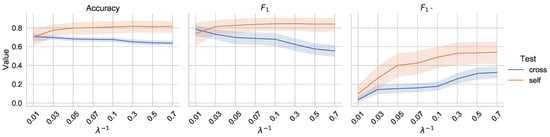
Figure 9.
Performance metrics, with standard deviation, when changing regularization strength.
As can be seen by the figure, there is no “best” value to use. Accuracy was not largely affected by the change, although, as regularization strength decreased ( grew), self-test accuracy increased slightly, and cross-test accuracy decreased slightly. The same pattern is visible in the F score, although the decrease in cross-test score associated with decreased regularization strength is greater. This is likely because of the differences in variable importance from house to house, and the fact that more variables included in the model (as happens when regularization strength decreases) leads to higher variance. This highlights the overfitting problem, as models trained and tested on more similar data (the self-test scenario) generally do well when more predictors are included, but those tested on data that are more dissimilar from training data (cross-test) perform worse. The fact that F increased, in both the self and test cases, as regularization strength decreased, indicates that more of the actual minority class (vacancy states) were accurately classified.
This exploration led to the determination of a final value of for the model, as this represented a good balance between the competing F-scores. This value also retained most of the exogenous coefficients while reducing the number of lag variables included. Using a very small had a large (negative) impact on the F value, even though it only had a small (positive) impact on accuracy. While slightly smaller values like 0.1 showed better F performance, the researchers felt that increasing the F score was important.
2.3.5. Model Coefficients
Based on the parameters chosen through the experiments described (8 h of lags using averages lag values, with of 0.3), a final ARXLR model was trained using balanced subsets of data from all homes.
Note that the raw values of all inputs were between and 1, since they were either probabilities of occupancy (between 0 and 1), outputs of sin or cos functions with amplitude 1 (between −1 and 1), or a weekday indicator variable, which took on values of exactly 0 or 1. Thus, the magnitude of the coefficient is directly related to its impact on the final model decision.
As can be seen in Figure 10, the variables with the largest coefficient estimates are the intercept and the lag of 1 h. Images, audio, temperature, and CO are also relatively large. Most of the coefficient estimates have relatively small standard deviations; however, the intercept, audio, and CO have fairly large standard deviations, indicating that there is quite some variability in the estimates for these values between homes.
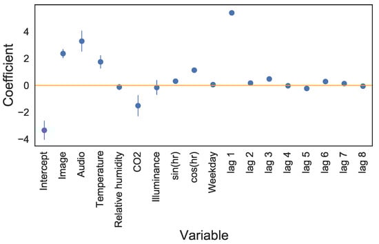
Figure 10.
Model coefficients when considering an 8 h lag, trained with an regularization penalty of . Points show the mean values, and error bars show the standard deviation of the value, across all instrumented homes.
Based on all of the above considerations, final models were generated to compare the ARXLR sensor fusion algorithm against several baseline models. For training the final models, data from all homes were combined into one data set. In order not to bias the model towards a home that had more data, two subgroups from each home were randomly selected (without replacement) to compose the training set. The trained model was then tested on each subgroup to get accuracy, and the results were averaged for each home to get the final results (again, so as not to bias the results towards homes that had more available data). Note that because data from all homes were used to generate the training set, there was no self/test distinction.
Reported in Table 1 are the coefficient estimates from one of the randomly selected training groups. This version, which is representative of the majority of models created, was used to compare against the baselines and as an example to give interpretations of the model coefficients.

Table 1.
Final coefficient estimates and associated statistics for the ARXLR model. Coef. gives the estimated model value and Std. error is the standard error of the estimate. z and p give the z-score and statistical significance of the estimate. The final two columns give the 95% confidence interval for the estimate. Bold variable names are those that are statistically significant at a 5% level (p ≤ 0.05).
2.3.6. Interpretation of Model Coefficients
Given the coefficients in Table 1, the final equation (in the form of the log-odds) can be written as
where the variables are the same as described in Equation (4).
In contrast to interpreting the coefficients of a linear regression model, interpreting the coefficients of a logistic regression model is more complicated; however, the same intuition applies, whereby large magnitude coefficients indicate larger impacts (if the data have been properly normalized or scaled). If the data have not been scaled, however, then large coefficient values may simply be due to small input variables. Similar to linear regression, positive coefficients indicate that an increase in value (in the case of quantitative variables) or presence (in the case of binary indicator variables) of the independent variable will lead to an increase in the response or dependent variable.
For example, the coefficient attached to the probability of occupancy given temperature, , means that a one-unit increase in the probability of occupancy given temperature (as specified by the modality-level inference algorithm) causes the log-odds of occupancy to increase by 1.5 units. Since we are dealing with probabilities (numbers between 0 and 1), it makes more sense to think in terms of a 0.1-unit increase (for instance, probability of occupancy given temperature increasing from 70% to 80%). Since the equation is linear in the log-odds, an increase of 0.1 in probability of occupancy given temperature causes a raw increase in log-odds of occupancy of 0.15. So, if the log-odds in the first case were 1.15, the log-odds after the 0.1-unit change in temperature probability (if nothing else changed) would be 1.3.
This can also be interpreted in terms of the change in odds. Recall that odds are the argument of the logarithm and represent the probability of an event happening divided by the probability of the event not happening:
A one-unit increase in probability of occupancy given temperature () causes the odds of the home being occupied to increase to times what it was at the previous temperature value. A 0.1 unit increase in probability of occupancy given temperature causes the odds of the home being occupied to increase to times the previous value. Given the same example, the odds when would be , and after the increase, the odds would be . The probability of occupancy, , can then be found by transforming back the odds equation:
Meaning that in the first case, , and after the 0.1 unit change in , the probability of occupancy, , is . Because of the non-linearity of the equation, the raw change in seen when switching from would be different from that seen when .
As another example, let us look at the weekday indicator variable: the value of indicates that, all other variables staying constant, the home on a weekday is less likely to be occupied than on a weekend under the same conditions. Specifically, if the conditions are such that the probability of the home being occupied is 90% (i.e., ), then the odds of the home being occupied would be , and the log-odds would be . If all conditions stayed the same, except for it being a weekday, then the log-odds of occupancy would be , the odds would be , and the probability of occupancy would be , or 87%.
3. Results
In this section, the WHISPER system’s performance is demonstrated by testing at different locations including the common areas in a residential apartment and a computer lab. The system’s performance is evaluated by two criteria: (1) the occupancy detection accuracy and (2) the hardware communication and system reliability. Additional tests demonstrated that the sensors are establishing a stable communication with the receiver and transmitter using the backscatter communication technique. The WHISPER system used in testing consisted of one receiver, two transmitters, two image sensor nodes, and two acoustic energy nodes. Each image and acoustic energy node is also coupled with three environmental sensors; i.e., temperature, humidity and illuminance.
3.1. WHISPER System Hardware Evaluation
In this section, we evaluate the performance of our hardware. First, we measure the power consumption of a basic sensor and the update rate of it when a 2 or 17 in solar panel powers up the sensor. Next, we set up the hardware in a hallway to measure the communication range of our backscatter system. Finally, we use our hardware in an apartment to show the wide coverage of the WHISPER system.
3.1.1. Power Consumption
Table 2 lists the power consumption of a basic sensor. This sensor is in idle mode until it receives a command from the base unit. Once the command is received, the sensor records the environmental data and sends them to the base unit. We perform two separate experiments to measure the update rate of our sensor when it uses a small (2 in) and large (17 in) panel for energy harvesting. Our results show when we use the large (small) panel, the sensor collects enough energy to record and transmit environmental data every 0.2 (1) s.
Table 2.
Power analysis for a basic sensor node.
3.1.2. Line-of-Sight Communication Range
We set up the system in a hallway to measure the communication range. In the beginning, the sensor was placed 10 ft far from the TX and RX units (the sensor is in the middle of the TX–RX line). We sent 1000 packets to the RX unit and measured the packet error rate. We repeated this experiment for distances up to 150 ft and recorded the packet error rate (PER) at each point. Figure 11 shows the experiment setup and PER values. Our results show that PER is less than 10% for distances up to 150 (140) ft when the data rate is 31.25 (62.5) Kbps.
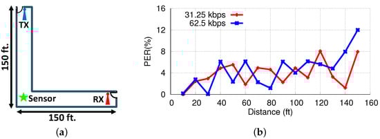
Figure 11.
Range experiment setup (a) and line-of-sight range experiment results (b).
The maximum power was set at 30 dBm (1 W). In our evaluations, we used packets with a 20 byte payload and 2 byte CRC. To receive a packet successfully, all 176 bits needed to be correctly received. If we assume the bits to be independent from each other, the packet error rate (PER) and bit error rate (BER) are related to each other by . Thus, a PER of 10% corresponds to a BER of 0.0598%, which is significantly less than the BER of 1% used in other works.
3.1.3. Coverage
We evaluated the performance of WHISPER in a 800 ft single-bedroom apartment (Figure 12) using one RX unit and three TX units. Similar to the range evaluation, the sensor node transmitted 1000 packets at 18 test points while maintaining a PER of less than 15%. In the floor plan, blue squares, red squares, and green circles are the TX units, RX units, and sensor node test points, respectively. As shown in the updated floor plan, all testing points have a PER less than 15%. PER values change slightly at different locations due to variations in the sensor-to-base unit distance and multipath fading throughout the building.

Figure 12.
Coverage experiment results for 800 ft single-bedroom apartment. Blue squares, red squares, and green circles are the TX units, RX units, and sensor node test points, respectively.
3.2. WHISPER System Evaluation
Testing locations were selected specifically to address potential bias in background settings and occupancy schedules. Each of the locations displayed a different occupancy status profile—the living room primarily showed an occupied status, the kitchen mostly an unoccupied status, and with the lab, a balanced distribution of occupied and unoccupied. The living room was mostly occupied as the occupant spent most of their time working at a desk in the living room. The opposite is true of the kitchen’s occupancy profile, as it is occupied for shorter amounts of time; e.g., during cooking and meal times. Lastly, the lab occupancy profile was relatively balanced with occupied and unoccupied statuses, where the lab’s vacancy correlated with lunchtime and after researchers left the labs around 5 pm. To measure the performance of the system, two metrics were used in the evaluations. Aside from the common accuracy metric, the F-score was used—a metric common for evaluating data with imbalanced classes. The first three rows of Table 3 present the testing results for each aforementioned location. WHISPER was able to achieve an accuracy >95% in all testing locations, which is reflected in Figure 13, where the predicted occupancy status closely matched the true occupancy status. Each location was tested separately for a single day, for up to 10 h, with a 5 min time window for each prediction and up to 2 occupants in each location.
Table 3.
Accuracy and F-score of the WHISPER system testing in different locations.

Figure 13.
Plot of predicted occupancy status against the true occupancy status for each experiment zone. (a) Living room, (b) kitchen, (c) lab.
In addition to testing the detection accuracy of the WHISPER system in each zone, a larger test was also conducted for an extended amount of time to evaluate overall system reliability and detection performance. In this evaluation, the camera and microphones were deployed in both the living room and kitchen of a residential apartment, and the system ran uninterrupted for approximately five days. The distance between the receiver and sensor nodes covered a distance of approximately ∼10 m during the testing.
From Figure 14, it can be seen that the occupied status is detected in the morning when the occupants are active in the common areas (i.e., living room and kitchen), and there is an extended number of vacancy states detected during the night. For this extended five-day experiment, the WHISPER system achieved an accuracy of 95.76% and an F-score of 0.9577. During the experiment, readings were never lost due to communication issues, as the base station was able to determine the best frequency and power level for the sensor nodes upon detecting any reduction in data transfer success rate. The prediction results show that the system can not only provide accurate occupancy detection results but that it can also cover a relatively large area (i.e., two zones simultaneously in this test), and that the hardware performance is stable and reliable when deployed for an extended duration.
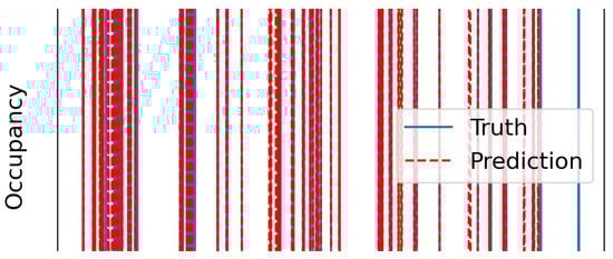
Figure 14.
Predicted occupancy status against true occupancy status for a five-day test that covers both living room and kitchen simultaneously.
3.3. Sensor Fusion Performance
The trained ARXLR sensor fusion algorithm was evaluated on a reserved subset of the training data that were collected from homes, as described in Section 2.3.2. Presented here are the results of the combined ARXLR model tested on each home, as well as performance comparisons between the ARXLR algorithm and different baseline models. Data were captured from six different homes in the internal data acquisition process, but due to difficulties encountered in one home (H4) which led to a limited overall quantity of data being collected, only five of the homes were used to train and test models. The homes that were used to train and evaluate the ARXLR model are referred to as H1, H2, H3, H5, and H6. Models were all evaluated on accuracy, F-score, and F, as described in Section 2.3.2. Recall that F is used when classes are imbalanced, and this gives a particularly critical view when the positively coded variable is underrepresented; i.e., it is highest when positives are correctly identified (high TPR). Similarly, the F is most critical when the negatively coded class is underrepresented (as was the case in most of the homes) and is high when negatives are correctly identified (high TNR). Table 4 gives the performance of the ARXLR algorithm specified in Equation (7) across the three main metrics. Values were calculated for each home and then averaged to get the mean across all homes.
Table 4.
Prediction results of the ARXLR algorithm for each house. Standard deviations are for the different testing groups in each home. Std. dev. in the final row gives the standard deviation of the mean accuracy for all homes.
As can be seen in the table, accuracy was around 85% in all homes, with the exception of home H6, which had much lower accuracy. This pattern was seen across all trials, and there are several possible explanations for the discrepancy. One reason could simply be that H6 had poorer-quality data. There were only four sensor hubs in H6, and on one of them, the audio did not work. It also could be lower because the occupant lived alone and so was not talking with roommates, as occurred in the other houses.
Figure 15 shows one week of predictions in H2, with the probability of occupancy according to the algorithm plotted along with ground truth (0.5 was used as the decision boundary, or cut-off threshold, above which the whole house was predicted to be occupied). As can be seen from the figure, the algorithm performed reasonably well in terms of matching ground truth when the pattern is regular (on the 14th and 15th); however, on the 16th and 17th (a weekend), when the occupant was home for most of the day, the algorithm attempted the same pattern, but then corrected, most likely when it received signals of activity.
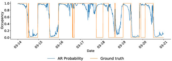
Figure 15.
One week of predictions in home H2, made with the ARXLR model. Blue line shows the probability of occupancy prediction made by the ARXLR algorithms, and orange shows the ground truth (binary) occupancy status.
Figure 16 shows a distribution of how the points were labeled for that week, color-coded according to ground truth. While we do not see the ideal situation, which would be if the two groups were perfectly separated, such that all points above a certain threshold could be labeled as occupied and below labeled as vacant, there is still some reasonable separation between the two groups. The fact that there is a small hump of vacant points around the 0.95 probability (seen behind the blue peak) indicates that a number of vacant points were mislabeled as occupied, while a lack of blue points on the low end indicates that few occupied points were mistakenly labeled as vacant.
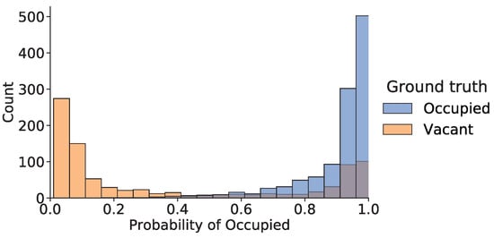
Figure 16.
Distribution depicting how points were classified with the ARXLR model (for one week in H2).
Comparison to Baselines
The performance of the ARXLR model was compared to several different baselines: a minority vote (MV) algorithm; a non-probabilistic method, based only on the time of day; and a version of the ARXLR model that used ground truth occupancy, instead of predicted occupancy, for the lagged values. In addition to the three accuracy metrics previously described, true and false positive and negative rates were calculated for each, as described by Equations (10)–(13).
Minority vote is the incumbent sensor fusion algorithm, implemented in the first iteration of the WHISPER system. This algorithm considers the results of the modality inferences and predicts the whole house to be occupied if any individual modality presents a prediction of occupied. While this algorithm does well at identifying people in direct view or ear-shot of sensors, it does not perform well overnight, when the house is quiet and still.
As can be seen from Table 5, using just acoustic energy and images led to an accuracy only slightly above 50%, meaning the results were not much better than chance. The F and F scores are comparable, and both the true negative and false negative rates were fairly high, indicating the the algorithm over-predicted vacancy and under-predicted occupancy. This is in line with what would be expected if using just the zone indicators, as audio and images are good at detecting when a person is in the same zone as the sensor, but not otherwise.
Table 5.
Results of the three baseline algorithms compared with the ARXLR algorithm. Reported are three accuracy metrics, along with the change in that metric (difference between ARXLR and the baseline). Ground truth is the ARXLR algorithm, using ground truth occupancy.
The non-probabilistic (NP) model showed quite good results, and in most cases performed similarly to the ARXLR algorithm. Recall that NP models generate likelihoods of occupancy based on historically observed occupancy states, which give a predicted probability of occupancy at any time of day. Times with a probability above some threshold are classified as occupied, and those below the threshold are classified as vacant. These models are called non-probabilistic, or deterministic, since there is no chance or randomness in the final decision—it is based only on the time of day (and possibly the day of the week).
In all metrics, other than FNR, the ARXLR algorithm outperformed the NP model. The best performance increase was in F, where the ARXLR model showed a performance twice as good as the NP model; however, the raw values for F, in both cases, were still very low, indicating that both the ARXLR and NP models had a difficult time correctly identifying vacant states. The high false positive rates (or low true negative rates, as TNR 1 − FPR) further show that both models had a difficult time correctly identifying vacant (negative) states, although ARXLR did a better job on both counts than the NP model.
A possible reason for the increased performance over the NP model lies in ability of ARXLR to take in instantaneous state information. While both models rely heavily on historical patterns (NP exclusively, and ARXLR through the and terms), ARXLR can have its belief due to time-of-day overwritten by activity in the space, as we see on the 18th, in Figure 15. When trained on aggregated information from different homes, the NP model does an acceptable job of predicting this occupant’s patterns and does not seem to do much better when trained on its own data. This shows that, if a wealth of ground truth information is available for training, a non-probabilistic could potentially perform well; however, when transferring a model to a new home, with some (indirect) feedback from the occupants, the inclusion of instantaneous readings can serve to train the model as it is used.
As a final comparison, ARXLR was compared to a version of itself that uses ground truth occupancy for the lagged values. This represents a best-case scenario for ARXLR and, as expected, had very good performance. The comparison shows how, with perfect historical predictions, the algorithm could perform very well. While perfect historical predictions are unattainable, this shows how increasing the predictive accuracy of the model has compounding effects, because of its high reliance on the past predictions. The (relatively) high false positive rate of the ground truth model indicates that most of the prediction errors are when the algorithm believes the house is occupied but it is actually vacant.
3.4. Energy Savings Potential
The US funding agency ARPA-E estimated that including reliable occupancy information in the operation of HVAC systems can lead to energy savings up to 30% over baseline usage [89], while Panchabikesan et al. estimate the savings at 5–25% [90]. Turley et al. showed that including occupancy information in a model predictive control (MPC) strategy in a home can result in savings of 13% [21]—a goal that appears to be more attainable than the funding agency’s aspirational target of 30%.
4. Discussion
WHISPER’s primary focus has been presence detection for residential applications, primarily for homes where there is adequate savings potential in binary on/off decision making or through the modulation of set points. Its strength lies in optimizing the trade-offs associated with energy or power, carbon impact or emissions, and time-dependent comfort criteria. Since comfort criteria are subjective (although quantifiable), the objective function may change according to user scenario.
The crucial fact remains that human experiences and their (indirect) manipulation of the WHISPER system will ultimately determine its benefits. That is, savings from HVAC temperature setpoint modulation in conjunction with battery dispatch (electric vehicle or home scale) are bounded by the proportion of time spent in occupied versus unoccupied states (along with pricing or other incentives), as well as by weather—the other main, uncontrollable forcing function defining any window of opportunity for building energy efficiency technologies.
4.1. System Extension
Numerous extensions to the task of residential building energy conservation through binary occupancy detection present themselves, as briefly outlined below.
4.1.1. Additional Sensor Modalities
Sensing of CO is feasible and was demonstrated on early versions of WHISPER’s daughterboard design; likewise, high-frequency electromagnetic interference (EMI) sampling was demonstrated with the goal of adaptive-rate power quality sampling for grid integration (detailed below) in conjunction with environment sampling. The current iteration of WHISPER does not utilize these additional sensor modalities due to cost constraints. However, future research may seek to quantify occupancy events from both the high-frequency electrical waveform perspective and the human temporal dynamics perspective, such as how a human activity, such as cooking, impacts the space. This information could be used for time-synchronous grid-interactive efficient buildings with labeled activity events.
4.1.2. Occupancy Counting
Extending WHISPER’s functionality to move beyond occupancy presence into counting may be achieved through WHISPER’s image sensor node. Popular image processing packages already include subroutines for (human) figure, posture, and face detection, which could be enabled through straightforward coupling to WHISPER’s codebase. However, these elements were considered out-of-scope as driven by constraints for privacy; i.e., integrating high-resolution imagery from a range of commercially available cameras is feasible but begs the question as to whether end users desire to be recorded.
4.2. Non-Energy Benefits
Human engagement with smart devices is an evolving topic, with end users spanning a range of technology acceptance levels. From a conceptual standpoint, WHISPER fundamentally monitors and contributes to the understanding of humans’ engagement with devices in a smart home. Although countless smart device integrations are feasible, WHISPER’s focus is the interface between humans and smart homes for message bus signaling and automating smart grid engagement.
4.2.1. Health Care
Monitoring health care environments for notable events is attracting interest due to its trivial cost in comparison to dedicated, professional health care. As combined with health data from wearables, image sensors in smart homes could be used as part of healthcare monitoring systems, such as the SPHERE IoT network [91]. Additionally, the longitudinal monitoring of human activity in a home may help diagnose trends, such as the onset or escalation of Parkinson’s disease [92].
4.2.2. Security
Security systems can benefit from WHISPER in two ways: (1) as a component of existing security systems or (2) with further development of WHISPER to distinguish between welcome and unwelcome occupants, similar to the pet detection problem, but likely requiring more sophistication to distinguish user type. As such, WHISPER’s inherent security features could be expanded to door and window sensors, traditional IoT cameras, and associated devices. Crucial to the future development of WHISPER are its machine learning capabilities, which could be expanded to include time-dependent activity identification, allowing for whole-home or zone-specific security; e.g., exposure to critical infrastructure or passage through unauthorized spaces.
4.2.3. Indoor Environmental Quality
Indoor environmental quality (IEQ) encapsulates the majority of the empirical data that one might capture to assess a given occupant’s satisfaction with their ambient environment, well beyond simple thermal comfort assessment. In this context, WHISPER may be expanded to interface with smart devices to display not only the binary occupancy state but the instantaneous assessment of IEQ including thermal, indoor air quality, acoustic, olfactory, and visual comfort dimensions. This would require the IEQ attributes to be included in the machine learning framework of WHISPER such that IEQ may be estimated at a higher fidelity. Quantifying and tracking IEQ represents a more valuable and informative characterization of occupied spaces, offering feedback to architects, building design engineers, owners, and operators.
4.3. Conclusions
WHISPER is an end-to-end system for human occupancy detection that can be leveraged to improve the energy efficiency of homes and buildings. Ultra low-power sensor nodes are utilized to collect and wirelessly transmit data to a base station. WHISPER’s base station is designed to perform edge computing and couple sensor data with machine learning to provide valuable insights on human presence and, in turn, provide energy savings and capabilities for smart electric grid participation. Our proposed system preserves the residents’ privacy by relying on low-resolution image sensors and acoustic sensors that report lossy energy-by-frequency audio (uninterpretable) and uses a local wireless network that does not rely on any cloud platform.
The WHISPER hardware platform builds upon novel technologies, including backscatter communication and customized machine learning algorithms integrated in a hierarchical sensor fusion algorithm, to enable a seamless sensing system that requires little to no maintenance and provides accurate predictions on building occupant presence. WHISPER was deployed in multiple homes for approximately one week and demonstrated a detection accuracy of more than . Finally, we highlight several future research directions for WHISPER in healthcare, security, and indoor environmental quality.
Author Contributions
Conceptualization, G.H., S.S., J.S. and A.F.; methodology, G.H., S.S., J.S. and A.F.; software, M.J., S.Y.T., M.K., A.S., H.S., Z.K. and J.G.; validation, M.J., S.Y.T., M.K. and A.S.; formal analysis, M.J. and S.Y.T.; investigation, M.J., S.Y.T., M.K., A.S., H.S., Z.K. and J.G.; resources, G.H., S.S., J.S. and A.F.; data curation, M.J., S.Y.T. and J.G.; writing—original draft preparation, M.J., S.Y.T., M.K., A.S., H.S. and Z.K.; writing—review and editing, G.H., S.S., J.S. and A.F.; visualization, M.J., S.Y.T., M.K. and A.S.; supervision, G.H., S.S., J.S. and A.F.; project administration, G.H., S.S., J.S. and A.F.; funding acquisition, G.H., S.S., J.S. and A.F. All authors have read and agreed to the published version of the manuscript.
Funding
This work was authored in part by the National Renewable Energy Laboratory, operated by the Alliance for Sustainable Energy, LLC, for the U.S. Department of Energy (DOE) under Contract No. DE-AR0000938. Funding provided by U.S. Department of Energy, Advanced Research Projects Agency–Energy (ARPA-E). The views expressed in the article do not necessarily represent the views of the DOE or the U.S. Government. The U.S. Government retains and the publisher, by accepting the article for publication, acknowledges that the U.S. Government retains a nonexclusive, paid-up, irrevocable, worldwide license to publish or reproduce the published form of this work, or allow others to do so, for U.S. Government purposes.
Institutional Review Board Statement
The study was conducted according to the guidelines of the Declaration of Helsinki and approved by the Institutional Review Board of the University of Colorado Boulder (protocol: 18-0658; approved: 17 December 2018).
Informed Consent Statement
Informed consent was obtained from all subjects involved in the study.
Data Availability Statement
The data presented in this study are available on request from the corresponding author.
Conflicts of Interest
The authors declare no conflict of interest. The funders had no role in the design of the study; in the collection, analyses, or interpretation of data; in the writing of the manuscript, or in the decision to publish the results.
References
- Sippel, S.; Meinshausen, N.; Fischer, E.M.; Székely, E.; Knutti, R. Climate change now detectable from any single day of weather at global scale. Nat. Clim. Chang. 2020, 10, 35–41. [Google Scholar] [CrossRef]
- Hoegh-Guldberg, O.; Jacob, D.; Taylor, M.; Bolaños, T.G.; Bindi, M.; Brown, S.; Camilloni, I.A.; Diedhiou, A.; Djalante, R.; Ebi, K.; et al. The human imperative of stabilizing global climate change at 1.5 °C. Science 2019, 365, eaaw6974. [Google Scholar] [CrossRef] [PubMed] [Green Version]
- IPCC. Climate Change and Land: An IPCC Special Report on Climate Change, Desertification, Land Degradation, Sustainable Land Management, Food Security, and Greenhouse Gas Fluxes in Terrestrial Ecosystems; IPCC: Geneva, Switzerland, 2019; pp. 1–864. [Google Scholar]
- Berry, C.; Lawson, G.; Woodward, M. Highlights from the 2015 RECS: Energy Consumption, Expenditures, and End-Use Modeling; Technical Report; U.S. Energy Information Administration: Washington, DC, USA, 2018.
- Lu, J.; Sookoor, T.; Srinivasan, V.; Gao, G.; Holben, B.; Stankovic, J.; Field, E.; Whitehouse, K. The Smart Thermostat: Using Occupancy Sensors to Save Energy in Homes. In Proceedings of the 8th ACM Conference on Embedded Networked Sensor Systems; SenSys ’10; Association for Computing Machinery: New York, NY, USA, 2010; pp. 211–224. [Google Scholar] [CrossRef]
- Gao, G.; Whitehouse, K. The Self-Programming Thermostat: Optimizing Setback Schedules Based on Home Occupancy Patterns. In Proceedings of the First ACM Workshop on Embedded Sensing Systems for Energy-Efficiency in Buildings; BuildSys ’09; Association for Computing Machinery: New York, NY, USA, 2009; pp. 67–72. [Google Scholar] [CrossRef]
- Soltanaghaei, E.; Whitehouse, K. WalkSense: Classifying Home Occupancy States Using Walkway Sensing. In Proceedings of the 3rd ACM International Conference on Systems for Energy-Efficient Built Environments; BuildSys ’16; Association for Computing Machinery: New York, NY, USA, 2016; pp. 167–176. [Google Scholar] [CrossRef] [Green Version]
- Pritoni, M.; Meier, A.K.; Aragon, C.; Perry, D.; Peffer, T. Energy efficiency and the misuse of programmable thermostats: The effectiveness of crowdsourcing for understanding household behavior. Energy Res. Soc. Sci. 2015, 8, 190–197. [Google Scholar] [CrossRef] [Green Version]
- Peffer, T.; Pritoni, M.; Meier, A.; Aragon, C.; Perry, D. How people use thermostats in homes: A review. Build. Environ. 2011, 46, 2529–2541. [Google Scholar] [CrossRef] [Green Version]
- Meier, A. How people actually use thermostats. In Proceedings of the American Council for an Energy-Efficient Economy Conference, ACEEE (2010), Sacramento, CA, USA, 14–17 November 2010. [Google Scholar]
- Ayan, O.; Turkay, B. Smart Thermostats for Home Automation Systems and Energy Savings from Smart Thermostats. In Proceedings of the 2018 6th International Conference on Control Engineering Information Technology (CEIT), Istanbul, Turkey, 25–27 October 2018; pp. 1–6. [Google Scholar] [CrossRef]
- Stopps, H.; Touchie, M.F. Reduction of HVAC system runtime due to occupancy-controlled smart thermostats in contemporary multi-unit residential building suites. IOP Conf. Ser. Mater. Sci. Eng. 2019, 609, 062013. [Google Scholar] [CrossRef] [Green Version]
- Miu, L.M.; Mazur, C.M.; van Dam, K.H.; Lambert, R.S.; Hawkes, A.; Shah, N. Going smart, staying confused: Perceptions and use of smart thermostats in British homes. Energy Res. Soc. Sci. 2019, 57, 101228. [Google Scholar] [CrossRef]
- Pritoni, M.; Woolley, J.M.; Modera, M.P. Do occupancy-responsive learning thermostats save energy? A field study in university residence halls. Energy Build. 2016, 127, 469–478. [Google Scholar] [CrossRef]
- Bustamante, S.; Castro, P.; Laso, A.; Manana, M.; Arroyo, A. Smart thermostats: An experimental facility to test their capabilities and savings potential. Sustainability 2017, 9, 1462. [Google Scholar] [CrossRef] [Green Version]
- Wang, J.; Garifi, K.; Baker, K.; Zuo, W.; Zhang, Y.; Huang, S.; Vrabie, D. Optimal Renewable Resource Allocation and Load Scheduling of Resilient Communities. Energies 2020, 13, 5683. [Google Scholar] [CrossRef]
- Garifi, K.; Baker, K.; Touri, B.; Christensen, D. Stochastic Model Predictive Control for Demand Response in a Home Energy Management System. In Proceedings of the 2018 IEEE Power Energy Society General Meeting (PESGM), Portland, OR, USA, 5–9 August 2018; pp. 1–5. [Google Scholar] [CrossRef]
- Roth, A.; Reyna, J. Grid-Interactive Efficient Buildings Technical Report Series: Whole-Building Controls, Sensors, Modeling, and Analytics; Technical Report; USDOE Office of Energy Efficiency and Renewable Energy (EERE); Energy Efficiency Office and National Renewable Energy Laboratory (NREL): Washington, DC, USA, 2019. [Google Scholar] [CrossRef]
- Blonsky, M.; Nagarajan, A.; Ghosh, S.; McKenna, K.; Veda, S.; Kroposki, B. Potential Impacts of Transportation and Building Electrification on the Grid: A Review of Electrification Projections and Their Effects on Grid Infrastructure, Operation, and Planning. Curr. Sustain. Energy Rep. 2019, 6, 169–176. [Google Scholar] [CrossRef]
- U.S. Energy Information Administration. Monthly Energy Review. Available online: https://www.eia.gov/totalenergy/data/monthly/archive/00352104.pdf (accessed on 2 December 2021).
- Turley, C.; Jacoby, M.; Pavlak, G.; Henze, G. Development and evaluation of occupancy-aware HVAC control for residential building energy efficiency and occupant comfort. Energies 2020, 13, 5396. [Google Scholar] [CrossRef]
- Melfi, R.; Rosenblum, B.; Nordman, B.; Christensen, K.; Nordman, B.; Meier, A. Measuring Building Occupancy Using Existing Network Infrastructure. In Proceedings of the 2011 International Green Computing Conference and Workshops, Orlando, FL, USA, 25–28 July 2011; pp. 1–8. [Google Scholar] [CrossRef] [Green Version]
- Labeodan, T.; Zeiler, W.; Boxem, G.; Zhao, Y. Occupancy measurement in commercial office buildings for demand-driven control applications—A survey and detection system evaluation. Energy Build. 2015, 93, 303–314. [Google Scholar] [CrossRef] [Green Version]
- Stolshek, J.D.; Koehring, P.A. Ultrasonic Technology Provides for Control of Lighting. IEEE Trans. Ind. Appl. 1984, IA-20, 1564–1572. [Google Scholar] [CrossRef]
- Yang, D.; Xu, B.; Rao, K.; Sheng, W. Passive infrared (PIR)-based indoor position tracking for smart homes using accessibility maps and a-star algorithm. Sensors 2018, 18, 332. [Google Scholar] [CrossRef] [Green Version]
- Caicedo, D.; Pandharipande, A. Ultrasonic arrays for localized presence sensing. IEEE Sens. J. 2012, 12, 849–858. [Google Scholar] [CrossRef]
- Guo, X.; Tiller, D.K.; Henze, G.P.; Waters, C.E. The performance of occupancy-based lighting control systems: A review. Light. Res. Technol. 2010, 42, 415–431. [Google Scholar] [CrossRef]
- Shen, W.; Newsham, G.; Gunay, B. Leveraging existing occupancy-related data for optimal control of commercial office buildings: A review. Adv. Eng. Inform. 2017, 33, 230–242. [Google Scholar] [CrossRef] [Green Version]
- Hobson, B.W.; Lowcay, D.; Gunay, H.B.; Ashouri, A.; Newsham, G.R. Opportunistic occupancy-count estimation using sensor fusion: A case study. Build. Environ. 2019, 159, 106154. [Google Scholar] [CrossRef]
- Dodier, R.H.; Henze, G.P.; Tiller, D.K.; Guo, X. Building occupancy detection through sensor belief networks. Energy Build. 2006, 38, 1033–1043. [Google Scholar] [CrossRef]
- Haq, M.A.U.; Hassan, M.Y.; Abdullah, H.; Rahman, H.A.; Abdullah, M.P.; Hussin, F.; Said, D.M. A review on lighting control technologies in commercial buildings, their performance and affecting factors. Renew. Sustain. Energy Rev. 2014, 33, 268–279. [Google Scholar] [CrossRef]
- Liu, X.; Ghosh, P.; Ulutan, O.; Manjunath, B.S.; Chan, K.; Govindan, R. Caesar: Cross-camera complex activity recognition. In Proceedings of the 17th Conference on Embedded Networked Sensor Systems, SenSys 2019, New York, NY, USA, 10–13 November 2019; pp. 232–244. [Google Scholar] [CrossRef]
- Tsakanikas, V.; Dagiuklas, T. Video surveillance systems-current status and future trends. Comput. Electr. Eng. 2018, 70, 736–753. [Google Scholar] [CrossRef]
- Dalal, N.; Triggs, B.; Schmid, C.; Dalal, N.; Triggs, B.; Schmid, C.; Detection, H.; Oriented, U. Human Detection using Oriented Histograms of Flow and Appearance. In Proceedings of the European Conference on Computer Vision (ECCV ’06), Graz, Austria, 7–13 May 2006; pp. 428–441. [Google Scholar]
- Howard, B.; Acha, S.; Shah, N.; Polak, J. Implicit Sensing of Building Occupancy Count with Information and Communication Technology Data Sets. Build. Environ. 2019, 157, 297–308. [Google Scholar] [CrossRef]
- Sun, K.; Zhao, Q.; Zou, J. A review of building occupancy measurement systems. Energy Build. 2020, 216, 109965. [Google Scholar] [CrossRef]
- Caleb Sangogboye, F.; Jia, R.; Hong, T.; Spanos, C.; Baun Kjærgaard, M. A framework for privacy-preserving data publishing with enhanced utility for cyber-physical systems. ACM Trans. Sens. Netw. 2018, 14, 1–22. [Google Scholar] [CrossRef] [Green Version]
- Beymer, D. Person counting using stereo. In Proceedings of the Workshop on Human Motion, Austin, TX, USA, 7–8 December 2000; pp. 127–133. [Google Scholar] [CrossRef]
- Yang, C.E.; Shen, Y.T.; Liao, S.H. Integration of Real-time Facial Recognition and Visualization in BIM. In Proceedings of the 2020 IEEE Eurasia Conference on IOT, Communication and Engineering (ECICE), Yunlin, Taiwan, 23–25 October 2020; pp. 243–245. [Google Scholar] [CrossRef]
- Wang, X.; Tague, P. Non-Invasive User Tracking via Passive Sensing: Privacy Risks of Time-Series Occupancy Measurement. In Proceedings of the 2014 Workshop on Artificial Intelligent and Security Workshop; AISec ’14; Association for Computing Machinery: New York, NY, USA, 2014; pp. 113–124. [Google Scholar] [CrossRef]
- Ahmad, J.; Larijani, H.; Emmanuel, R.; Mannion, M.; Javed, A. Occupancy detection in non-residential buildings—A survey and novel privacy preserved occupancy monitoring solution. Appl. Comput. Inform. 2018, 1–9. [Google Scholar] [CrossRef]
- Schwee, J.H.; Sangogboye, F.C.; Kjærgaard, M.B. Evaluating Practical Privacy Attacks for Building Data Anonymized by Standard Methods. In Proceedings of the 2nd InternationalWorkshop on Security and Privacy for the Internet-of-Things (IoTSec), London, UK, 15 November 2019; pp. 11–14. [Google Scholar]
- Jia, R.; Dong, R.; Sastry, S.S.; Spanos, C.J. Privacy-enhanced architecture for occupancy-based HVAC Control. In Proceedings of the 8th International Conference on Cyber-Physical Systems, Pittsburgh, PA, USA, 18–21 April 2017; pp. 177–186. [Google Scholar] [CrossRef] [Green Version]
- Pappachan, P.; Degeling, M.; Yus, R.; Das, A.; Bhagavatula, S.; Melicher, W.; Naeini, P.E.; Zhang, S.; Bauer, L.; Kobsa, A.; et al. Towards Privacy-Aware Smart Buildings: Capturing, Communicating, and Enforcing Privacy Policies and Preferences. In Proceedings of the 2017 IEEE 37th International Conference on Distributed Computing Systems Workshops (ICDCSW), Atlanta, GA, USA, 5–8 June 2017; pp. 193–198. [Google Scholar] [CrossRef]
- Raij, A.; Ghosh, A.; Kumar, S.; Srivastava, M. Privacy risks emerging from the adoption of innocuous wearable sensors in the mobile environment. In Proceedings of the ACM CHI Conference on Human Factors in Computing System, Vancouver, BC, Canada, 7–12 May 2011; pp. 11–20. [Google Scholar] [CrossRef]
- Nicolai, T.; Kenn, H. About the relationship between people and discoverable Bluetooth devices in urban environments. In Proceedings of the Mobility Conference 2007—The 4th Int. Conf. Mobile Technology, Applications and Systems, Mobility 2007, Incorporating the 1st Int. Symp. Computer Human Interaction in Mobile Technology, IS-CHI 2007, Singapore, 10–12 September 2007; pp. 72–78. [Google Scholar] [CrossRef]
- Park, J.Y.; Mbata, E.; Nagy, Z. Good to see you again: Capture and recapture method on mobile devices to estimate occupancy profiles. In Proceedings of the BuildSys 2019—The 6th ACM International Conference on Systems for Energy-Efficient Buildings, Cities, and Transportation, New York, NY, USA, 13–14 November 2019; pp. 145–148. [Google Scholar] [CrossRef]
- Yang, J.; Santamouris, M.; Lee, S.E. Review of occupancy sensing systems and occupancy modeling methodologies for the application in institutional buildings. Energy Build. 2016, 121, 344–349. [Google Scholar] [CrossRef]
- Saha, H.; Florita, A.R.; Henze, G.P.; Sarkar, S. Occupancy sensing in buildings: A review of data analytics approaches. Energy Build. 2019, 188–189, 278–285. [Google Scholar] [CrossRef]
- Huchuk, B.; Sanner, S.; O’Brien, W. Comparison of machine learning models for occupancy prediction in residential buildings using connected thermostat data. Build. Environ. 2019, 160, 106177. [Google Scholar] [CrossRef]
- Page, J.; Robinson, D.; Morel, N.; Scartezzini, J.L. A generalised stochastic model for the simulation of occupant presence. Energy Build. 2008, 40, 83–98. [Google Scholar] [CrossRef]
- Mosiman, C.; Henze, G.; Els, H. Development and Application of Schema Based Occupant-Centric Building Performance Metrics. Energies 2021, 14, 3513. [Google Scholar] [CrossRef]
- van Dronkelaar, C.; Dowson, M.; Burman, E.; Spataru, C.; Mumovic, D. A Review of the Energy Performance Gap and Its Underlying Causes in Non-Domestic Buildings. Front. Mech. Eng. 2016, 1, 17. [Google Scholar] [CrossRef] [Green Version]
- Chen, Z.; Jiang, C.; Xie, L. Building occupancy estimation and detection: A review. Energy Build. 2018, 169, 260–270. [Google Scholar] [CrossRef]
- Arvidsson, S.; Gullstrand, M.; Sirmacek, B.; Riveiro, M. Sensor Fusion and Convolutional Neural Networks for Indoor Occupancy Prediction Using Multiple Low-Cost Low-Resolution Heat Sensor Data. Sensors 2021, 21, 1036. [Google Scholar] [CrossRef] [PubMed]
- Kampezidou, S.I.; Ray, A.T.; Duncan, S.; Balchanos, M.G.; Mavris, D.N. Real-time occupancy detection with physics-informed pattern-recognition machines based on limited CO2 and temperature sensors. Energy Build. 2021, 242, 110863. [Google Scholar] [CrossRef]
- Rueda, L.; Agbossou, K.; Cardenas, A.; Henao, N.; Kelouwani, S. A comprehensive review of approaches to building occupancy detection. Build. Environ. 2020, 180, 106966. [Google Scholar] [CrossRef]
- Khan, A.; Plötz, T.; Nicholson, J.; Mellor, S.; Jackson, D.; Ladha, K.; Ladha, C.; Hand, J.; Clarke, J.; Olivier, P. Occupancy monitoring using environmental & context sensors and a hierarchical analysis framework. In Proceedings of the BuildSys ’14: 1st ACM Conference on Embedded Systems for Energy-Efficient Buildings, Memphis, TN, USA, 5–6 November 2014; pp. 90–99. [Google Scholar] [CrossRef]
- Dong, B.; Lam, K.P. Building energy and comfort management through occupant behaviour pattern detection based on a large-scale environmental sensor network. J. Build. Perform. Simul. 2011, 4, 359–369. [Google Scholar] [CrossRef]
- Google Store. Nest Learning Thermostat. Available online: https://store.google.com/us/product/nest_learning_thermostat_3rd_gen (accessed on 2 December 2020).
- Malinick, T.; Wilairat, N.; Holmes, J.; Perry, L. Destined to Disappoint: Programmable Thermostat Savings are Only as Good as the Assumptions about Their Operating Characteristics. In Proceedings of the 2012 ACEEE Summer Study on Energy Efficiency in Buildings, Pacific Grove, CA, USA, 12–17 August 2012; pp. 162–173. [Google Scholar]
- Yang, R.; Newman, M.W. Learning from a learning thermostat. In Proceedings of the UbiComp: Home Heating, Zurich, Switzerland, 8–12 September 2013; p. 93. [Google Scholar] [CrossRef]
- Hernandez, G.; Arias, O.; Buentello, D.; Jin, Y. Smart Nest Thermostat: A Smart Spy in Your Home. In Black Hat USA; 2014; pp. 1–8. Available online: https://scholar.google.com/scholar?as_q=From+today’s+Intranet+of+things+to+a%0A+future+Internet+of+Things%3A+A+wireless-and+mobility-related+view&as_occt=title&hl=en&as_sdt=0%2C31 (accessed on 2 December 2021).
- Albergotti, R. How Nest, designed to keep intruders out of people’s homes, effectively allowed hackers to get in. The Washington Post, 23 April 2019. [Google Scholar]
- Moody, M.; Hunter, A. Exploiting known vulnerabilities of a smart thermostat. In Proceedings of the 2016 14th Annual Conference on Privacy, Security and Trust (PST), Auckland, New Zealand, 12–14 December 2016; pp. 50–53. [Google Scholar]
- Gulati, M.; Ram, S.S.; Singh, A. An in depth study into using EMI signatures for appliance identification. In Proceedings of the BuildSys 2014—1st ACM Conference on Embedded Systems for Energy-Efficient Buildings, Memphis, TN, USA, 3–6 November 2014; pp. 70–79. [Google Scholar] [CrossRef] [Green Version]
- Gupta, S.; Reynolds, M.S.; Patel, S.N. ElectriSense. In Proceedings of the 12th ACM International Conference on Ubiquitous Computing—Ubicomp ’10, Copenhagen, Denmark, 26–29 September 2010; p. 139. [Google Scholar] [CrossRef]
- Kleiminger, W.; Beckel, C.; Santini, S. Household Occupancy Monitoring Using Electricity Meters. In Proceedings of the 2015 ACM International Joint Conference on Pervasive and Ubiquitous Computing (UbiComp 2015), Osaka, Japan, 7–11 September 2015. [Google Scholar]
- Talla, V.; Hessar, M.; Kellogg, B.; Najafi, A.; Smith, J.R.; Gollakota, S. LoRa Backscatter: Enabling The Vision of Ubiquitous Connectivity. Proc. ACM Interact. Mob. Wearable Ubiquitous Technol. 2017, 1, 1–24. [Google Scholar] [CrossRef]
- Saffari, A.; Hessar, M.; Naderiparizi, S.; Smith, J.R. Battery-Free Wireless Video Streaming Camera System. In Proceedings of the 2019 IEEE International Conference on RFID (RFID), Pisa, Italy, 25–27 September 2019. [Google Scholar] [CrossRef]
- Liu, V.; Parks, A.; Talla, V.; Gollakota, S.; Wetherall, D.; Smith, J.R. Ambient Backscatter: Wireless Communication out of Thin Air. In Proceedings of the ACM SIGCOMM 2013 Conference on SIGCOMM; SIGCOMM ’13; ACM: New York, NY, USA, 2013; pp. 39–50. [Google Scholar] [CrossRef]
- Sample, A.; Yeager, D.; Powledge, P.; Mamishev, A.; Smith, J. Design of an RFID-Based Battery-Free Programmable Sensing Platform. IEEE Trans. Instrum. Meas. 2008, 57, 2608–2615. [Google Scholar] [CrossRef]
- Hessar, M.; Naderiparizi, S.; Wang, Y.; Saffari, A.; Gollakota, S.; Smith, J.R. Wireless Video Streaming for Ultra-low-power Cameras. In Proceedings of the 16th Annual International Conference on Mobile Systems, Applications, and Services, Munich, Germany, 10–15 June 2018. [Google Scholar] [CrossRef]
- Katanbaf, M.; Saffari, A.; Smith, J.R. Receiver Selectivity Limits on Bistatic Backscatter Range. In Proceedings of the 2020 IEEE International Conference on RFID (RFID), Orlando, FL, USA, 28 September–16 October 2020. [Google Scholar] [CrossRef]
- Katanbaf, M.; Jain, V.; Smith, J.R. Relacks: Reliable Backscatter Communication in Indoor Environments. Proc. ACM Interact. Mob. Wearable Ubiquitous Technol. 2020, 4, 1–24. [Google Scholar] [CrossRef]
- Saffari, A. WideScatter: Toward Wide Area Battery-Free Wireless Sensor Networks. Master’s Thesis, University of Washington, Seattle, WA, USA, 2021. [Google Scholar]
- Tan, S.Y.; Saha, H.; Florita, A.R.; Henze, G.P.; Sarkar, S. A flexible framework for building occupancy detection using spatiotemporal pattern networks. In Proceedings of the 2019 American Control Conference (ACC), Philadelphia, PA, USA, 10–12 July 2019; pp. 5884–5889. [Google Scholar] [CrossRef]
- Sarkar, S.; Mukherjee, K.; Jin, X.; Singh, D.S.; Ray, A. Optimization of symbolic feature extraction for pattern classification. Signal Process. 2012, 92, 625–635. [Google Scholar] [CrossRef]
- Tan, S.Y.; Saha, H.; Jacoby, M.; Henze, G.; Sarkar, S. Granger Causality Based Hierarchical Time Series Clustering for State Estimation. IFAC-PapersOnLine 2020, 53, 524–529. [Google Scholar] [CrossRef]
- Saffari, A.; Tan, S.Y.; Katanbaf, M.; Saha, H.; Smith, J.R.; Sarkar, S. Battery-Free Camera Occupancy Detection System. In Proceedings of the 5th International Workshop on Embedded and Mobile Deep Learning; EMDL’21; Association for Computing Machinery: New York, NY, USA, 2021; pp. 13–18. [Google Scholar] [CrossRef]
- Andrews, J.; Kowsika, M.; Vakil, A.; Li, J. A motion induced passive infrared (PIR) sensor for stationary human occupancy detection. In Proceedings of the 2020 IEEE/ION Position, Location and Navigation Symposium (PLANS), Portland, OR, USA, 20–23 April 2020; pp. 1295–1304. [Google Scholar]
- Leech, C.; Raykov, Y.P.; Ozer, E.; Merrett, G.V. Real-time room occupancy estimation with Bayesian machine learning using a single PIR sensor and microcontroller. In Proceedings of the 2017 IEEE Sensors Applications Symposium (SAS), Glassboro, NJ, USA, 13–15 March 2017; pp. 1–6. [Google Scholar]
- Raykov, Y.P.; Ozer, E.; Dasika, G.; Boukouvalas, A.; Little, M.A. Predicting room occupancy with a single passive infrared (PIR) sensor through behavior extraction. In Proceedings of the 2016 ACM International Joint Conference on Pervasive and Ubiquitous Computing, Heidelberg, Germany, 12–16 September 2016; pp. 1016–1027. [Google Scholar]
- Desai, P.; Modi, N. Problems with PIR Sensors in Smart Lighting+Security Solution and Solutions of Problems. In Smart Trends in Computing and Communications; Zhang, Y.D., Mandal, J.K., So-In, C., Thakur, N.V., Eds.; Springer: Singapore, 2020; pp. 481–486. [Google Scholar]
- Gaetani, I.; Hoes, P.J.; Hensen, J.L. Occupant behavior in building energy simulation: Towards a fit-for-purpose modeling strategy. Energy Build. 2016, 121, 188–204. [Google Scholar] [CrossRef]
- Pedregosa, F.; Varoquaux, G.; Gramfort, A.; Michel, V.; Thirion, B.; Grisel, O.; Blondel, M.; Prettenhofer, P.; Weiss, R.; Dubourg, V.; et al. Scikit-learn: Machine Learning in Python. J. Mach. Learn. Res. 2011, 12, 2825–2830. [Google Scholar]
- Seabold, S.; Perktold, J. statsmodels: Econometric and statistical modeling with python. In Proceedings of the 9th Python in Science Conference, Austin, TX, USA, 28 June–3 July 2010. [Google Scholar]
- Brockwell, P.J.; Davis, R.A. Introduction to Time Series and Forecasting; Springer International Publishing: Berlin/Heidelberg, Germany, 2016. [Google Scholar] [CrossRef]
- ARPA-E. SENSOR: Saving Energy Nationwide in Structures with Occupancy Recognition. Available online: https://arpa-e.energy.gov/?q=arpa-e-programs/sensor (accessed on 5 December 2021).
- Panchabikesan, K.; Haghighat, F.; Mankibi, M.E. Data driven occupancy information for energy simulation and energy use assessment in residential buildings. Energy 2021, 218, 119539. [Google Scholar] [CrossRef]
- Elsts, A.; Fafoutis, X.; Woznowski, P.; Tonkin, E.; Oikonomou, G.; Piechocki, R.; Craddock, I. Enabling Healthcare in Smart Homes: The SPHERE IoT Network Infrastructure. IEEE Commun. Mag. 2018, 56, 164–170. [Google Scholar] [CrossRef]
- Ellis, R.J.; Ng, Y.S.; Zhu, S.; Tan, D.M.; Anderson, B.; Schlaug, G.; Wang, Y. A Validated Smartphone-Based Assessment of Gait and Gait Variability in Parkinson’s Disease. PLoS ONE 2015, 10, 1–22. [Google Scholar] [CrossRef] [Green Version]
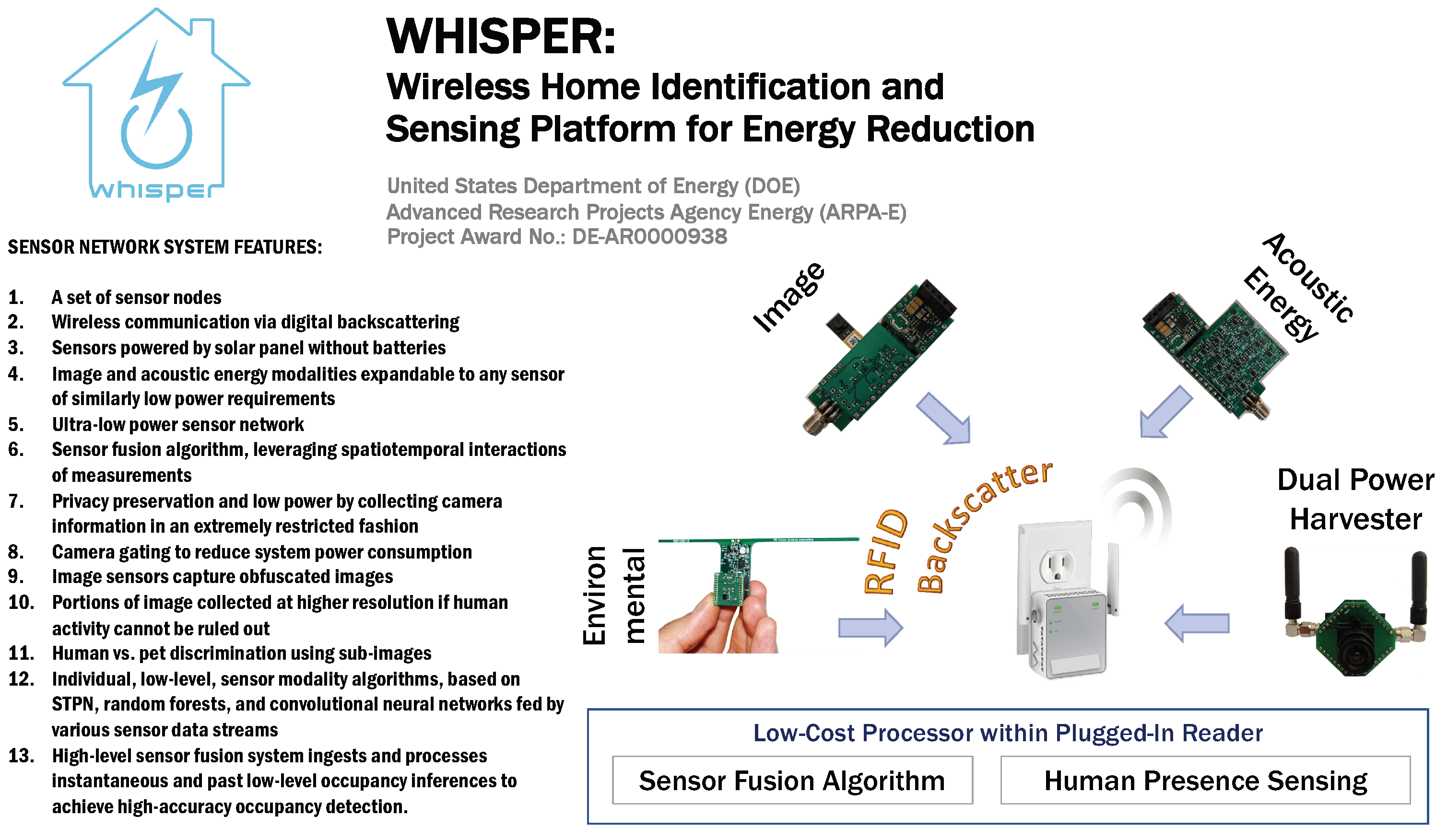
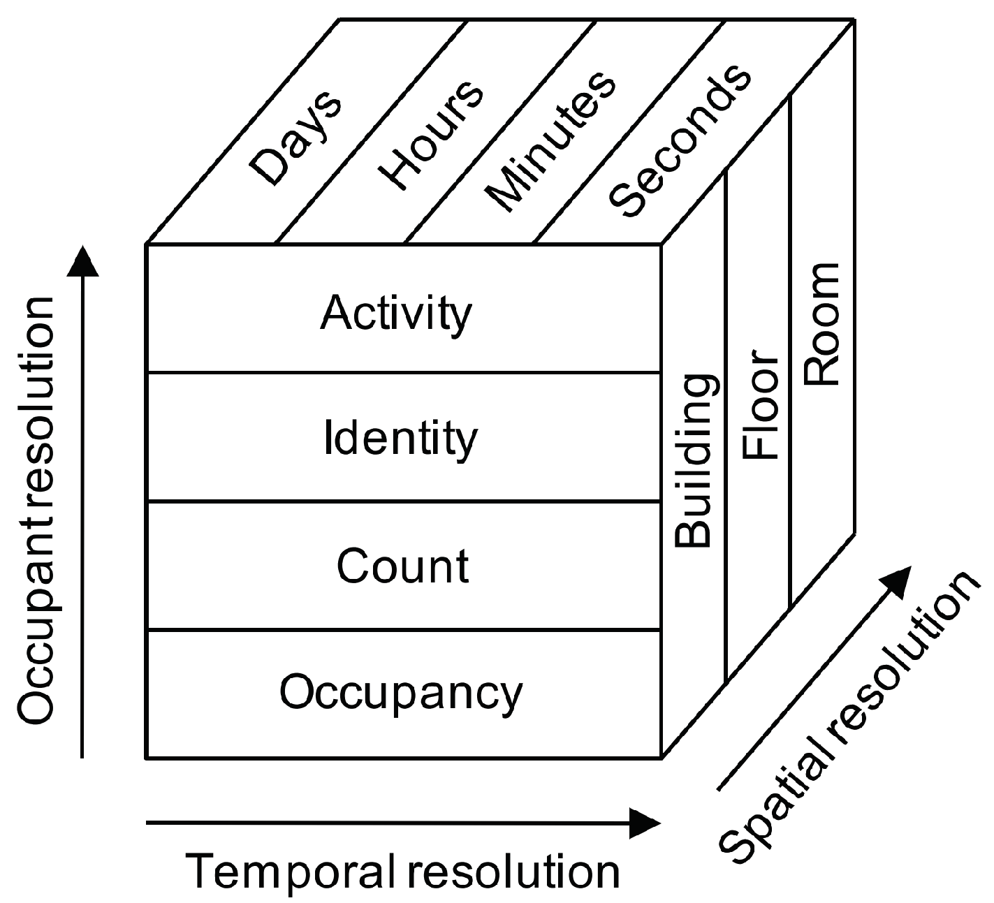

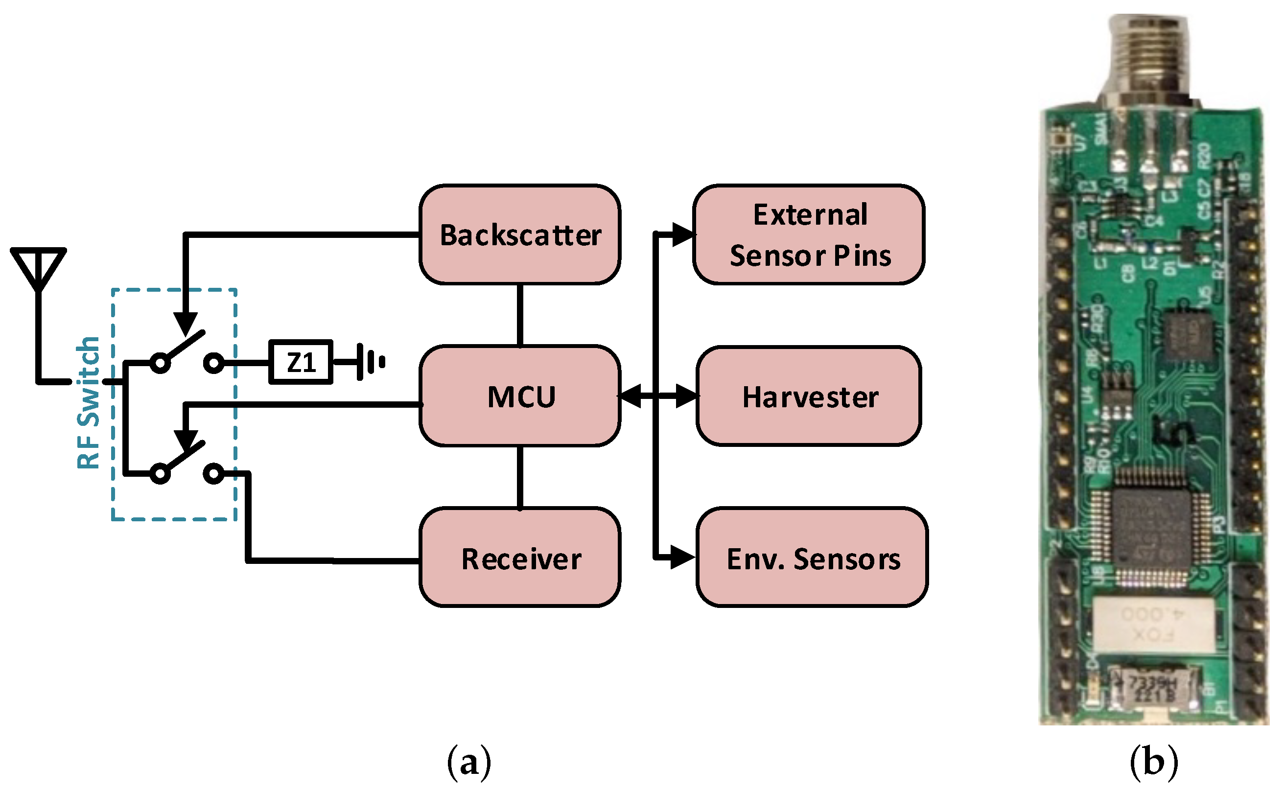

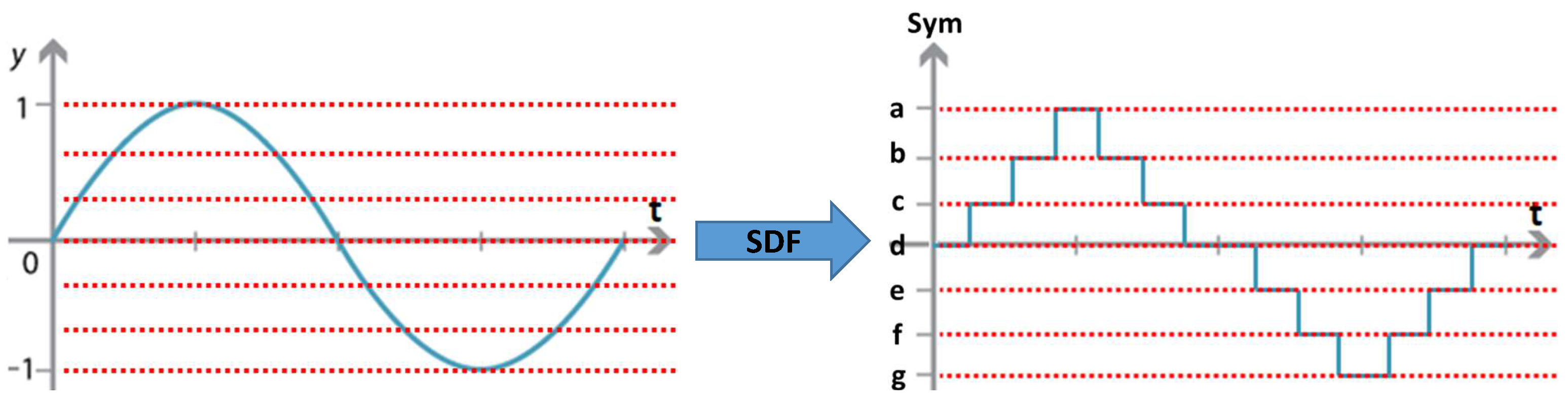

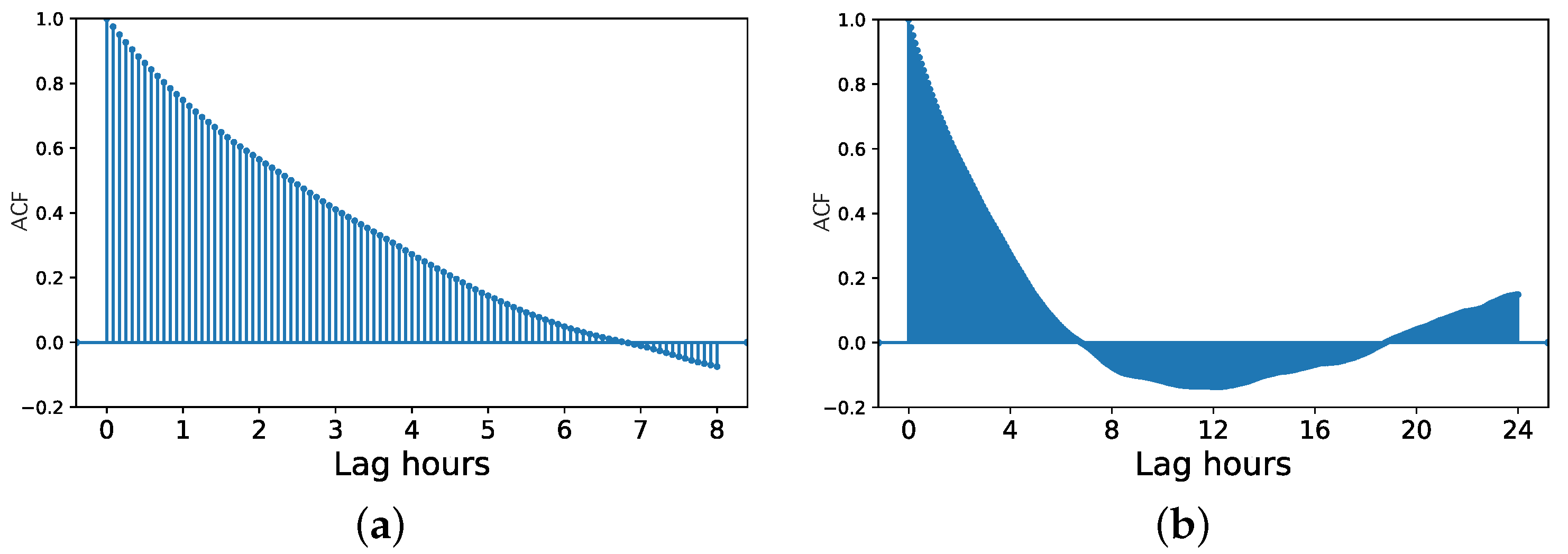
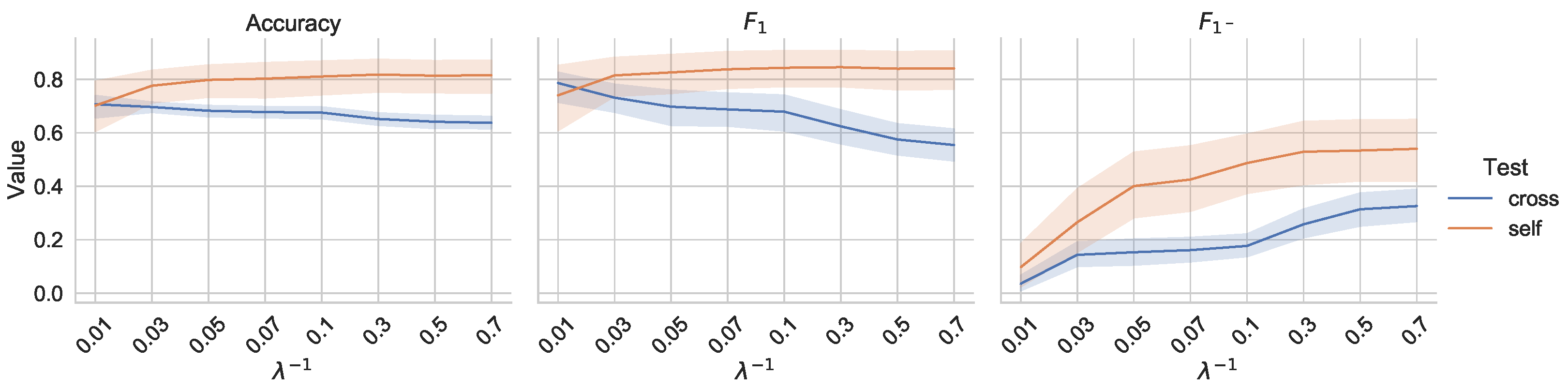

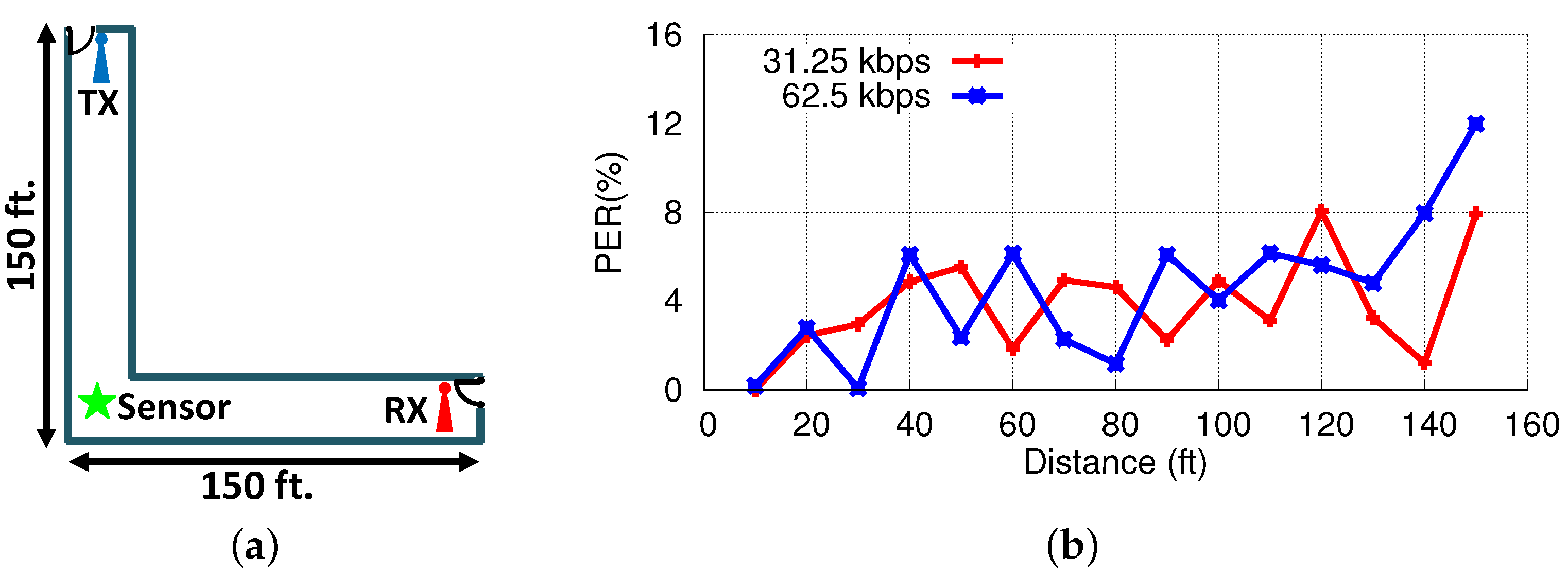
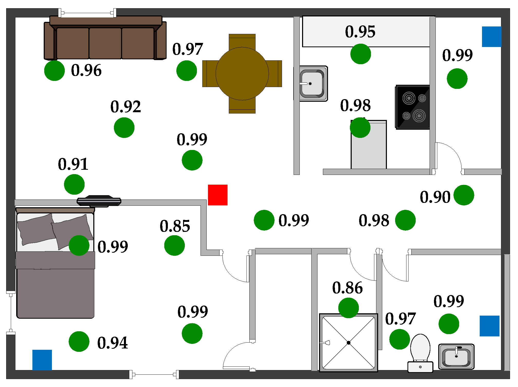
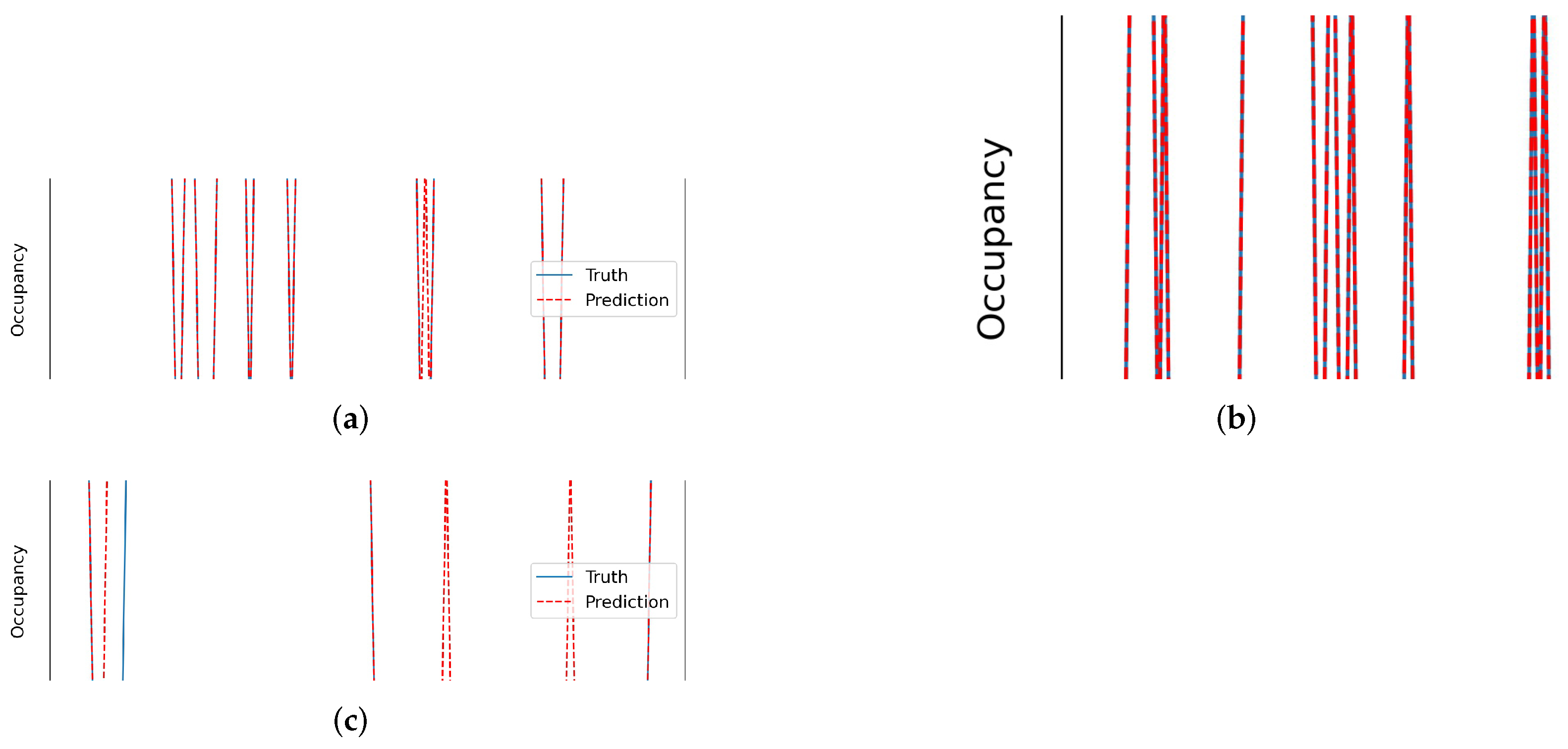
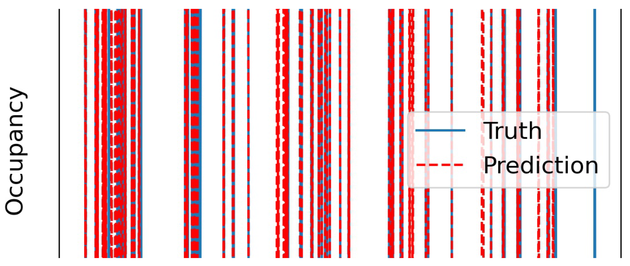
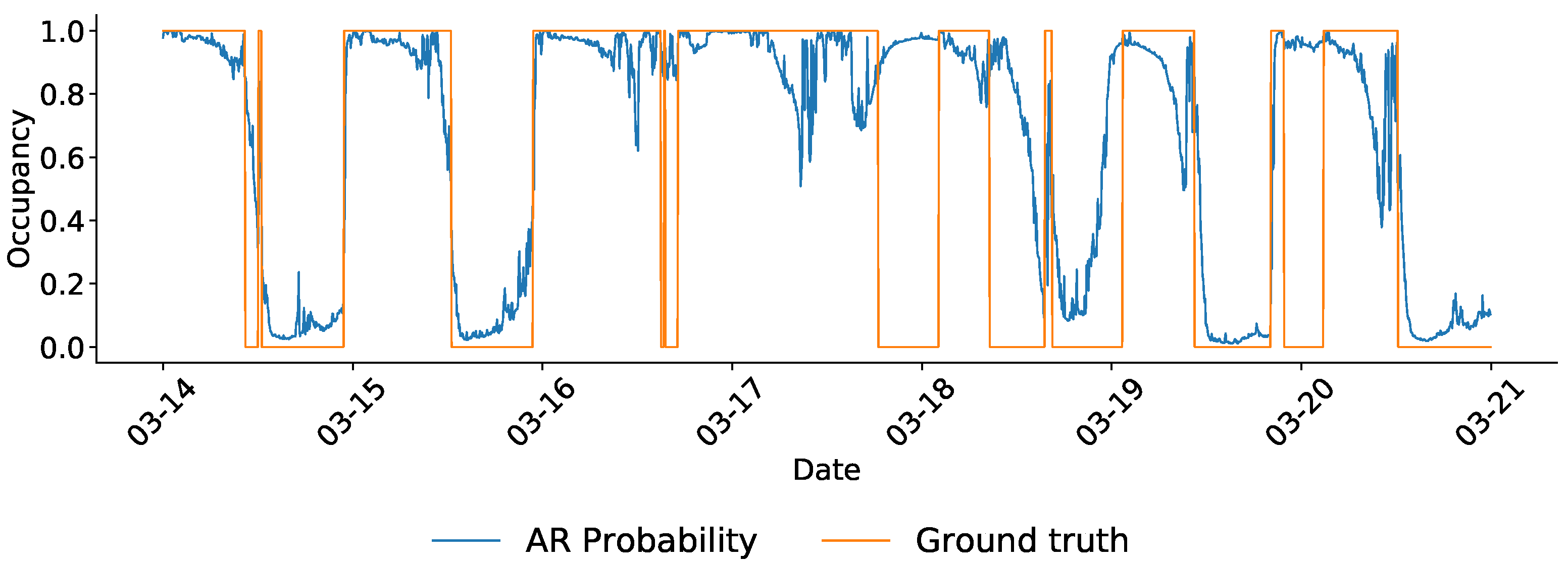
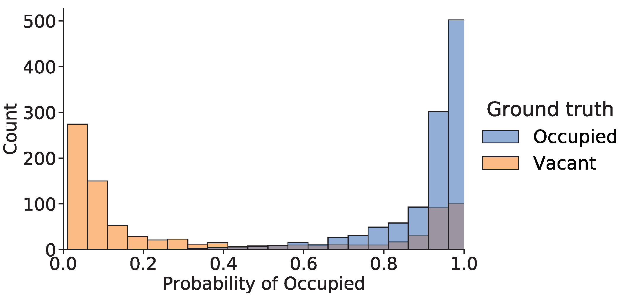
Publisher’s Note: MDPI stays neutral with regard to jurisdictional claims in published maps and institutional affiliations. |
© 2021 by the authors. Licensee MDPI, Basel, Switzerland. This article is an open access article distributed under the terms and conditions of the Creative Commons Attribution (CC BY) license (https://creativecommons.org/licenses/by/4.0/).