
Predictive Models for Aggregate Available Capacity Prediction in Vehicle-to-Grid Applications


Abstract
1. Introduction
- We integrate and standardize different data sources, combining readily accessible FCD data on mobility patterns with weather conditions and calendar information. This seamless integration enhances the accuracy and reliability of V2G applications, ensuring that our methods can be readily adopted and replicated and thereby facilitating broader application and validation within the V2G and energy grid research community.
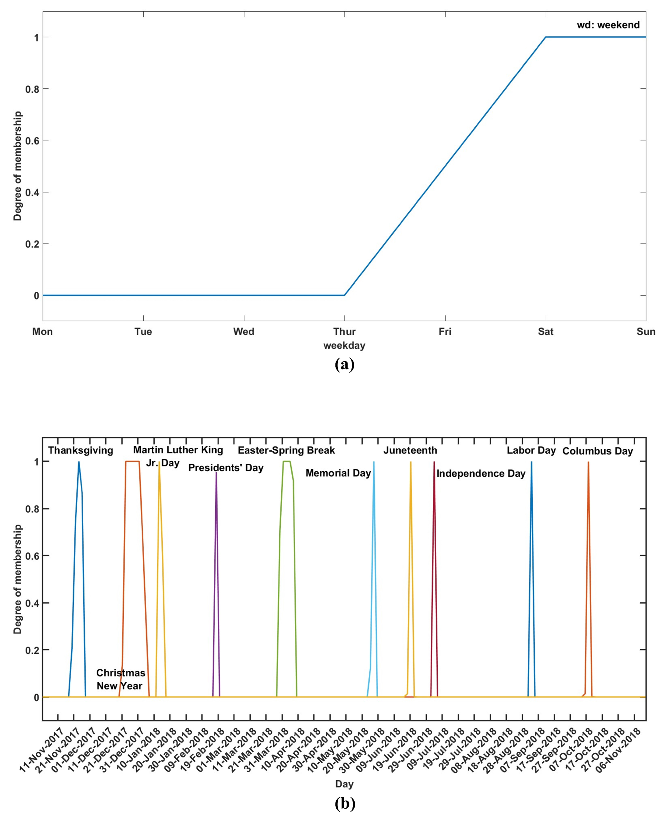
- We leverage fuzzy logic to derive a continuous and integrated holiday rate metric, a novel approach introduced as a proof of concept in [23]. This method synthesizes inputs from calendars, weekends, and national holidays, providing a continuous and accurate representation of holiday periods and allowing the model to learn driver habits from a one-year dataset.
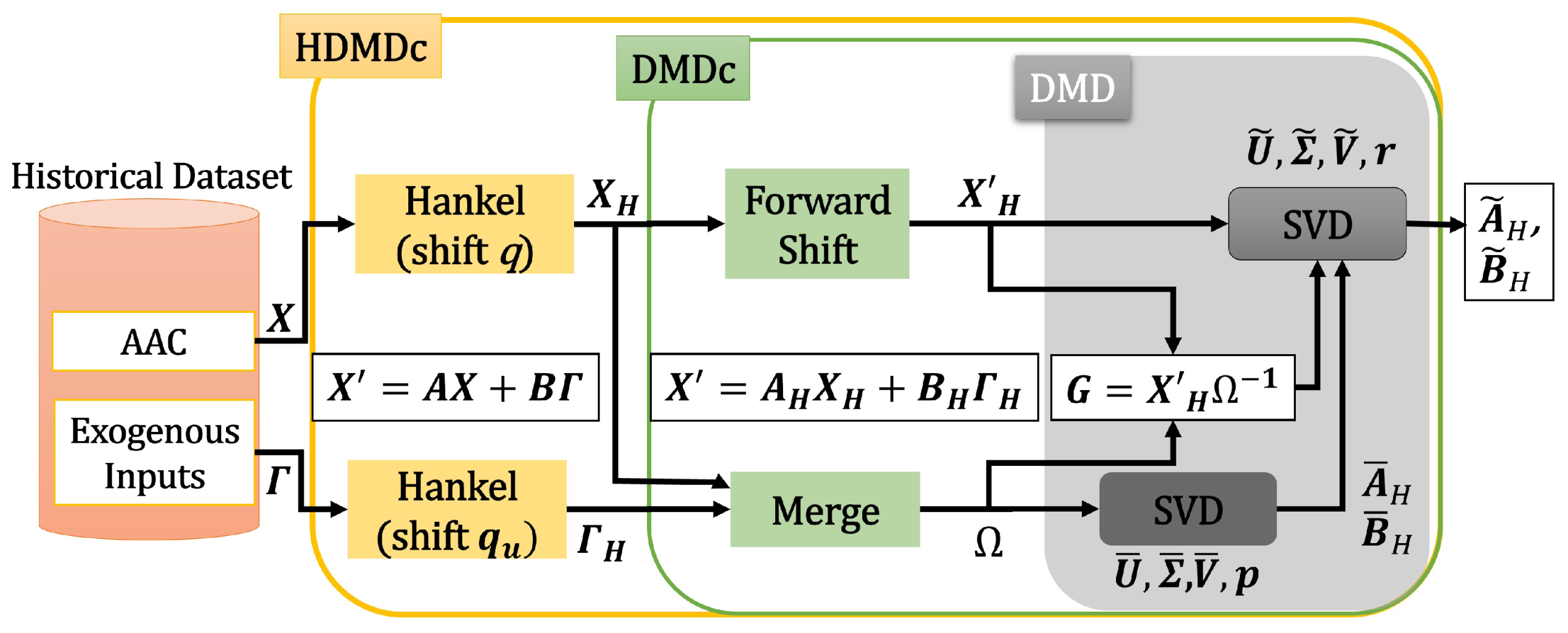
- We propose using HDMDc as a state-space representation method, contrasting with the well-established LSTM networks and other black-box models commonly used in time series forecasting, particularly in the V2G field. This offers a novel perspective with potential improvements in model performance, interpretability, and transferability.
2. Related Works

| Model | Prediction | Data | Exogenous Inputs | Model Class | Target |
|---|---|---|---|---|---|
| Persistence model, Generalized linear model, NN [32] | Half-hour-ahead | Hub | Calendar, Weekends | Deterministic, Data-driven Dynamic Linear, Dynamic Nonlinear Black-Box | AAC |
| NN, LSTM [23] | Half-hour-ahead | Generic FCD Data | Meteo, Fuzzy Weekend and Holiday rate | Dynamic Nonlinear Black-Box | AAC |
| MAML-CNN-LSTM-Attention Algorithm [33] | Hour-ahead | EVs limited fleet (Rental Car Fleet) | - | Dynamic Nonlinear Black-Box | AAC |
| K-Means clustering, LSTM using federated learning [35] | Hour-ahead | Hub | Calendar, Weekends | Dynamic Nonlinear Black-Box | Energy demand |
| Multilayer perceptron (MLP) [38] | Hour-ahead | Simulated EVs and Consumer preferences | Calendar, Meteo | Dynamic Nonlinear Black-Box | Load forecast for electricity price determination |
| LSTM [36] | Offline (day-ahead) Rolling (hour-ahead) | EVs fleet | - | Dynamic Nonlinear Black-Box | SEC |
| GBDT [37] | Offline (Day-ahead) Rolling (hour-ahead) | Generic FCD Data | - | Dynamic Nonlinear Black-Box | SEC |
| CNN-LSTM [27,28] | Day-ahead | EVs Limited fleet | None/Market event | Dynamic Nonlinear Black-Box | AAC |
| LSTM, NAR [34] | Day-ahead | EVs Limited fleet | Market event simulation | Dynamic Nonlinear Black-Box | AAC |
| RF, SARIMA [39] | Day-ahead | Hub | Calendar | Dynamic Nonlinear Black-Box, Data-Driven Dynamic Linear | Occupancy and charging load for single EV |
| XGBoost [40] | Yearly | EVs limited fleet/Simulated Data | - | Dynamic Nonlinear Black-Box | FCR participation |
| Analytical: Vehicle contribution sum [41] | - | Generic FCD Data (Mobile Phone GPS) | - | Static Deterministic | Daily Aggregated V2G ES and PD |
| Analytical [42] | - | EVs limited fleet (Shared Mobility on Demand) | Energy price | Static Deterministic | Driver preference for V2G or mobility |
| HDMDc—This study | Rolling 1 to 4 hour-ahead | Generic FCD Data | Meteo, Fuzzy Weekend and Holiday rate | Data-Driven Dynamic Linear State Space | AAC |
3. Methods: Theoretical Background
3.1. HDMDc
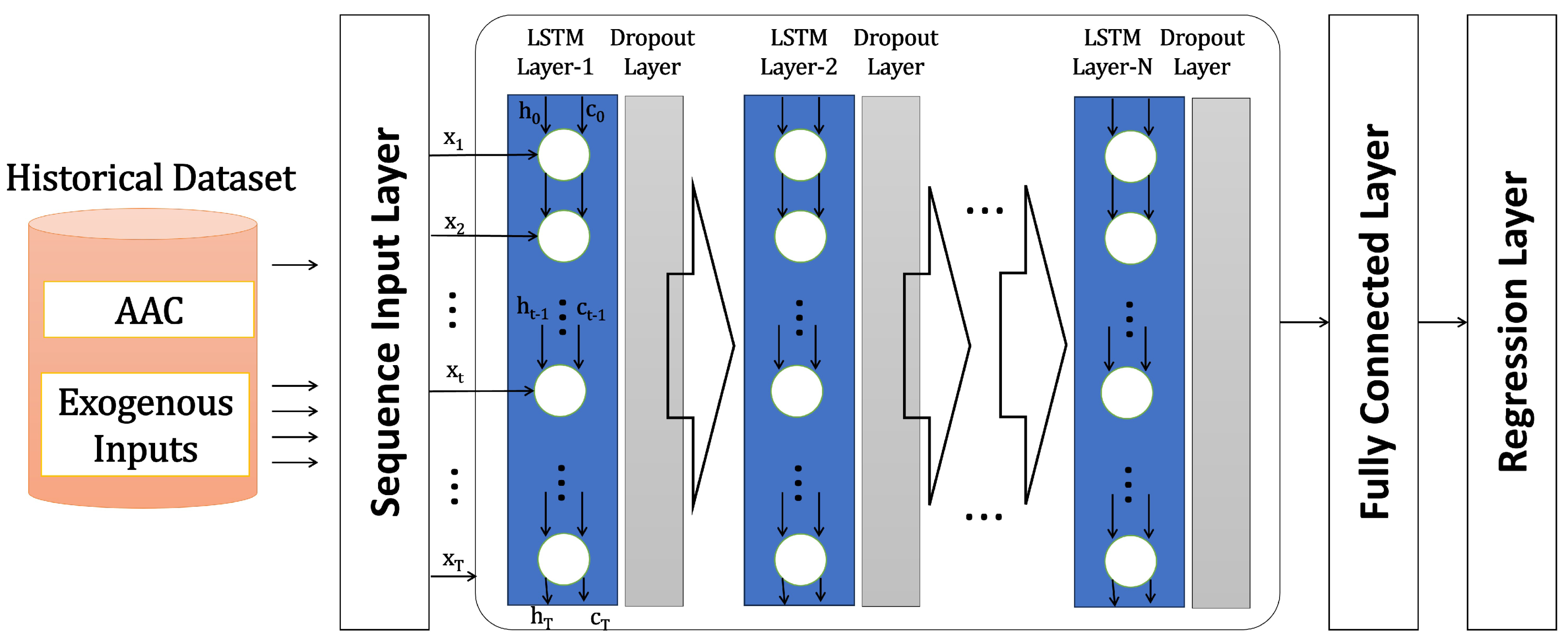
3.2. LSTM
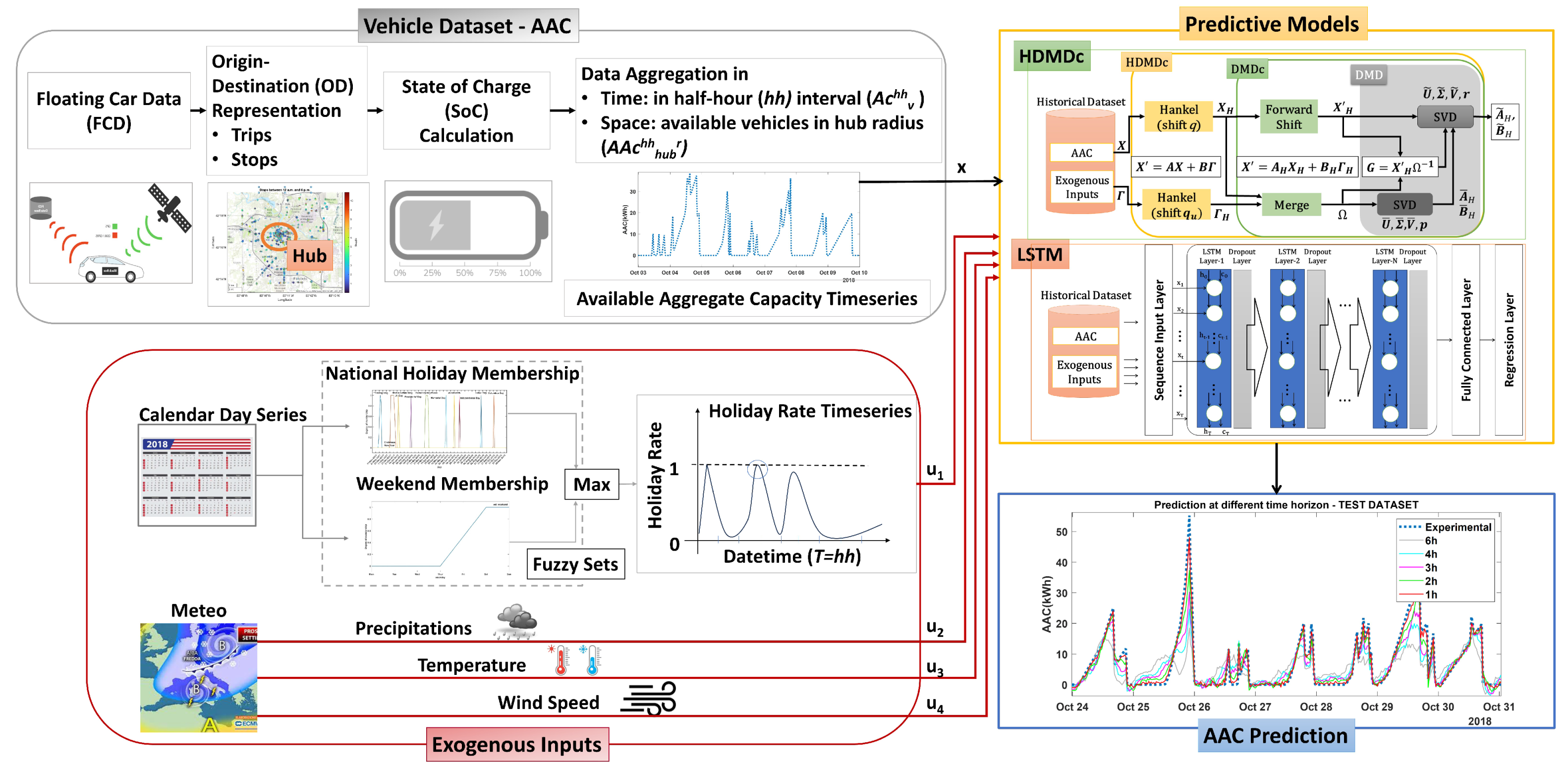
4. System Model
4.1. Data Collection and Pre-Processing
4.1.1. Vehicle Dataset
- Maximum battery charge at the start of the simulation:
- The minimum state of charge that must be maintained is set as a fixed value to cover the remaining part of the travel chain:
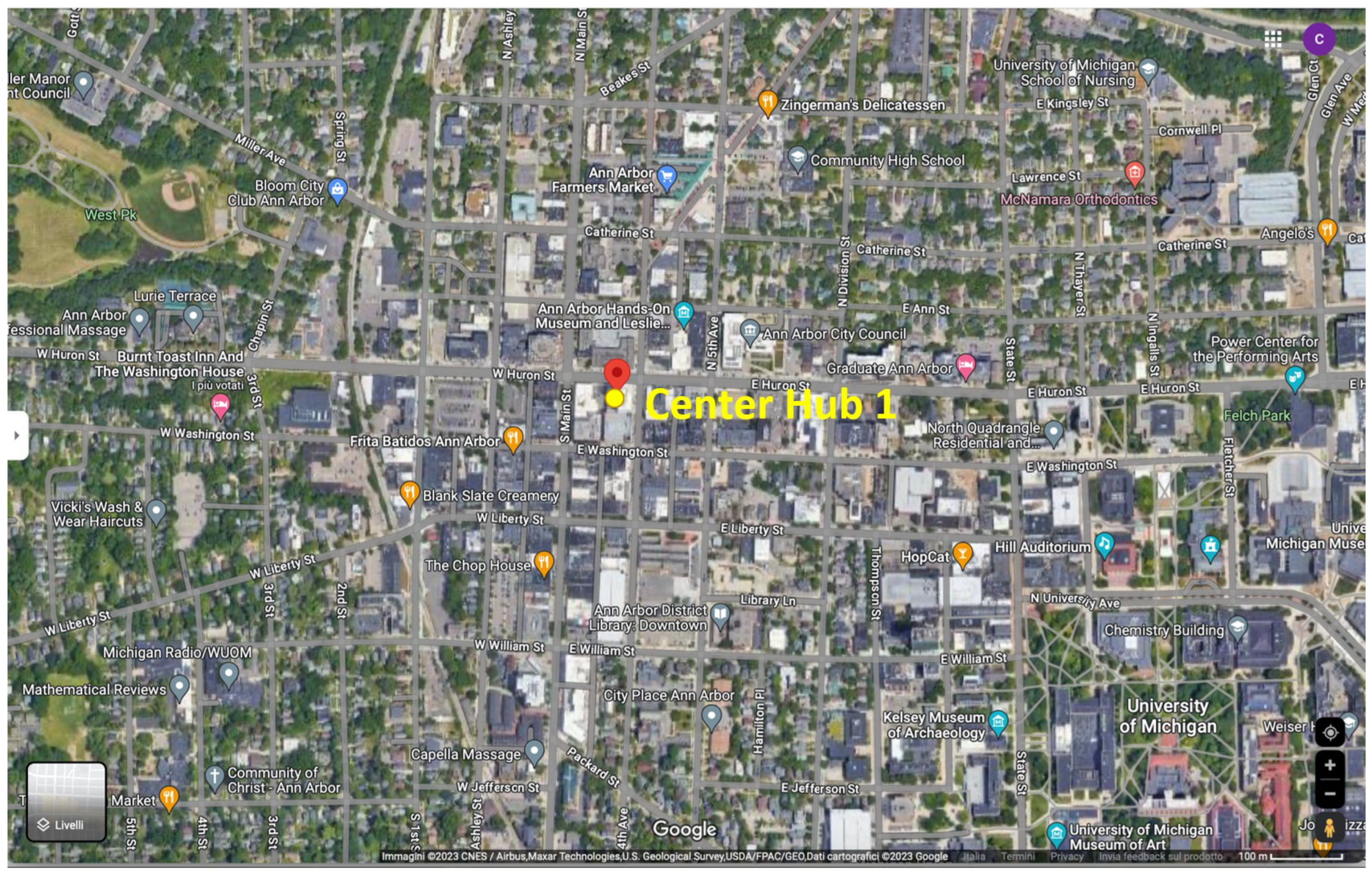
- The vehicles are considered available to supply energy to the grid when they are close to the hub and
- The energy consumption per kilometer traveled by a vehicle: km/kWh
- Rapid charging hour rating of a vehicle, typically using DC power, in the period from 7 a.m. to 7 p.m.: 50 kW
- Slow-charging hour rating of a vehicle in the time interval from 7 p.m. to 7 a.m.: 6 kW
- Efficiency of the charging process taking losses into account:
- Power rating of the export to the grid: 50 kW
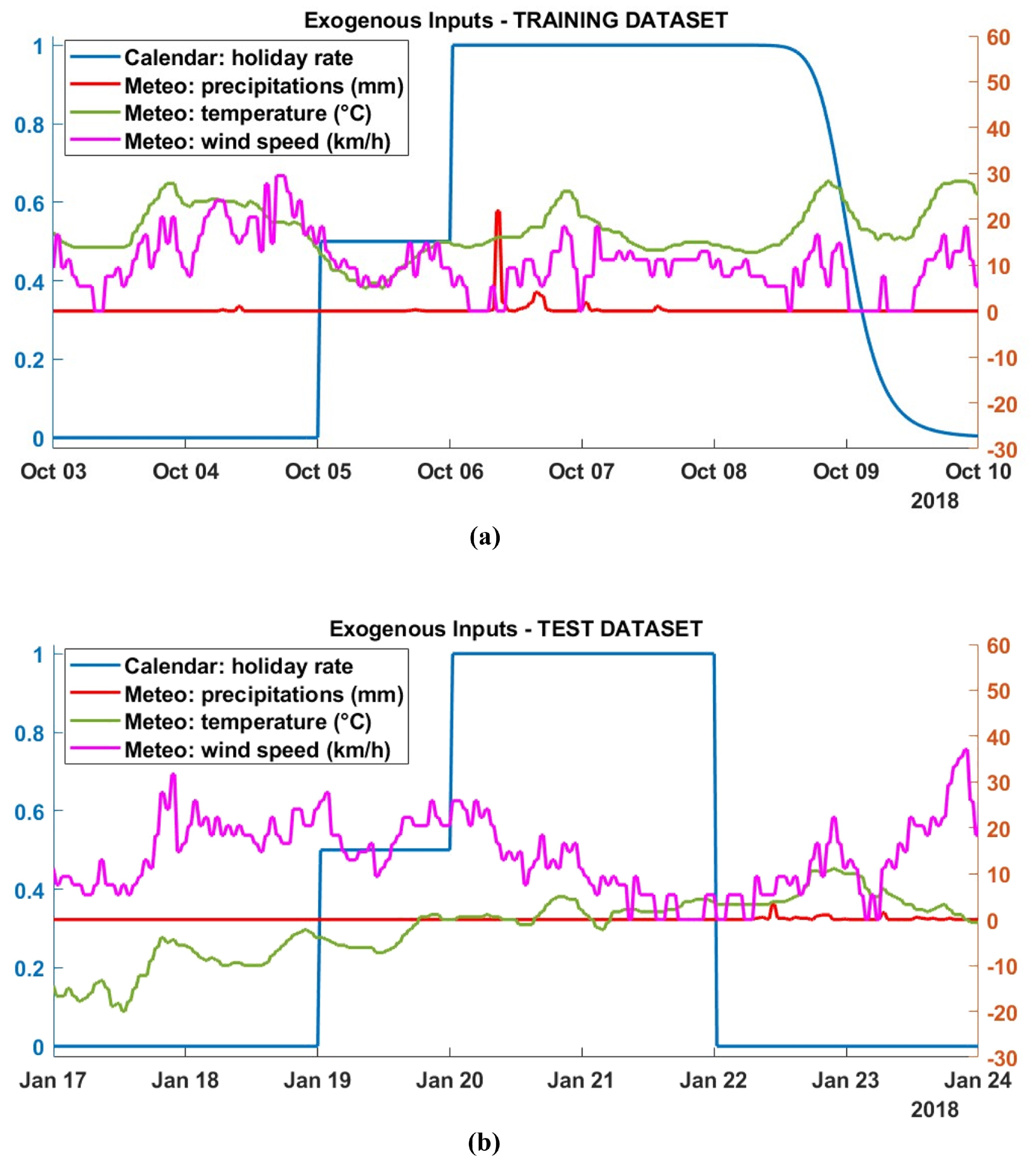
4.1.2. Meteorological Dataset
4.1.3. National Holidays Dataset
4.2. Model Prediction Analysis
4.2.1. HDMDc
4.2.2. LSTM
5. Results and Discussion
5.1. Learning Procedure
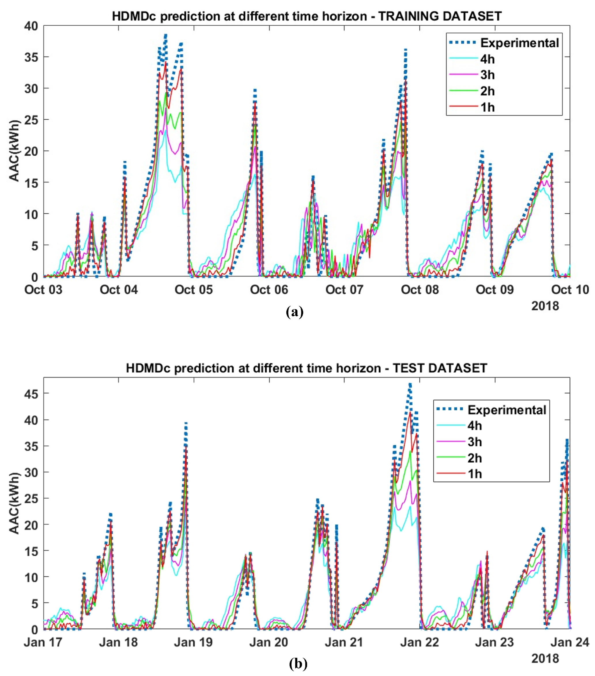
5.2. HDMDc
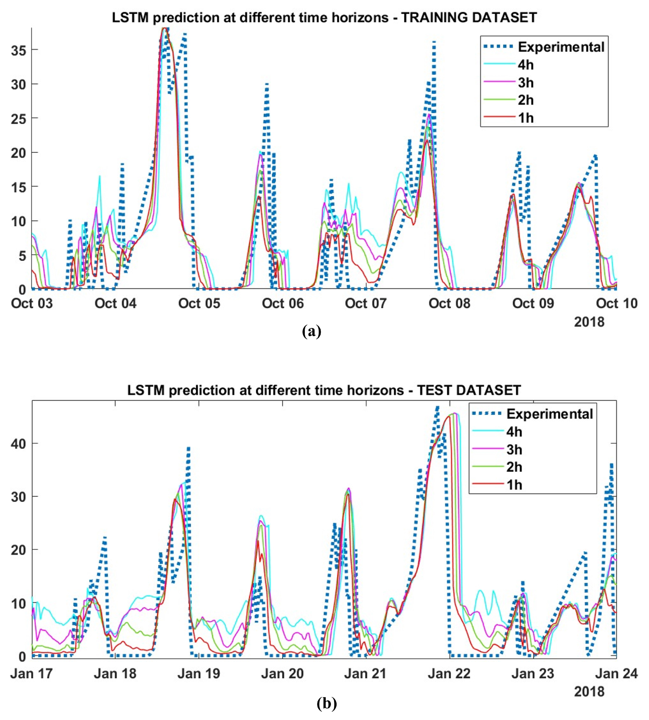
5.3. LSTM
- the LSTM depth between 1 and 3
- the number of hidden units between 50 and 350
- the dropout probability between and
- initial learn rate between and
6. Conclusions
Author Contributions
Funding
Data Availability Statement
Conflicts of Interest
Abbreviations
| V2G | Vehicle-to-Grid |
| SG | Smart Grids |
| AAC | Available Aggregate Capacity |
| IoT | Internet of Things |
| FCD | Floating Car Data |
| OD | Origin-Destination |
| ICE | Internal Combustion Engine |
| HEV | Hybrid Electric Vehicle |
| PHEV | Plug-in Hybrid Electric Vehicle |
| EV | Electric vehicle |
| SoC | State of Charge |
| hh | Half Hour |
| HDMDc | Hankel Dynamic Mode Decomposition with Control |
| LSTM | Long Short-Term Memory |
References
- International Energy Agency. By 2030 EVs Represent More Than 60% of Vehicles Sold Globally, and Require an Adequate Surge in Chargers Installed in Buildings. In Proceedings of the IEA, Paris, 2022. Available online: https://www.iea.org/reports/by-2030-evs-represent-more-than-60-of-vehicles-sold-globally-and-require-an-adequate-surge-in-chargers-installed-in-buildings (accessed on 20 June 2024).
- International Energy Agency. Net Zero by 2050. A Roadmap for the Global Energy Sector. In Proceedings of the IEA, Paris, 2021. Available online: https://www.iea.org/reports/net-zero-by-2050 (accessed on 20 June 2024).
- Kamble, S.G.; Vadirajacharya, K.; Patil, U.V. Decision Making in Power Distribution System Reconfiguration by Blended Biased and Unbiased Weightage Method. J. Sens. Actuator Netw. 2019, 8, 20. [Google Scholar] [CrossRef]
- Ding, B.; Li, Z.; Li, Z.; Xue, Y.; Chang, X.; Su, J.; Jin, X.; Sun, H. A CCP-based distributed cooperative operation strategy for multi-agent energy systems integrated with wind, solar, and buildings. Appl. Energy 2024, 365, 123275. [Google Scholar] [CrossRef]
- Zhang, R.; Chen, Y.; Li, Z.; Jiang, T.; Li, X. Two-stage robust operation of electricity-gas-heat integrated multi-energy microgrids considering heterogeneous uncertainties. Appl. Energy 2024, 371, 123690. [Google Scholar] [CrossRef]
- Zhang, H.; Li, Z.; Xue, Y.; Chang, X.; Su, J.; Wang, P.; Guo, Q.; Sun, H. A Stochastic Bi-level Optimal Allocation Approach of Intelligent Buildings Considering Energy Storage Sharing Services. IEEE Trans. Consum. Electron. 2024, 1. [Google Scholar] [CrossRef]
- Naja, R.; Soni, A.; Carletti, C. Electric Vehicles Energy Management for Vehicle-to-Grid 6G-Based Smart Grid Networks. J. Sens. Actuator Netw. 2023, 12, 79. [Google Scholar] [CrossRef]
- Mojumder, M.R.H.; Ahmed Antara, F.; Hasanuzzaman, M.; Alamri, B.; Alsharef, M. Electric Vehicle-to-Grid (V2G) Technologies: Impact on the Power Grid and Battery. Sustainability 2022, 14, 13856. [Google Scholar] [CrossRef]
- Bortotti, M.F.; Rigolin, P.; Udaeta, M.E.M.; Grimoni, J.A.B. Comprehensive Energy Analysis of Vehicle-to-Grid (V2G) Integration with the Power Grid: A Systemic Approach Incorporating Integrated Resource Planning Methodology. Appl. Sci. 2023, 13, 11119. [Google Scholar] [CrossRef]
- Lillebo, M.; Zaferanlouei, S.; Zecchino, A.; Farahmand, H. Impact of large-scale EV integration and fast chargers in a Norwegian LV grid. J. Eng. 2019, 2019, 5104–5108. [Google Scholar] [CrossRef]
- Deb, S.; Tammi, K.; Kalita, K.; Mahanta, P. Impact of Electric Vehicle Charging Station Load on Distribution Network. Energies 2018, 11, 178. [Google Scholar] [CrossRef]
- Grasel, B.; Baptista, J.; Tragner, M. The Impact of V2G Charging Stations (Active Power Electronics) to the Higher Frequency Grid Impedance. Sustain. Energy Grids Netw. 2024, 38, 101306. [Google Scholar] [CrossRef]
- Fachrizal, R.; Qian, K.; Lindberg, O.; Shepero, M.; Adam, R.; Widén, J.; Munkhammar, J. Urban-scale energy matching optimization with smart EV charging and V2G in a net-zero energy city powered by wind and solar energy. eTransportation 2024, 20, 100314. [Google Scholar] [CrossRef]
- Karmaker, A.K.; Prakash, K.; Siddique, M.N.I.; Hossain, M.A.; Pota, H. Electric vehicle hosting capacity analysis: Challenges and solutions. Renew. Sustain. Energy Rev. 2024, 189, 113916. [Google Scholar] [CrossRef]
- Paine, G. Understanding the True Value of V2G. An Analysis of the Customers and Value Streams for V2G in the UK, Cenex, 2019. Available online: https://www.cenex.co.uk/app/uploads/2019/10/True-Value-of-V2G-Report.pdf (accessed on 20 June 2024).
- Afentoulis, K.D.; Bampos, Z.N.; Vagropoulos, S.I.; Keranidis, S.D.; Biskas, P.N. Smart charging business model framework for electric vehicle aggregators. Appl. Energy 2022, 328, 120179. [Google Scholar] [CrossRef]
- Barbero, M.; Corchero, C.; Canals Casals, L.; Igualada, L.; Heredia, F.J. Critical evaluation of European balancing markets to enable the participation of Demand Aggregators. Appl. Energy 2020, 264, 114707. [Google Scholar] [CrossRef]
- Dixon, J.; Bukhsh, W.; Bell, K.; Brand, C. Vehicle to grid: Driver plug-in patterns, their impact on the cost and carbon of charging, and implications for system flexibility. eTransportation 2022, 13, 100180. [Google Scholar] [CrossRef]
- Comi, A.; Rossolov, A.; Polimeni, A.; Nuzzolo, A. Private Car O-D Flow Estimation Based on Automated Vehicle Monitoring Data: Theoretical Issues and Empirical Evidence. Information 2021, 12, 493. [Google Scholar] [CrossRef]
- Li, M.; Wang, Y.; Peng, P.; Chen, Z. Toward Efficient Smart Management: A Review of Modeling and Optimization Approaches in Electric Vehicle-Transportation Network-Grid Integration. Green Energy Intell. Transp. 2024, 100181. [Google Scholar] [CrossRef]
- Bakhshi, V.; Aghabayk, K.; Parishad, N.; Shiwakoti, N. Evaluating Rainy Weather Effects on Driving Behaviour Dimensions of Driving Behaviour Questionnaire. J. Adv. Transp. 2022, 2022, 1–10. [Google Scholar] [CrossRef]
- Gim, T.H.T. SEM application to the household travel survey on weekends versus weekdays: The case of Seoul, South Korea. Eur. Transp. Res. Rev. 2018, 10, 11. [Google Scholar] [CrossRef]
- Napoli, G.; Patanè, L.; Sapuppo, F.; Xibilia, M.G. A Comprehensive Data Analysis for Aggregate Capacity Forecasting in Vehicle-to-Grid Applications. In Proceedings of the 8th International Conference on Control, Automation and Diagnosis (ICCAD’24), Paris, France, 15–17 May 2024. [Google Scholar]
- Proctor, J.L.; Brunton, S.L.; Kutz, J.N. Dynamic Mode Decomposition with Control. SIAM J. Appl. Dyn. Syst. 2016, 15, 142–161. [Google Scholar] [CrossRef]
- Swathi Prathaa, P.; Rambabu, S.; Ramachandran, A.; Krishna, U.V.; Menon, V.K.; Lakshmikumar, S. Deep Learning and Dynamic Mode Decomposition for Inflation and Interest Rate Forecasting. In Proceedings of the 2022 13th International Conference on Computing Communication and Networking Technologies (ICCCNT), Kharagpur, India, 3–5 October 2022; pp. 1–7. [Google Scholar] [CrossRef]
- Curreri, F.; Patanè, L.; Xibilia, M.G. RNN- and LSTM-Based Soft Sensors Transferability for an Industrial Process. Sensors 2021, 21, 823. [Google Scholar] [CrossRef]
- Shipman, R.; Roberts, R.; Waldron, J.; Rimmer, C.; Rodrigues, L.; Gillott, M. Online Machine Learning of Available Capacity for Vehicle-to-Grid Services during the Coronavirus Pandemic. Energies 2021, 14, 7176. [Google Scholar] [CrossRef]
- Shipman, R.; Roberts, R.; Waldron, J.; Naylor, S.; Pinchin, J.; Rodrigues, L.; Gillott, M. We got the power: Predicting available capacity for vehicle-to-grid services using a deep recurrent neural network. Energy 2021, 221, 119813. [Google Scholar] [CrossRef]
- Mustavee, S.; Agarwal, S.; Enyioha, C.; Das, S. A linear dynamical perspective on epidemiology: Interplay between early COVID-19 outbreak and human mobility. Nonlinear Dyn. 2022, 109, 1233–1252. [Google Scholar] [CrossRef] [PubMed]
- Shabab, K.R.; Mustavee, S.; Agarwal, S.; Zaki, M.H.; Das, S. Exploring DMD-type Algorithms for Modeling Signalised Intersections. arXiv 2021, arXiv:2107.06369v1. [Google Scholar]
- Das, S.; Mustavee, S.; Agarwal, S.; Hasan, S. Koopman-Theoretic Modeling of Quasiperiodically Driven Systems: Example of Signalized Traffic Corridor. IEEE Trans. Syst. Man Cybern. Syst. 2023, 53, 4466–4476. [Google Scholar] [CrossRef]
- Graham, J.; Teng, F. Vehicle-to-Grid Plug-in Forecasting for Participation in Ancillary Services Markets. In Proceedings of the 2023 IEEE Belgrade PowerTech, Belgrade, Serbia, 25–29 June 2023. [Google Scholar] [CrossRef]
- Xu, M.; Ren, H.; Chen, P.; Xin, G. On the V2G capacity of shared electric vehicles and its forecasting through MAML-CNN-LSTM-Attention algorithm. IET Gener. Transm. Distrib. 2024, 18, 1158–1171. [Google Scholar] [CrossRef]
- Nogay, H.S. Estimating the aggregated available capacity for vehicle to grid services using deep learning and Nonlinear Autoregressive Neural Network. Sustain. Energy Grids Netw. 2022, 29, 100590. [Google Scholar] [CrossRef]
- Perry, D.; Wang, N.; Ho, S.S. Energy Demand Prediction with Optimized Clustering-Based Federated Learning. In Proceedings of the 2021 IEEE Global Communications Conference (GLOBECOM), Madrid, Spain, 7–11 December 2021; pp. 1–6. [Google Scholar] [CrossRef]
- Li, S.; Gu, C.; Li, J.; Wang, H.; Yang, Q. Boosting Grid Efficiency and Resiliency by Releasing V2G Potentiality through a Novel Rolling Prediction-Decision Framework and Deep-LSTM Algorithm. IEEE Syst. J. 2021, 15, 2562–2570. [Google Scholar] [CrossRef]
- Mao, M.; Zhang, S.; Chang, L.; Hatziargyriou, N.D. Schedulable capacity forecasting for electric vehicles based on big data analysis. J. Mod. Power Syst. Clean Energy 2019, 7, 1651–1662. [Google Scholar] [CrossRef]
- Gautam, A.; Verma, A.K.; Srivastava, M. A Novel Algorithm for Scheduling of Electric Vehicle Using Adaptive Load Forecasting with Vehicle-to-Grid Integration. In Proceedings of the 2019 8th International Conference on Power Systems (ICPS), Jaipur, India, 20–22 December 2019; pp. 1–6. [Google Scholar] [CrossRef]
- Amara-Ouali, Y.; Goude, Y.; Hamrouche, B.; Bishara, M. A Benchmark of Electric Vehicle Load and Occupancy Models for Day-Ahead Forecasting on Open Charging Session Data. In Proceedings of the Thirteenth ACM International Conference on Future Energy Systems, New York, NY, USA, 11–16 May 2022; pp. 193–207. [Google Scholar] [CrossRef]
- Jahromi, S.N.; Abdollahi, A.; Heydarian-Forushani, E.; Shafiee, M. A Comprehensive Framework for Predicting Electric Vehicle’s Participation in Ancillary Service Markets; IET Smart Grid: London, UK, 2024. [Google Scholar]
- Schläpfer, M.; Chew, H.J.; Yean, S.; Lee, B.S. Using Mobility Patterns for the Planning of Vehicle-to-Grid Infrastructures that Support Photovoltaics in Cities. arXiv 2021, arXiv:2112.15006. [Google Scholar]
- Zeng, T.; Moura, S.; Zhou, Z. Joint Mobility and Vehicle-to-Grid Coordination in Rebalancing Shared Mobility-on-Demand Systems. IFAC PapersOnLine 2023, 56, 6642–6647. [Google Scholar] [CrossRef]
- Patanè, L.; Sapuppo, F.; Xibilia, M.G. Soft Sensors for Industrial Processes Using Multi-Step-Ahead Hankel Dynamic Mode Decomposition with Control. Electronics 2024, 13, 3047. [Google Scholar] [CrossRef]
- Hochreiter, S.; Schmidhuber, J. Long Short-Term Memory. Neural Comput. 1997, 9, 1735–1780. [Google Scholar] [CrossRef]
- Oh, G.; Leblanc, D.J.; Peng, H. Vehicle Energy Dataset (VED), a Large-Scale Dataset for Vehicle Energy Consumption Research. IEEE Trans. Intel. Trans. Sys. 2022, 23, 3302–3312. [Google Scholar] [CrossRef]
- Meteo Stat Phyton API. Available online: https://dev.meteostat.net/python/ (accessed on 1 October 2023).
- Ann Arbour School Breaks. Available online: https://annarborwithkids.com/articles/winter-spring-break-schedules-2022/ (accessed on 1 October 2023).
- Michigan ORS Non-Business Days. Available online: https://www.michigan.gov/psru/ors-non-business-days (accessed on 1 October 2023).


| Variable | Description | Units |
|---|---|---|
| Precipitation | Meteo exogenous inputs | mm |
| Temperature | Meteo exogenous inputs | °C |
| Wind Speed | Meteo exogenous inputs | km/h |
| Fuzzy holiday rate | Calendar exogenous inputs | |
| V2G Infrastructure | ||
| r | Hub area radius | km |
| State of Charge | % | |
| Available capacity for the single vehicle in half-h | kWh | |
| Area within r radius from the Hub | ||
| x = | Target variable for the area | kWh |
| Non-Business Day | Date |
|---|---|
| Weekends | Saturdays and Sundays |
| Thanksgiving Day | 23 November 2017 |
| Day after Thanksgiving | 24 November 2017 |
| Christmas (Eve and Day) | 24–25 December 2017 |
| New Year (Eve and Day) | 31 December 2017–1 January 2018 |
| Martin Luther King, Jr. Day | 15 January 2018 |
| President’s Day | 19 February 2018 |
| Memorial Day | 28 May 2018 |
| Juneteenth | 19 June 2018 |
| Independence Day | 4 July 2018 |
| Labor Day | 3 September 2018 |
| Columbus Day | 8 October 2018 |
| Veterans Day | 12 November 2018 |
| Train | Test | |||||
|---|---|---|---|---|---|---|
| Prediction | MAE | RMSE | MAE | RMSE | ||
| 1 h | 0.75 | 1.14 | 0.995 | 0.82 | 1.24 | 0.995 |
| 2 h | 1.78 | 2.65 | 0.971 | 1.89 | 2.86 | 0.972 |
| 3 h | 2.55 | 3.79 | 0.929 | 2.69 | 4.07 | 0.934 |
| 4 h | 3.27 | 4.82 | 0.859 | 3.47 | 5.20 | 0.869 |
| Train | Test | |||||
|---|---|---|---|---|---|---|
| Prediction | MAE | RMSE | R | MAE | RMSE | R |
| 1 h | 2.28 | 4.28 | 0.852 | 3.67 | 6.53 | 0.647 |
| 2 h | 3.21 | 4.93 | 0.80 | 4.63 | 7.29 | 0.54 |
| 3 h | 4.20 | 5.79 | 0.739 | 5.68 | 8.06 | 0.456 |
| 4 h | 5.10 | 6.65 | 0.677 | 6.57 | 8.78 | 0.385 |
Disclaimer/Publisher’s Note: The statements, opinions and data contained in all publications are solely those of the individual author(s) and contributor(s) and not of MDPI and/or the editor(s). MDPI and/or the editor(s) disclaim responsibility for any injury to people or property resulting from any ideas, methods, instructions or products referred to in the content. |
© 2024 by the authors. Licensee MDPI, Basel, Switzerland. This article is an open access article distributed under the terms and conditions of the Creative Commons Attribution (CC BY) license (https://creativecommons.org/licenses/by/4.0/).
Share and Cite
Patanè, L.; Sapuppo, F.; Napoli, G.; Xibilia, M.G. Predictive Models for Aggregate Available Capacity Prediction in Vehicle-to-Grid Applications. J. Sens. Actuator Netw. 2024, 13, 49. https://doi.org/10.3390/jsan13050049
Patanè L, Sapuppo F, Napoli G, Xibilia MG. Predictive Models for Aggregate Available Capacity Prediction in Vehicle-to-Grid Applications. Journal of Sensor and Actuator Networks. 2024; 13(5):49. https://doi.org/10.3390/jsan13050049
Chicago/Turabian StylePatanè, Luca, Francesca Sapuppo, Giuseppe Napoli, and Maria Gabriella Xibilia. 2024. "Predictive Models for Aggregate Available Capacity Prediction in Vehicle-to-Grid Applications" Journal of Sensor and Actuator Networks 13, no. 5: 49. https://doi.org/10.3390/jsan13050049
APA StylePatanè, L., Sapuppo, F., Napoli, G., & Xibilia, M. G. (2024). Predictive Models for Aggregate Available Capacity Prediction in Vehicle-to-Grid Applications. Journal of Sensor and Actuator Networks, 13(5), 49. https://doi.org/10.3390/jsan13050049