Article

Real-Time Damage Detection and Localization on Aerospace Structures Using Graph Neural Networks

Department of Mechanical and Aerospace Engineering (DIMA), Sapienza University of Rome, 00184 Rome, Italy
*
Author to whom correspondence should be addressed.
J. Sens. Actuator Netw. 2025, 14(5), 89; https://doi.org/10.3390/jsan14050089
Submission received: 22 July 2025 / Revised: 20 August 2025 / Accepted: 27 August 2025 / Published: 29 August 2025
(This article belongs to the Special Issue Fault Diagnosis in the Internet of Things Applications)

Abstract

This work presents a novel Graph Neural Network (GNN) based framework for structural damage detection and localization in composite aerospace structures. The sensor network is modeled as a graph whose nodes correspond to the strain measurement points placed on the system, while the edges capture spatial and structural relationships among sensors. Strain mode shapes, extracted via Automated Operational Modal Analysis (AOMA), are used as input features for the GNN. Two architectures are developed: one for binary damage detection and another for damage localization, the latter outputting a spatial probability distribution of damage over the structure. Both networks are trained and validated on synthetic datasets generated from high-fidelity finite element transient simulations performed on a composite wing equipped with 40 strain sensors. The obtained results show strong effectiveness in both detection and localization tasks, thus highlighting the potential of leveraging GNNs for topology-aware Structural Health Monitoring applications. In particular, the proposed framework achieves an AUC of 0.97 for damage detection and a mean localization error of approximately 3% of the wingspan on the synthetic dataset. The performance of the GNN is also compared with a fully connected and a convolutional neural network, demonstrating significant improvements in the localization accuracy.

1. Introduction

A primary concern in the design of aircraft structures is their vulnerability to damages induced by mechanical loads [1]. Within the civil aviation industry, maintenance is typically performed at scheduled intervals in order to ensure safety and reliability. However, this approach is expensive, with inspection and maintenance accounting for over 27% of an aircraft total lifecycle cost [2]. Therefore, current research is focusing on developing proactive strategies that rely on real-time monitoring of the system, optimizing maintenance practices based on the actual condition rather than on predefined schedules. Structural Health Monitoring (SHM) systems enable this scheme by processing real-time data coming from sensors installed on structure [3]. According to Rytter [4], the information obtained from SHM systems can be classified according to four distinct levels: the detection level identifies whether damage is present or not; the localization level determines the exact location of the affected area; the assessment level evaluates the severity and extent of the damage; and the prediction level estimates the remaining useful life of the structural component.
In recent years, significant efforts have been devoted to uncovering the latent relationships between measured signals from installed sensors and the corresponding damage states [5]. Some of the most promising tools to learn such relations are artificial intelligence methods, particularly Neural Networks (NNs). NNs can be trained using input data obtained through various SHM techniques, such as Electromechanical Impedance [6], Acoustic Emission [7], or Lamb waves [8], to identify and classify structural damage. Among the possible approaches, vibration-based methods [9] are based on the idea that a damage induces changes in the physical properties of the system (such as mass, damping, and stiffness), which in turn, affect its modal properties (natural frequencies, modal damping, and mode shapes) [10]: these modal features can be used as informative inputs for NNs. However, NNs typically require large volumes of training data. While experimental data can be limited, numerical simulations via finite element (FE) models offer a viable alternative for generating diverse damage scenarios, provided the model is accurate [11]. Nonetheless, it is important to note that simulated data differ from real measurements due to noise and modeling uncertainties and thus, an accurate tuning is necessary for the numerical model. Recent works have also explored out-of-distribution data augmentation to address the scarcity of damaged samples as performed by Chen et al. [12,13] who applied this strategy for fault detection in rotating machinery.
Several studies have explored the use of vibration-based features as input to fully connected neural networks for structural damage detection. As an example, Sahin and Shenoi [14] used both global dynamic features (frequency shifts) and local ones (mode shape curvatures) as inputs to a fully connected neural network, demonstrating its effectiveness on beam-like and laminated composite structures. Pagani et al. [15] employed the first natural frequencies and Modal Assurance Criterion (MAC) values as input features to estimate the location and severity of damage in different 1D numerical models of aeronautical components. Other works [16,17] have instead used Frequency Response Functions (FRFs) as inputs to neural networks to perform damage monitoring.
As the structural complexity increases, traditional fully connected NN may struggle with generalization and overfitting. To overcome these limitations, deep learning methods such as convolutional neural networks (CNNs) have been applied to SHM. CNNs, with their ability to extract spatial features through convolutional layers, have achieved notable results in damage detection [18]. For instance, Nguyen et al. [19] used contour images of mode shape curvature variations as input to train CNNs for damage detection in plate structures. In a recent application, Duran et al. [20] converted strain time histories into images to train a CNN for detecting damage in a bridge deck.
Most CNN applications assume that the data is arranged on regular Euclidean grids (e.g., 2D images or flat plates). However, real structures often have complex geometries, making this kind of representation non-trivial. On another hand, Graph Neural Networks (GNNs) can be used to generalize convolution to irregular, non-Euclidean domains [21] by modeling the sensor network as a graph. In this representation, nodes correspond to sensors and edges encode structural or spatial relationships [22]. GNNs aggregate information from neighboring nodes to iteratively refine node-level representations, enabling improved detection and localization performance. Recent studies have demonstrated the effectiveness of GNNs in SHM for some civil structures. Kim and Song [23] introduced a near-real-time seismic damage detection method based on GNNs. Son et al. [24] proposed a GNN to evaluate cross-sectional area reduction caused by fracture or corrosion experienced by bridges cables.
The aforementioned applications concern mainly cases involving reticular structures composed of one-dimensional elements. In the context of thin-walled and shell structures, recent works have explored alternative GNN-based formulations. For instance, Jiang et al. [25] developed a network to estimate the stress field of an offshore wind tower from a set of discrete measurements, while Pollet et al. [26] applied GNNs to predict the buckling load of thin shells. However, to the best of the authors’ knowledge, no studies have addressed damage detection and localization in aerospace structures using GNNs. These semi-monocoque structures exhibit an intricate mechanical behavior that poses additional challenges. Therefore, this study aims to develop a methodology capable of efficiently performing damage monitoring on typical aerospace structures based on Graph Neural Networks. The approach employs both strain mode shapes and topological information of the structure. Strain modes are used because they are more sensitive to local stiffness changes induced by damages than displacement modes [27]. Furthermore, working with modal data rather than raw time histories reduces the dimensionality of the input, allowing for a more compact GNN architecture and shorter training time, while maintaing a high-efficiency. In this work, two GNNs are developed: the first performs damage detection (i.e, a binary classification problem), while the second focuses on damage localization by estimating a spatial probability distribution over the sensor network. The proposed methodology is validated on a numerical model of a composite glider wing, where synthetic datasets are generated through FE simulations and combined with Automated Operational Modal Analysis applied on the strain time histories to estimate the modal properties. Indeed, AOMA techniques can be employed to estimate natural frequencies, damping ratios, and mode shapes under operational conditions, as they rely solely on output data acquired from sensors. The results of the two proposed GNNs demonstrate high performance in both damage detection and localization tasks. Furthermore, the performance of this framework is compared with that of a standard fully connected neural network and a convolutional network, showing significantly higher accuracy in both cases. These findings highlight the potential of geometry-based neural networks for Structural Health Monitoring of aerospace structures.

2. Theoretical Background

2.1. Automated Operational Modal Analysis

Operational Modal Analysis techniques allow the evaluation of the dynamic behavior of a structure under its actual boundary conditions and excitation levels, using vibration responses only. Several techniques have been developed, both in frequency and in the time domain, under the main common assumption that the excitation has to be stochastic with the same spectral characteristics as the white noise. Within the aeronautical field, Peeters et al. [28] demonstrated the effectiveness of natural turbulence excitation for in-flight modal analysis of a large aircraft, showing that it can yield similar modal parameters to those obtained with standard sine sweep excitation.

2.1.1. Stochastic Subspace Identification

The Stochastic Subspace Identification method uses the state space formulation to evaluate the dynamic behavior of a N degrees of freedom system (model order) represented by [29]
x ˙ ( t ) = A x ( t ) + B f ( t ) y ( t ) = C x ( t )
where y ( t ) N o is a stochastic response of the system ( N o is the number of outputs), the state is x ( t ) 2 N , the system matrix is A 2 N × 2 N , and the output matrix is C N o × 2 N . The load matrix is B 2 N × N i , and f N i represents the system input ( N i is the number of inputs).
In a discrete formulation, the system response can be expressed by the data matrix Y N o × N t , with N t number of data point
Y = y 1 , y 2 , . . . . . , y N t
Considering a total time shift 2 k , it is possible to build a block Hankel matrix Y h 2 k N o × ( N t 2 k ) by shifting the data matrices:
Y h = Y ( 1 : N t 2 k ) Y ( 2 : N t 2 k + 1 ) Y ( 2 k : N t ) = Y h p Y h f
in which the upper half part, Y h p k N o × ( N t 2 k ) , is referred to as the “the past”, while the lower half part, Y h p k N o × ( N t 2 k ) , is called “the future”. The total data shift 2 k is the number of block rows of such Hankel matrix.
Starting on the hypothesis of stochastic response, it is possible to define the covariances between the output measures at different time lags by a projection of the “future” onto the “past”:
Y h f / Y h p = Y h f Y h p T Y h f Y h p T 1 Y h p
where the expression Y h f / Y h p is a shorthand for the oblique projection of the row space of the matrix Y h f on the row space of the matrix Y h p . The last Y h p matrix in Equation (4) defines the initial conditions, and the first four matrices in the product introduce the covariances between channels at different time lags. Each column of Equation (4) consists of free decays of the system given by the different initial conditions specified by Y h p .
The definition of the projection provides a direct relation with the observability matrix O k of the system:
Y h f / Y h p = O k X 0
in which X 0 contains the initial condition at time lag zero. By comparing Equations (4) and (5), it is possible to find the observability matrix, passing through a singular value decomposition of the projection:
Y h f / Y h p = U S V T
O k = U S 1 / 2
Starting from the observability matrix, O k , it is possible to evaluate the system matrix A considering the definition in Equation (8):
O k = C C A C A k 1
Thus, the C matrix can be extracted from the first N o lines of O k , and CA from the next ones. As a result, the estimation of the A matrix is obtained by a least square procedure.
By solving the eigen-problem of the system matrix, it is possible to estimate the n-th pole of the system λ n = ζ n ω n ± j ω n , n = 1 , 2 , , N , with ζ n and ω n being the natural damping ratio and the natural frequency, whereas the n-th mode shape ϕ n is estimated from the respective eigenvectors. This process is reiterated by incrementing the unknown system order from a minimum to a maximum order.
Based on the principle that the poles which describe the dynamic behavior of the system are not dependent on the model order, those poles that remain constant as the model order is increased are selected as the potential set of physical poles. To identify only the physical poles from the solutions obtained via SSI, a two-stage validation strategy is implemented [30]. The first stage applies the so-called hard validation criteria, which aim to discard poles that violate basic physical constraints. Specifically, poles are rejected if they exhibit negative natural frequencies, negative damping ratios, or unrealistically high damping values, typically above 20%.
Following this initial filtering stage, soft validation criteria are applied to assess the stability of the remaining poles across different model orders. The idea is to compare the modal properties, frequency, damping, and mode shape (in terms of Modal Assurance Criterion, MAC), between the model order i and i + 2 , and verify that their variations remain within a predefined tolerance. In this work, a threshold of 2% is used for frequency and damping and a threshold of 98% is used for MAC. These values are close to those typically adopted in the literature, with the damping threshold being slightly more stringent given the synthetic nature of the dataset. Specifically, the criteria adopted are
f n i f n i + 2 f n i ε f n
ζ n i ζ n i + 2 ζ n i ε ζ n
MAC ϕ i , ϕ i + 2 = ϕ i H · ϕ i + 2 2 ( ϕ i H · ϕ i ) · ( ϕ i + 2 H · ϕ i + 2 ) MAC thr
To support the interpretation of pole stability and the application of these criteria, the stabilization diagram (Figure 1) is a commonly adopted tool in both Experimental and Operational Modal Analysis. This hybrid diagram displays the frequencies on the horizontal axis while using two distinct vertical axes: the left axis shows the Power Spectral Density (PSD) level, and the right axis indicates the system order of the poles. In this way, the diagram provides a combined view of how poles evolve with increasing model order and how they align with the dominant spectral peaks. Physical poles, which meet the stability thresholds, appear as vertical alignments, while non-physical or spurious poles tend to vary significantly with model order. The stabilization diagram is particularly useful to identify persistent modal parameters and guide the final selection of stable poles for further analysis. For each group of stable poles, a single representative is selected to represent a mode, typically based on the user’s expertise [31].

2.1.2. Automatic Selection of Poles

Traditionally, the identification of system poles from a stabilization diagram is performed manually by test engineers: this process is subjective and may introduce inconsistencies. The core idea behind the stabilization diagram is to track poles that remain stable in terms of modal properties as the model order increases. Because of this, clustering algorithms can be considered a valid option to automatically group poles with similar dynamic characteristics [32].
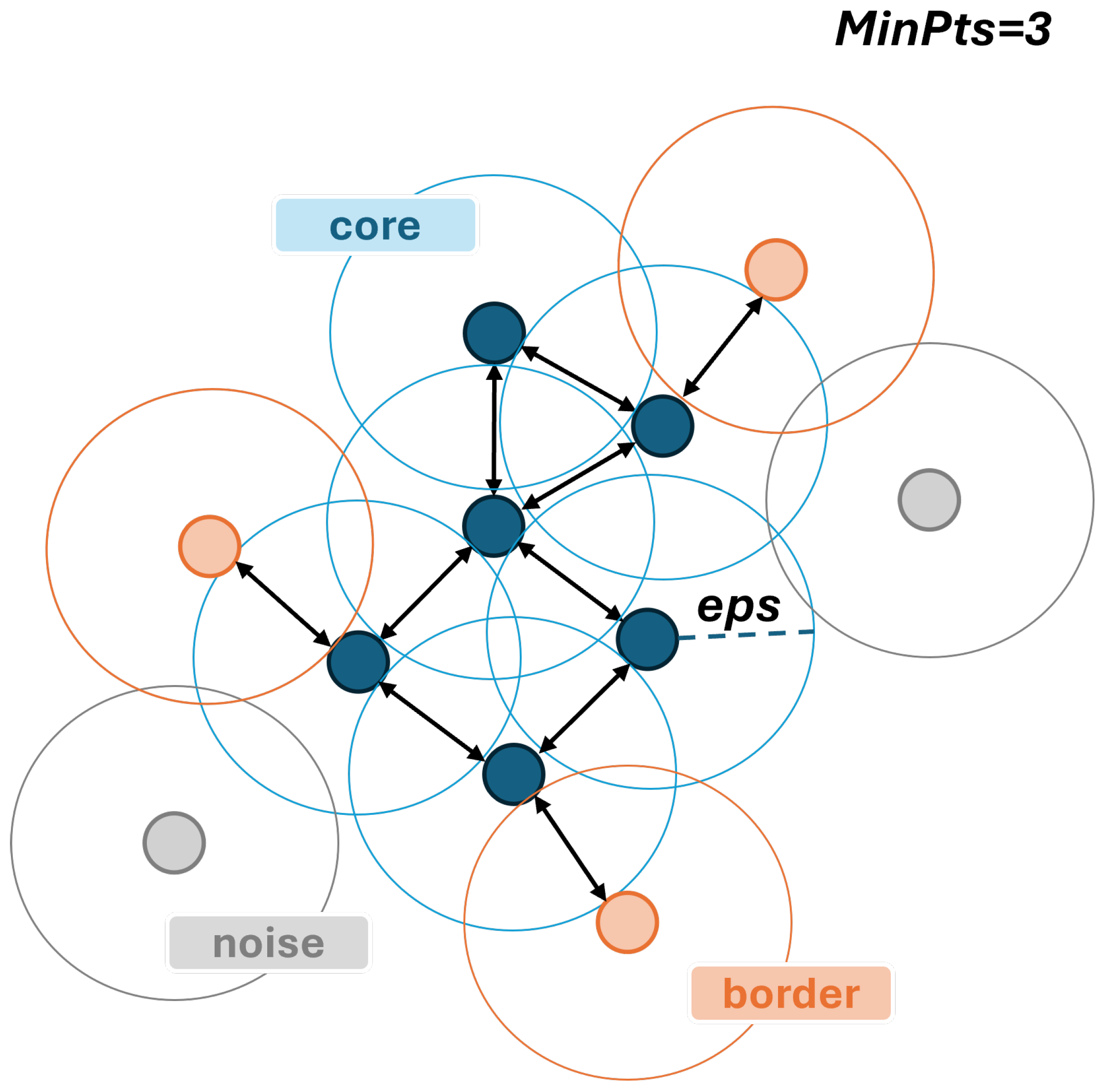
Recently, multiple Automatic Operational Modal Analysis (AOMA) strategies have been developed by making use of clustering approaches. Among these, the Density-Based Spatial Clustering of Applications with Noise (DBSCAN) algorithm has emerged as a promising tool because of its ability to identify and isolate non-physical poles, which enables a more robust identification of true structural modes. DBSCAN is a method that forms clusters by identifying regions of high point concentration and it operates on the basis of two main hyperparameters: ε , which defines the maximum distance between two points to be considered neighbors, and M i n P t s , the minimum number of neighboring points required to form a cluster.
As illustrated in Figure 2, DBSCAN categorizes data points into three types: core points, border points, and outliers. A core point is one that has at least M i n P t s other points within a radius defined by ε . Border points are those that do not meet the criteria to be core points themselves but lie within the neighborhood of a core point. Outliers are points that are neither core nor border points and do not belong to any dense region.
The clustering process begins by selecting an unlabeled point x i and checking how many points fall within its ε -neighborhood:
  • If x i is a core point, a new cluster is initiated. All points that are density-reachable from x i (i.e., connected through a chain of neighboring core points) are then included in the cluster.
  • If the number of neighboring points is less than M i n P t s , the point is classified as a border point if it lies within the neighborhood of a core point, or as an outlier point otherwise.
This process is repeated until all points have been assigned to a cluster or classified as an outlier.
The suitability of DBSCAN as a clustering method for automating Operational Modal Analysis lies primarily in its ability to operate without requiring prior knowledge of the number of clusters. Instead, it estimates this number autonomously by identifying densely populated regions in the data space. However, DBSCAN requires the specification of the minimum number of points constituting a cluster M i n P t s and the neighborhood radius ε . In the present work, these two parameters are tailored for the specific test case. Considering a certain system, a time series is selected as a reference and the hyperparameters of DBSCAN are manually tuned for this reference to ensure that the excited modes are optimally clustered. In particular, a grid search is conducted over predefined ranges for the DBSCAN parameters ε and M i n P t s . Each parameter pair is tested on the reference condition of the structure, and the resulting clustering performance is evaluated. Only the combinations that correctly identify the expected number of clusters and yield mean cluster frequencies sufficiently close to the target values for each mode are retained. From this subset of valid configurations, one parameter pair is then manually selected. In particular, the values employed in the following study are M i n P t s = 6 and ε = 0.1 (prior to applying DBSCAN, the frequency and damping values are normalized using z-score normalization). The selected parameters are then used to process all the acquired time series, resulting in an efficient clustering of the modal parameters. Once the poles have been grouped into clusters, the physical pole for each cluster is selected as the lowest-order pole in the longest sequence of stable poles as a design choice.

2.2. Graph Neural Networks

2.2.1. Graph Fundamentals

A graph (Figure 3) is a mathematical structure used to model relations between entities. It is defined as G = ( V , E ) , where:
  • V = { v 1 , , v N } is the set of nodes (or vertices);
  • E V × V is the set of edges, which encode relationships between nodes.
Graphs can be either directed, when the edges between the vertex pairs have a direction, or undirected, if the connections are symmetric. For simplicity, only undirected graphs will be considered in the following discussion. Figure 3 shows an example of an undirected graph consisting of 8 nodes and 11 connections. The blue dots represent the vertices, while the black lines indicate undirected edges between them.
The structure of a graph can be described using an adjacency matrix A R N × N , where A i j = 1 if there is a connection between node v i and node v j , and A i j = 0 otherwise. A degree matrix D R N × N can also be defined, which is a diagonal matrix where each element D i i represents the degree of node v i , i.e., the number of edges connected to it. Formally, D i i = j A i j .
While the adjacency matrix is often binary, indicating simply the presence or absence of an edge, it can also contain real-valued weights to represent the strength or significance of connections between nodes.
Each node v i is typically associated with a feature vector x i R F , and all node features are collected into the matrix X R N × F , where each row corresponds to a single node features.

2.2.2. Graph Convolutional Networks

Graph Neural Networks (GNNs) are a class of deep learning methods that operate on graphs, and thus are capable of handling data arranged on irregular, non-Euclidean domains, which allows them to model complex relational systems. GNNs are built on the principle of message passing (Figure 4), in which each node in a graph iteratively exchanges and aggregates information from its neighbors. Let v denote a generic node in the graph, N ( v ) its set of neighbors, h v ( l ) the feature vector of node v at layer l, and e u v the edge attributes between two neighbor nodes u and v. In general, the message passing process is decomposed into three sequential steps [33]:
  • Message preparation: Each neighboring node u N ( v ) generates a message m u v ( l ) to send to node v, which is typically a function of the source and target node embeddings, and optionally edge attributes:
    m u v ( l ) = MSG ( l ) h u ( l ) , h v ( l ) , e u v
  • Aggregation: Node v collects the messages coming from all its neighbors and combines them using a permutation-invariant aggregation function (e.g., sum and max):
    m v ( l ) = AGG ( l ) { m u v ( l ) : u N ( v ) }
  • Update: The node updates its own embedding by combining its previous state with the aggregated message
    h v ( l + 1 ) = UPD ( l ) h v ( l ) , m v ( l )
This three-step process is repeated across multiple layers of the network so that each node is able to incorporate information from increasingly distant portions of the graph.
Graph Convolutional Networks (GCNs) implement the message passing scheme using a specific aggregation strategy based on graph convolution [34]. In the basic GCN model, the aggregation is performed as a weighted sum of neighbor features, followed by a shared transformation [35]:
H ( l + 1 ) = σ D ^ 1 / 2 A ^ D ^ 1 / 2 H ( l ) W ( l )
where:
  • H ( l ) R N × P l is the matrix of node features at layer l ( P l number of node features);
  • A ^ = A + I is the adjacency matrix with self-loops;
  • D ^ is the degree matrix corresponding to A ^
  • W ( l ) R P l × P l + 1 is a trainable weight matrix;
  • σ is a non-linear activation function.
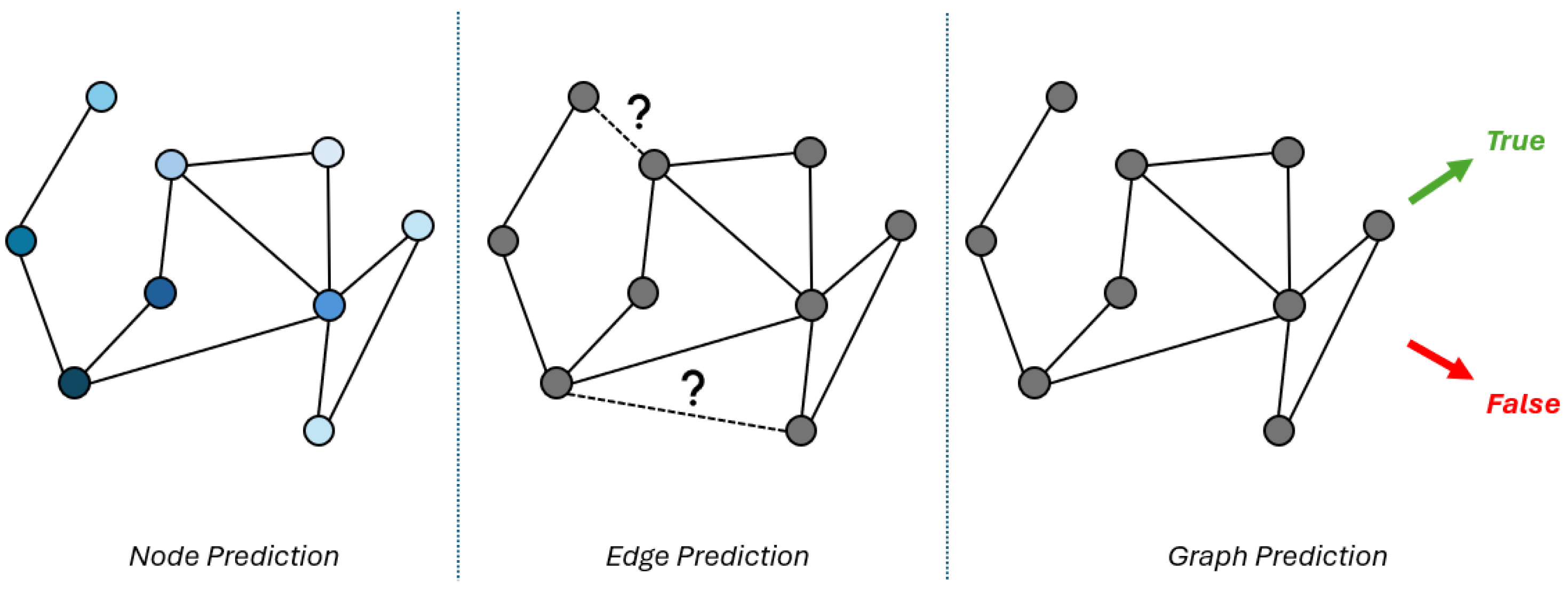
GNNs can be used for various prediction tasks [36], depending on the target level (Figure 5):
  • Node-level prediction: estimate the node embedding for each individual node in a graph;
  • Edge-level prediction: understand the relationship between entities in graphs and predict if two entities have a connection;
  • Graph-level prediction: predict a value associated with the entire graph.

3. Methodology

In this work, we consider a set of measurement points distributed across a structure equipped with strain sensors, such as strain gauges or Fiber Bragg Gratings (FBGs). Figure 6 shows an example of how a plate structure instrumented with a network of FBGs can be represented as a graph. On the left, the FBG sensors are arranged in a regular pattern along predefined lines on the plate surface. On the right, the corresponding graph representation is shown, where each sensor corresponds to a node and the edges represent spatial proximity or structural connectivity, enabling the construction of the adjacency matrix used in the GNN.
Assuming that the structure is subjected to a dynamic load that is randomly distributed both in space and time, it is possible to acquire a strain time history at each measurement point i, over a total of N t time steps. From these signals, Automatic Operational Modal Analysis techniques can be applied to estimate modal parameters: namely, natural frequencies, damping ratios, and strain mode shapes at each sensor location. This identification procedure can be performed both for a healthy baseline condition and for the current structural state. By comparing the two, one can quantify local variations in strain mode shapes across the sensor network.
Once the sensor network has been modeled as a graph, each node is assigned a set of features, which in this context correspond to the absolute differences in strain mode shapes between the healthy and current conditions, computed for a total of N m modes. Additional geometric information such as the Cartesian coordinates and local surface curvature along directions X, Y, and Z at each measurement point are also included as node attributes to enhance the representation. Therefore, the designed network is such that the input graph encapsulates both the topology of the sensor network and the observed modal variations. GNNs in this context can be trained to perform the following tasks:
  • Damage Detection: a graph-level prediction task in which the GNN classifies the entire structure as damaged or undamaged, based on the input node features.
  • Damage Localization: a node-level prediction task where the GNN estimates a probability distribution over the nodes, indicating the most likely locations of damage across the structure.
The general architecture of the proposed method is illustrated in Figure 7, and follows a modular approach, which separates the detection and localization tasks. Starting from the input features, namely the strain mode shape variations and the topological properties of the sensor network, a first Graph Neural Network (GNN1) performs a binary classification task to detect the presence of structural damage. If damage is detected, the same set of features is then passed to a second network (GNN2), which estimates the spatial distribution of the damage in a probabilistic way.

3.1. Dataset Generation

To train the GNN models, two distinct datasets containing modal information are generated. The first dataset is used for damage detection and includes both healthy and damaged structural conditions, as its task is to determine the presence or absence of damage. The second dataset, intended for damage localization, contains only damaged cases since its objective is to learn the relationship between spatial patterns of modal variations and the actual position of the damage. Both datasets are synthetic and are derived from a finite element model of the structure under investigation, in which damage is artificially introduced.
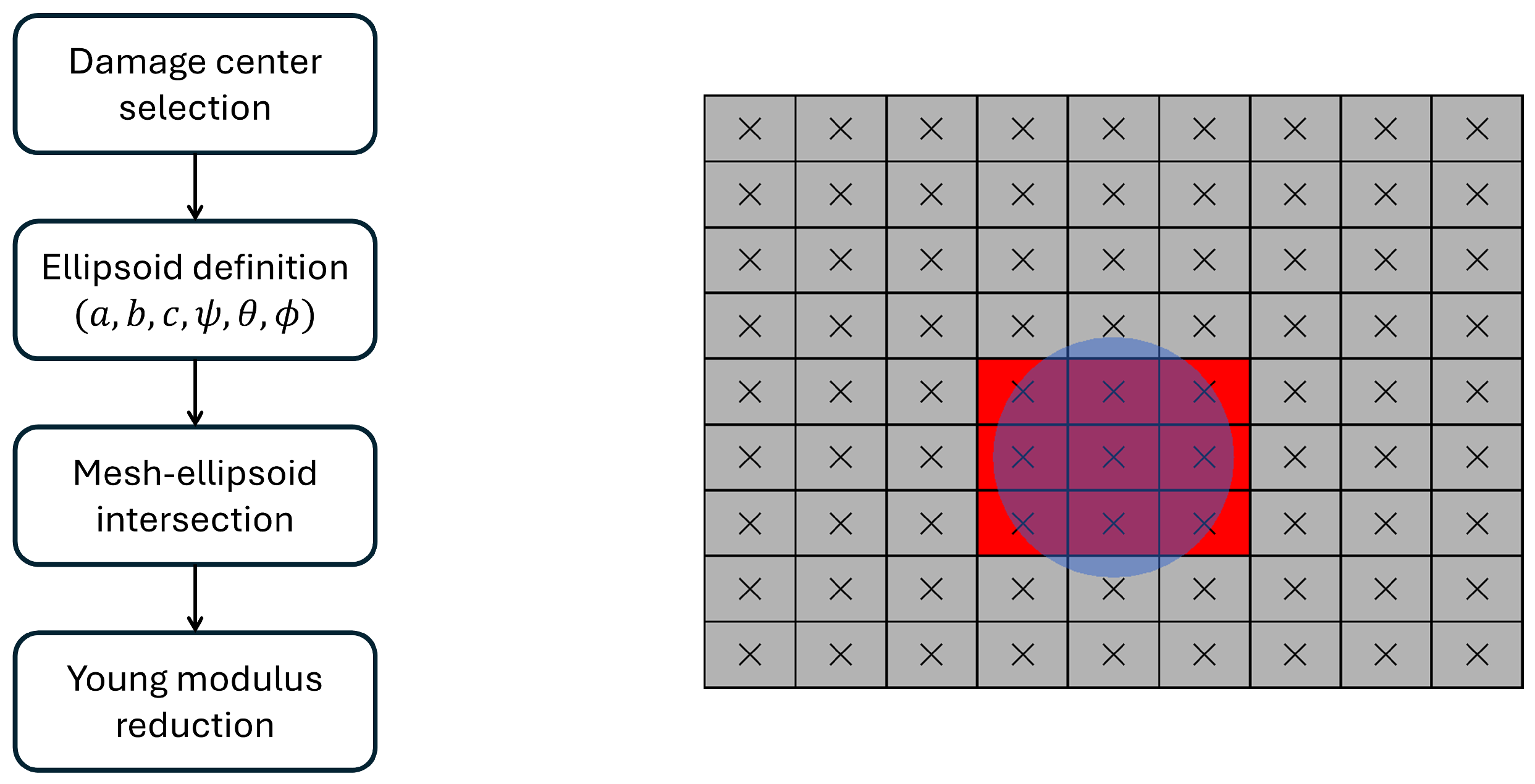
The process for generating a damaged FE model is illustrated in Figure 8 (left). The workflow begins with the random selection of a damage center from the centroids of the mesh elements. Around this center, an ellipsoid is constructed whose semi-axes a, b, and c are randomly sampled within predefined ranges to vary the size of the damaged region. The ellipsoid is then assigned a random spatial orientation, parameterized through three Euler angles ψ , θ , and ϕ . The actual definition of the damaged elements is obtained by intersecting the ellipsoid with the FE mesh. Specifically, all elements whose centroids fall inside the ellipsoid volume are classified as damaged. This procedure is visually clarified in Figure 8 (right), where grey elements represent the original FE mesh, black crosses indicate the centroids, and the blue ellipsoid defines the candidate damaged region. Elements whose centroids lie inside the ellipsoid are highlighted in red and designated as damaged. In this way, the ellipsoid acts as a spatial mask that selects a connected group of elements to which damage is applied. The abovementioned methodology allows for structural modularity to be taken into account. For example, if the structure is an aircraft wing and damage is to be introduced on the upper skin, only the elements belonging to that structural region are considered in the ellipsoid intersection, based on a prior segmentation of the mesh. This avoids unintentionally damaging elements of adjacent components, such as ribs or spars.
To ensure a sufficiently uniform distribution of damage locations across the structure, the damage centers are sampled using a blue noise strategy based on Poisson Disk Sampling [37]. Blue noise sampling places points randomly like white noise, but with the key difference that these points are more evenly distributed. This approach guarantees that selected points are well-spaced, avoiding excessive clustering and promoting coverage of all structural regions.
Once the set of damaged elements has been identified, the damage is applied by reducing the Young modulus in each direction E i i by a randomly selected amount as shown in Equation (16). In the case of composite structures, this reduction is applied to each orthotropic ply in the laminate:
E i i d a m a g e d = X E i i h e a l t h y , X ( 0 , 1 )
After defining the material properties, a random pressure field is generated in both time and space, and applied to the model. The excitation is band-limited to a frequency range [ 0 , f max ] . To ensure a consistent excitation and observability between the baseline and current configurations, the same spatial random distribution of the pressure field is used, while the temporal component is varied to simulate differences in operating conditions. A transient dynamic analysis is then performed to generate strain time histories. These signals are perturbed with a small amount of noise, and strain mode shapes are extracted using the Stochastic Subspace Identification method. Pole selection is automated via DBSCAN clustering of the stabilization diagram. As mentioned previously, for each physical mode identified, the representative pole is selected as the lowest-order solution from the longest consecutive sequence of stable poles within a cluster as a design choice.
For each damage case, the resulting strain mode shapes are stored, and their magnitude variation with respect to the healthy configuration is computed point-wise. The complete process for generating the damaged modal features is summarized in the flowchart shown in Figure 9. The colors indicate different categories: gray for input/output blocks, blue for computational steps, red for damaged states and green for healthy condition.
For healthy configurations, the same procedure is followed, except that no damage is introduced. In this case, the modal differences are evaluated between two distinct healthy configurations and are not identically zero due to the presence of noise and the randomness in the temporal excitation.

3.2. Detection GNN

The first neural network developed is designed to detect the presence of structural damage. It is composed of three stacked graph convolutional layers (described in Section 2.2.2), in which each node progressively update its features based on its neighbors. After each convolution, a ReLU activation function and dropout regularization are applied. Once the node-level features have been processed through the three layers, a global max pooling operation is performed. This operation extracts a single graph-level vector by retaining the maximum value per feature dimension:
h max = max i = 1 , , N p h i
where N p is the number of nodes in the graph, and h i is the feature vector of node i. The resulting vector is then passed through a final linear layer to produce a scalar output.
The network is trained using Binary Cross Entropy as the loss function, which is commonly used in binary classification problems [38]:
L BCE = y i log ( y ^ i ) + ( 1 y i ) log ( 1 y ^ i )
where y { 0 , 1 } is the ground truth label, and y ^ is the network output before the sigmoid activation. Since it is defined in terms of probabilities, the Binary Cross Entropy loss is dimensionless.
This formulation allows the network to output a continuous value, which is then interpreted as a probability of damage presence, and to be directly trained to minimize classification error.

3.3. Localization GNN

The second neural network developed in this work is a GNN specifically designed for damage localization. As in the previous case, the architecture is composed of a stack of three graph convolutional layers which process node-level features, followed by a decoder module, implemented here as a single-hidden-layer Multi-Layer Perceptron (MLP), which outputs a scalar value for each node representing the predicted probability of damage. As a result, the network produces a probability distribution over the graph, i.e., over the sensor network, indicating the most likely damage location. This output is trained against a target distribution defined from the known damage position. For each damage scenario, the geodesic distance ρ i (i.e., the distance across the structural domain) between each sensor node and the damage center is computed, and a decaying exponential function is applied:
z i = exp ρ i σ
where σ is a user-defined decay parameter that regulates how fast the influence of the damage attenuates across the structure. The values z i are then normalized to obtain a probability distribution:
π i = z i j = 1 N p z j
where N p is the number of sensor nodes. The resulting vector π serves as the ground-truth target distribution for the training of the network. To compare the predicted distribution π ^ with the target π , the Jensen–Shannon (JS) divergence is considered [39]:
L JS = 1 2 L KL ( π m ) + 1 2 L KL ( π ^ m ) with m = 1 2 ( π + π ^ )
where L KL is the Kullback–Leibler (KL) divergence loss defined as
L KL = i = 1 N p π i log π i π ^ i
The Jensen–Shannon divergence is dimensionless since it is derived from probability distributions.
We use the JS Divergence instead of the KL divergence because, in our case, the target distributions are constructed using exponentially decaying functions of geodesic distance, which leads to assigning near-zero values to several nodes. This may be a problem since KL becomes unstable when the predicted distribution assigns non-zero probability to components where the target distribution is zero (or vice versa). JS divergence avoids this issue by averaging the two distributions and computing the KL divergence with respect to the average, thus leading to more accurate results. Therefore, the JS Divergence loss function allow the network to learn spatial mappings between strain mode variations and likely damage positions and enables an interpretable localization based on the graph structure.

4. Results

4.1. Case Study

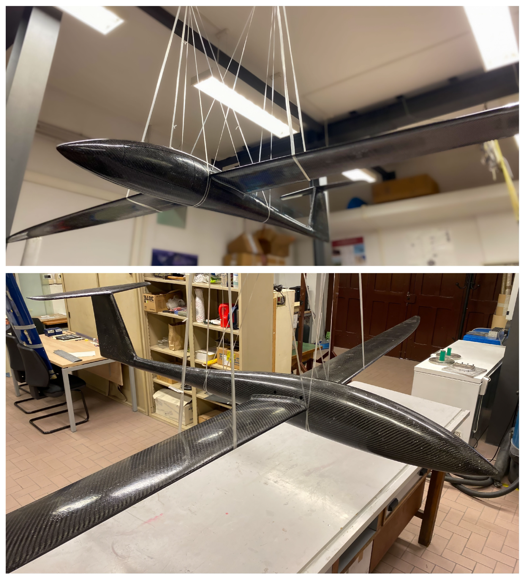
The case study considered in this work is a numerical finite element model of the wing belonging to a composite scaled glider manufactured at the Aerospace Composite Material Laboratory at the Department of Mechanical and Aerospace Engineering at Sapienza University of Rome [40]. This glider (shown in Figure 10) is a 1:5 scale reproduction of an existing standard class sailplane SZD-55-1 Nexus, but some changes were made to the original geometry in order to ease the manufacturing process.
This study concentrates solely on the numerical model of the glider wing, which is displayed in Figure 11 on the left. The wing consists of an upper and lower skin, 14 ribs, and a main spar located at 22% of the chord length. The first three ribs, situated near the clamped interface with the fuselage, are spaced 0.5 cm apart. The following three ribs are spaced 7 cm apart, while the remaining ones have a spacing of 14 cm. The skins and ribs are made of carbon fiber/epoxy composite using a twill weave fabric, whereas the internal spar is made of unidirectional carbon fiber/epoxy. Each structural component is composed of five plies, each 0.2 mm thick, all with a 0° orientation with respect to the others. The orthotropic material properties of the twill and unidirectional composites are reported in Table 1. The entire wing geometry is meshed using 4-node shell elements, resulting in a total of 67,806 elements and 66,967 nodes. The structure is constrained with clamped boundary conditions at the root. Therefore, the constraints are applied to the nodes located at the base of the main spar, which extends beyond the wing, and to the nodes of the first internal rib, which acts as a structural cap. A close-up of the constrained nodes is shown in orange in Figure 11 on the right.
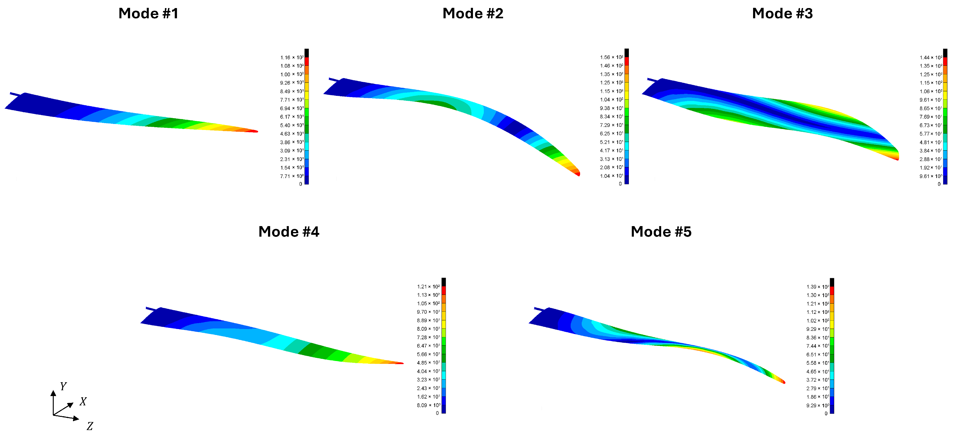
A preliminary modal analysis (using MSC Nastran SOL 103) is carried out on the wing to extract its first five modes, which are subsequently used for both damage detection and localization. The corresponding displacement mode shapes are shown in Figure 12. Mode #1 corresponds to the first bending mode; mode #2 represents the second bending mode; mode #3 exhibits a torsional deformation around the wing longitudinal axis, with opposite twisting between the leading and trailing edges; mode #4 corresponds to the first bending mode in the horizontal plane; and mode #5 appears as a higher-order flexural and torsional mode, with increased complexity in the twist distribution along the span. The natural frequencies related to these modes are summarized in Table 2.
To apply the previously described methodology, it is first necessary to define a set of measurement points where strain sensors will be placed. A total of 40 measurement points are used, equally distributed between the upper and lower skins of the wing. The placement follows this approach:
  • A number of spanwise sections is selected, seven for both the upper and lower skins, staggered along the wingspan;
  • A variable number of sensors is positioned on each section, decreasing from four near the wing root to one near the tip, reflecting the tapering of the wing’s cross-section.
In this study, a relatively uniform distribution of measurement points across the structure is adopted. However, in general, a more targeted layout could be considered, with a denser sensor placement in critical areas subject to high stress concentrations.
The aforementioned measurement points define the graph nodes; to fully specify the graph, the corresponding edges must also be established. This is achieved by first generating a triangular mesh that connects all points on the upper and lower surfaces separately. At the end of this initial process, two separate sets of connections are defined: one for the upper skin and one for the lower skin. To enable information exchange between them, additional edges are introduced. For each spanwise section, the nodes on the upper skin located near the leading and trailing edges are connected to the two closest nodes on the lower skin set boundary. All the edges of the graph are assigned a unitary weight. Figure 13 shows the graph associated with the sensor network described above. The measurement points on the upper skin are shown in blue, while those on the lower skin are shown in red. The black lines represent the graph connections.
Alternative connection strategies, such as a k-nearest neighbors graph and a fully connected graph, were also tested. Since both yielded lower performance in terms of damage detection and localization compared to the proposed structural topology-based approach, the corresponding results are omitted for brevity. It should be noted, however, that in general the adjacency matrix could be further optimized (for example, using Genetic Algorithms) to maximize the performance of the GNNs.
Once the set of measurement points is defined, transient analyses are carried out using the SOL112 solver in MSC Nastran, applying a spatially and temporally random force limited to the frequency band [0, 150] Hz, in order to excite the desired modes. The strain responses at the measurement points are recorded over 30,000 time steps with a sampling frequency of 400 Hz. These time signals are then processed with AOMA to extract the strain modes in the directions of the wingspan, generating the datasets used for training. While the strain sensors are placed only on the upper and lower skins, the damages are simulated on both the skins and the spar.

4.2. Detection Results

The damage classification network is trained on a dataset of 3500 samples, split into 70% for training, 15% for validation, and 15% for testing. Training is carried out for 300 epochs using mini-batches of 16 samples. The developed network employs 128 hidden states in each graph convolutional layer. The optimizer employed is AdamW [41], a variant of the widely used Adam algorithm, where weight decay does not accumulate in the momentum nor in variance. The training is performed using a fixed learning rate of 1 × 10 4 , without early stopping, and with a dropout rate of 0.2 applied to the hidden layers.
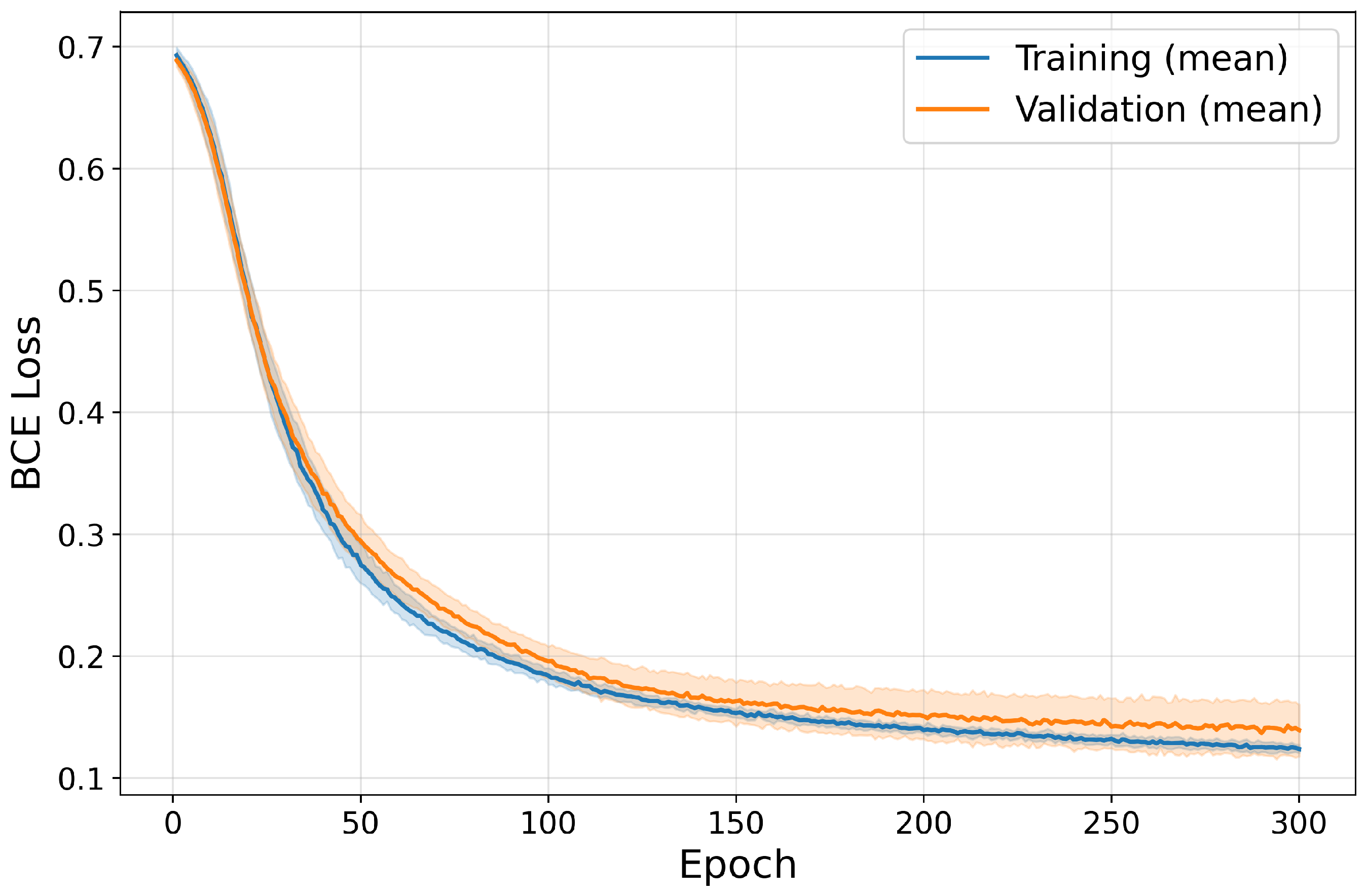
In Figure 14, the evolution of the BCE loss for the training set (blue curve) and the validation set (orange curve) is shown. The curves represent the mean trend obtained over 10 independent runs, while the shaded areas denote the corresponding ± 1 standard deviation intervals. Each run is performed with different random initializations of the training and test sets to demonstrate the reproducibility of the results. Both curves exhibit a consistent decreasing trend, which indicates that the model is learning effectively without overfitting. As expected, the validation loss remains slightly higher than the training loss, thus suggesting good generalization.
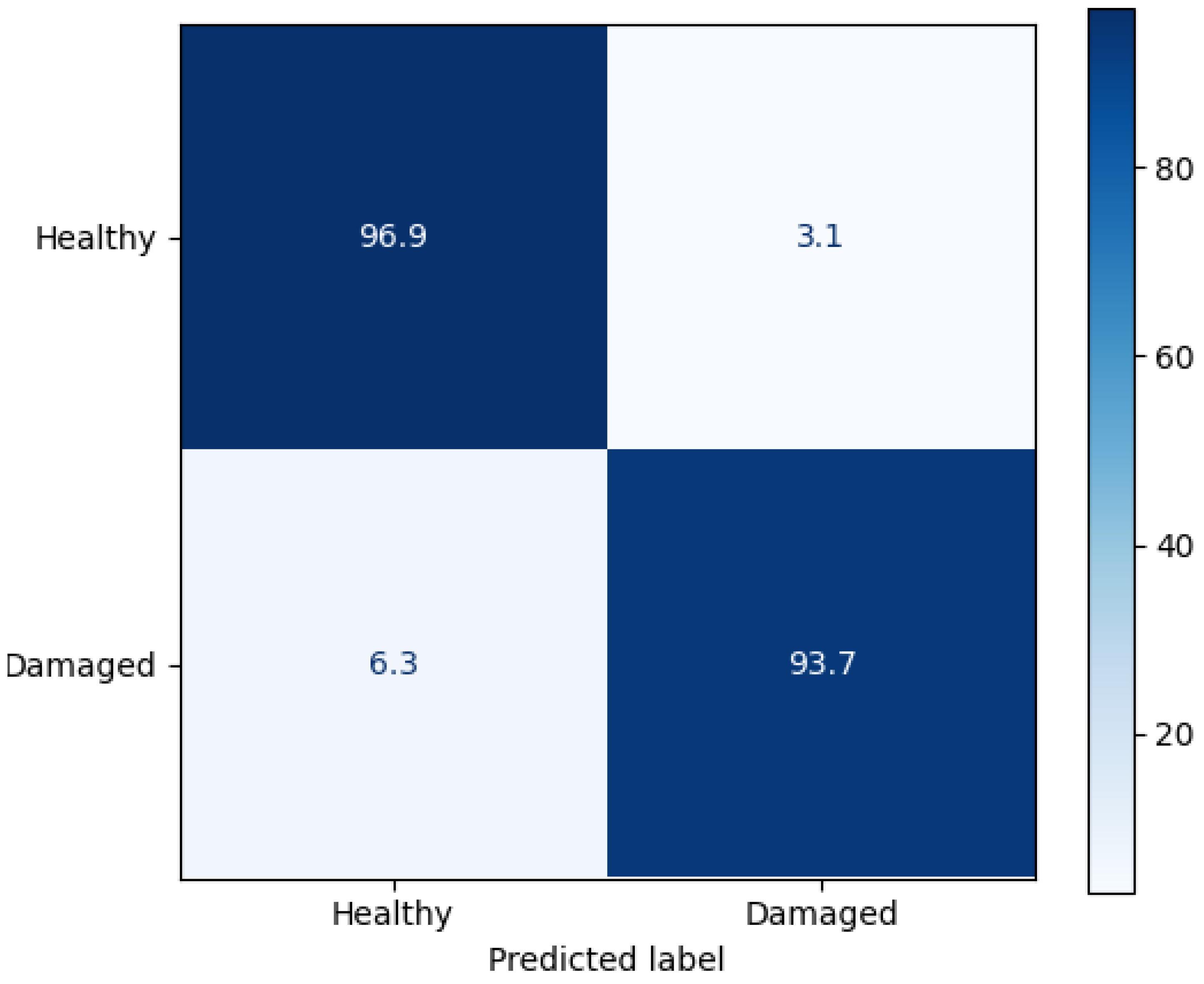
To assess the performance of the model, standard classification metrics are employed. The confusion matrix on the test set is reported in Figure 15, showing the number of true positives (TPs), true negatives (TNs), false positives (FPs), and false negatives (FNs). Since the network output is a continuous value between 0 and 1, the predictions are binarized using a threshold of 0.5. In particular, values above the threshold are classified as damaged, otherwise as healthy. As shown in the confusion matrix, the network achieves strong classification performance, with 3.1% of healthy samples incorrectly classified as damaged and 6.3% of damaged samples misclassified as healthy. The performance metrics (accuracy, precision, recall, and F1-score) are summarized in Table 3 along with the corresponding 95% confidence intervals (CIs) computed using a bootstrapping approach [42].
Since such metrics depend on the choice of classification threshold (here fixed at 0.5), which is often chosen arbitrarily and can significantly affect the evaluation process, it is common to evaluate the binary classifier robustness using the Receiver Operating Characteristic (ROC) curve, which for different threshold values plots the True Positive Rate (TPR) against the False Positive Rate (FPR), defined as
FPR = FP FP + TN
In particular, to compute the ROC curve, the classification threshold is gradually varied from 0 to 1. At each step, values above the threshold are classified as positives. If these predicted positives fall within the region corresponding to the actual damage, they are considered true positives (i.e., correct detections); otherwise, they are treated as false positives (i.e., false alarms). For each threshold, the True Positive Rate and False Positive Rate are computed, resulting in a single point on the ROC curve. By collecting all such points, the full ROC curve for the test set is constructed. The ROC for this network is presented in Figure 16. The Area Under the ROC Curve (AUC) summarizes the classifier performance in a single scalar value that ranges from 0 to 1. An AUC of 0.5 corresponds to random guessing, while an AUC of 1.0 indicates perfect discrimination. The AUC can be interpreted as the probability that the classifier ranks a randomly chosen positive instance higher than a randomly chosen negative one. In this case study, the AUC obtained is 0.97, thus indicating a highly efficient classification.
An analysis of the importance of the input features on the classification performance is also carried out, focusing in particular on the AUC metric. An ablation study is therefore performed on the input features, comparing the effect of using both modal and geometric features against using only the modal ones. Obviously, providing geometric data alone does not give any indication about the presence of damage and is therefore not considered. The obtained results are reported in Table 4, where the AUC values and the corresponding confidence intervals are listed for each case. The inclusion of geometric features increases the AUC from 0.958 to 0.970, indicating a modest improvement.

4.3. Localization Results

The neural network designed for damage localization is trained on a dataset composed of 3500 damaged samples, featuring damages with varying sizes, orientations (defined by the ellipsoid Euler angles), and intensities. Of these, 70% is used for training, 15% for validation, and the remaining 15% for testing.
In defining the output probability at each sensor location, based on its geodesic distance from the damaged area (as described by Equation (19)), the parameter σ is set to 5 cm. This value is selected through a trial-and-error process guided by insights from the FE model of the structure. The network architecture consists of three graph convolutional layers with 256, 128, and 64 hidden states, respectively. These are followed by a multi-layer perceptron (MLP) with 16 hidden neurons, which acts as a decoder that maps the output to a scalar value for each vertex of the graph. The optimizer used is again AdamW, and the network is trained for 300 epochs using batches of 16 samples. The training is performed using a fixed learning rate of 1 × 10 3 , without early stopping, and with a dropout rate of 0.2 applied to the hidden layers. The evolution of the training and validation loss (measured by the Jensen–Shannon divergence) is shown in Figure 17, where the blue and orange curves represent the mean trend over 10 independent runs, while the shaded areas denote the corresponding ± 1 standard deviation intervals.
As previously mentioned, the network outputs a probability distribution that assigns higher values to measurement points closer to the damaged area. An example of a predicted damage distribution is shown in Figure 18, where it is compared with the corresponding “ground truth” distribution used during training. The dots represent the measurement points (graph nodes), and their associated color indicates the predicted damage probability; the black cross marks the location of the actual damage center.
To evaluate the performance of the network, the Earth Mover’s Distance (EMD), a widely used metric for quantifying differences between probability distributions, is employed. To understand this quantity, one can think of a distribution as a pile of mass (the probability) spread across a set of locations (the nodes of the graph), and transforming one distribution into another corresponds to reshaping the pile so that it matches the second configuration. The cost of moving a unit of mass from one location to another is proportional to the ground distance between them. EMD measures the minimum total cost required to move the entire mass of one distribution to match the other. Mathematically, this is formulated as an instance of the transportation problem: given two non-negative distributions P and Q with equal total mass and a ground distance matrix D, EMD is defined as
EMD ( P , Q ) = min F i , j F i j D i j
where F i j represents the amount of mass moved from location i in P to location j in Q, and the optimization is subject to flow conservation constraints that ensure the outgoing mass from P and the incoming mass to Q match the original distributions. In our case P is the predicted damage distribution, Q is the “ground truth” damage distribution, and D is a matrix which contains the distances between the measurement points.
Figure 19 (top) shows the predicted damage probability distribution for one of the best-performing test samples in terms of Earth Mover’s Distance (EMD = 6.71 mm). As can be seen, such a low EMD value corresponds to an almost perfect spatial match between the predicted and actual damage probability distributions. Figure 19 (bottom), on the other hand, presents one of the worst cases (EMD = 295.61 mm). Despite the network correctly identifying the location of the maximum damage probability, the prediction is much more uncertain: the values are significantly lower than expected and are spatially more dispersed. As a result, the centroid of the predicted distribution is substantially displaced from the actual damage center, requiring greater effort to align the two distributions.
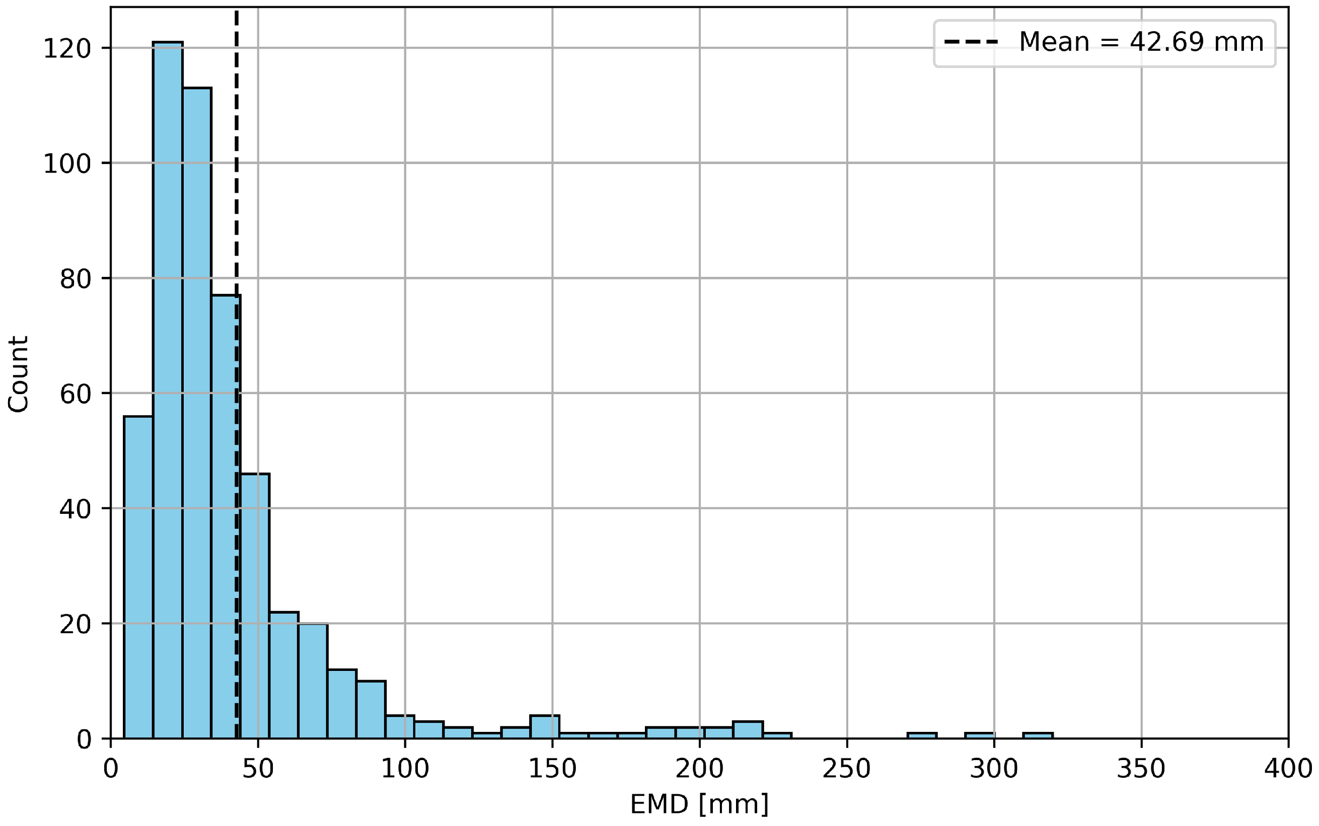
Figure 20 displays the histogram of EMD values across the test set. The distribution is skewed towards low values, with only a few cases exceeding 150 mm. Errors below 50 mm (≈3% of the wingspan) could be considered excellent, between 50 and 100 mm (≈3–7%) good, and in the 100–150 mm range (≈7–10%) still acceptable for guiding inspections. Conversely, values above 150 mm (>10%) indicate poor localization accuracy and would be of limited practical use in maintenance. The average EMD is 42.69 mm, which considering a wing span of 1500 mm is remarkably small and indicates a high level of agreement between the predicted and ground truth distributions. The results in terms of mean, standard deviation, and confidence intervals of the distribution (computed via bootstrapping) are reported in Table 5. As in the detection task, the importance of the different input features is also assessed through an ablation analysis, which is also included in Table 5. In particular, the effect on the mean and standard deviation of the EMD is evaluated by comparing the full feature set (modal variations and geometric properties at the measurement points) against the use of modal variations only. As can be observed, the inclusion of geometric coordinates and local curvature provides a significant contribution to the localization capability, roughly halving the mean localization error.
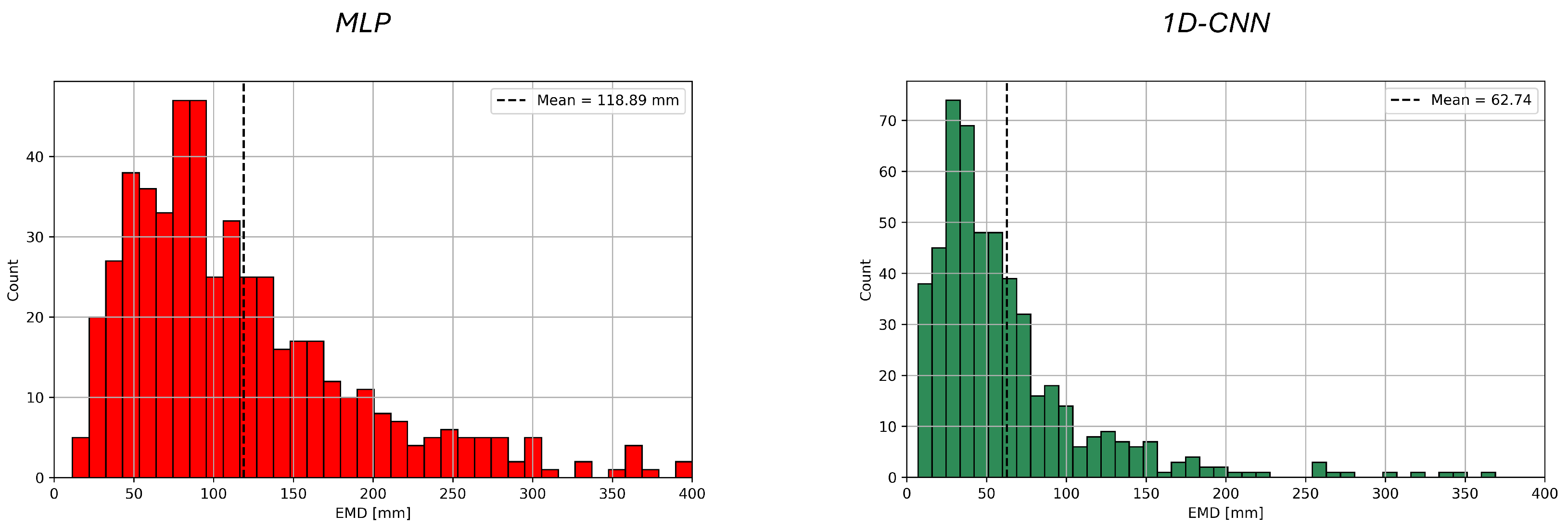
The localization performance of the proposed GNN is further compared against other data-driven baseline configurations. In particular, we consider a fully connected MLP and a 1D-CNN, both designed with approximately the same number of learnable parameters as the GNN. The inclusion of the 1D-CNN is motivated by its ability to exploit local correlations in the input data, while still being less dependent on an explicitly defined graph structure. However, since the sensor layout is inherently irregular and three-dimensional, mapping it onto a one-dimensional sequence requires an arbitrary ordering strategy. In this work, a “zigzag” pattern is adopted, which is shown in Figure 21. The CNN employs a kernel size of 5 to capture local dependencies along this sequence. The resulting EMD histograms for the MLP and 1D-CNN are shown in Figure 22. While the MLP is still able to generalize to some extent, its performance is considerably worse than the GNN as indicated by the broader distribution and higher mean EMD values. The 1D-CNN performs better than the MLP, narrowing the error distribution and reducing the average localization error, yet it still falls short of the GNN, which remains superior thanks to its ability to explicitly leverage the whole network topology. The statistical parameters of the EMD of the three methods (mean, standard deviation, and 95% confidence intervals of the mean) are summarized in Table 6.

5. Conclusions

In conclusion, this work proposes an innovative methodology based on Graph Neural Networks, where the graph represents the sensor network used for Structural Health Monitoring in aerospace structures. Strain time histories collected from a set of measurement points are processed using Automated Operational Modal Analysis to extract strain mode shapes, which are then provided as input to different GNN architectures, along with topological information, to perform both damage detection and localization on the system. Damage localization is carried out by predicting a probability distribution based on the geodesic distance between each sensor and the damaged area, enabling a relatively accurate estimation of the damage location. Both networks are tested on a case study involving a composite wing instrumented with 40 strain sensors (e.g., 40 FBGs), demonstrating excellent monitoring capabilities. The localization performance is also compared with that of a classical fully connected network and a convolutional network. By leveraging the inherent topology of the sensor network, the proposed GNN framework achieves approximately one-third of the mean localization error of the fully connected baseline, and reduces the error by around 30% compared to the CNN. Thus, although the GNN exhibits a higher architectural complexity, this leads to significantly better performance and improved generalization capabilities for this type of problem.
In addition to these promising numerical results, it is important to consider practical aspects that may influence the applicability of the proposed framework in real-world SHM scenarios. Possible factors include inference time, sensor synchronization, and sampling requirements. Inference time is mainly affected by the application of the AOMA procedure, whose computational cost grows with the number of acquired samples, the time shift k, and the maximum system order. In practice, however, periodic updates at intervals of the order of some seconds could be sufficient depending on the application. Sensor synchronization could be managed using FBG sensors interrogated through dedicated multiplexing units, which are commercially available and ensure precise timing. These sensors are also lightweight and can be embedded into composite structures, which is advantageous in the aerospace field. The required sampling frequency instead depends on the number of modes to be extracted: for instance, considering only the first 5–6 global modes of the aircraft may require sampling rates of just a few hundred Hz, as adopted in this study.
Some aspects of the proposed framework could also be extended in future works to improve robustness and applicability. In this study, the damage is modeled isotropically by uniformly reducing the Young modulus in all directions. Therefore, future developments could consider orthotropic damage scenarios, as explored in [5,43], along with a more representative synthetic damage dataset. Additional future analyses could focus on investigating how sensor misplacements or sensor faults may affect the performance of the proposed framework, particularly since it is shown that the inclusion of both geometric and modal features provides advantages in both classification and localization. Another key development will involve experimental validation on a physical structure, following the creation of an updated FE model accurately reflecting the real system, in order to assess the impact of using synthetic data in practical applications.

Author Contributions

Conceptualization, E.D.P. and L.L.; methodology, E.D.P.; software, E.D.P.; validation, E.D.P.; formal analysis, E.D.P.; investigation, E.D.P.; resources, L.L.; data curation, E.D.P.; writing—original draft preparation, E.D.P. and L.L.; writing—review and editing, E.D.P. and L.L.; visualization, E.D.P.; supervision, L.L.; project administration, L.L. All authors have read and agreed to the published version of the manuscript.

Funding

This research received no external funding.

Institutional Review Board Statement

Not applicable.

Informed Consent Statement

Not applicable.

Data Availability Statement

The data are contained within the article.

Acknowledgments

This work is part of the research activities developed by the authors within the framework of PNRR: CN4 “Sustainable Mobility Center”—SPOKE 1 “Air Mobility”.

Conflicts of Interest

The authors declare no conflicts of interest.

References

  1. Giurgiutiu, V.; Soutis, C. Enhanced composites integrity through structural health monitoring. Appl. Compos. Mater. 2012, 19, 813–829. [Google Scholar] [CrossRef]
  2. Dong, T.; Kim, N.H. Cost-effectiveness of structural health monitoring in fuselage maintenance of the civil aviation industry. Aerospace 2018, 5, 87. [Google Scholar] [CrossRef]
  3. Barazanchy, D.; Martinez, M.; Rocha, B.; Yanishevsky, M. A hybrid structural health monitoring system for the detection and localization of damage in composite structures. J. Sensors 2014, 2014, 109403. [Google Scholar] [CrossRef]
  4. Rytter, A. Vibrational Based Inspection of Civil Engineering Structures. Ph.D. Thesis, Aalborg University, Aalborg, Denmark, 1993. [Google Scholar]
  5. Pagani, A.; Enea, M. Displacement and strain data-driven damage detection in multi-component and heterogeneous composite structures. Mech. Adv. Mater. Struct. 2024, 31, 2053–2068. [Google Scholar] [CrossRef]
  6. Sonker, M.; Shanker, R. Enhanced diagnostic approach for multiple damage detection and severity evaluation through EMI-based sensing and artificial neural network model. Asian J. Civ. Eng. 2025, 26, 747–760. [Google Scholar] [CrossRef]
  7. Facciotto, N.; Martinez, M.; Troiani, E. Source identification and classification of acoustic emission signals by a SHAZAM-inspired Pattern Recognition Algorithm. In Proceedings of the International Workshop on Structural Health Monitoring (IWSHM 2017), Palo Alto, CA, USA, 12–14 September 2017; Volume 12783. [Google Scholar]
  8. De Fenza, A.; Sorrentino, A.; Vitiello, P. Application of Artificial Neural Networks and Probability Ellipse methods for damage detection using Lamb waves. Compos. Struct. 2015, 133, 390–403. [Google Scholar] [CrossRef]
  9. Pirrotta, C.; Gueli, A.M.; Trigona, C.; Imposa, S. Coherence Analysis for Vibration Monitoring Under High Variability Conditions: Constraints for Cultural Heritage Preventive Conservation. J. Sens. Actuator Netw. 2025, 14, 45. [Google Scholar] [CrossRef]
  10. Fan, W.; Qiao, P. Vibration-based damage identification methods: A review and comparative study. Struct. Health Monit. 2011, 10, 83–111. [Google Scholar] [CrossRef]
  11. Azimi, M.; Eslamlou, A.D.; Pekcan, G. Data-driven structural health monitoring and damage detection through deep learning: State-of-the-art review. Sensors 2020, 20, 2778. [Google Scholar] [CrossRef]
  12. Chen, Z.; Huang, H.Z.; Wu, J.; Wang, Y. Zero-faulty sample machinery fault detection via relation network with out-of-distribution data augmentation. Eng. Appl. Artif. Intell. 2025, 141, 109753. [Google Scholar] [CrossRef]
  13. Chen, Z.; Huang, H.Z.; Deng, Z.; Wu, J. Shrinkage mamba relation network with out-of-distribution data augmentation for rotating machinery fault detection and localization under zero-faulty data. Mech. Syst. Signal Process. 2025, 224, 112145. [Google Scholar] [CrossRef]
  14. Sahin, M.; Shenoi, R. Quantification and localisation of damage in beam-like structures by using artificial neural networks with experimental validation. Eng. Struct. 2003, 25, 1785–1802. [Google Scholar] [CrossRef]
  15. Pagani, A.; Enea, M.; Carrera, E. Component-wise damage detection by neural networks and refined FEs training. J. Sound Vib. 2021, 509, 116255. [Google Scholar] [CrossRef]
  16. Rao, P.S.; Mahendra, N. Vibration based damage identification method for cantilever beam using artificial neural network. In Proceedings of the International Conference on Experimental Vibration Analysis for Civil Engineering Structures, La Jolla, CA, USA, 12–14 July 2017; Springer: Berlin/Heidelberg, Germany, 2017; pp. 85–93. [Google Scholar]
  17. Padil, K.H.; Bakhary, N.; Abdulkareem, M.; Li, J.; Hao, H. Non-probabilistic method to consider uncertainties in frequency response function for vibration-based damage detection using Artificial Neural Network. J. Sound Vib. 2020, 467, 115069. [Google Scholar] [CrossRef]
  18. Zhong, K.; Teng, S.; Liu, G.; Chen, G.; Cui, F. Structural damage features extracted by convolutional neural networks from mode shapes. Appl. Sci. 2020, 10, 4247. [Google Scholar] [CrossRef]
  19. Nguyen, D.H.; Wahab, M.A. Damage detection in slab structures based on two-dimensional curvature mode shape method and Faster R-CNN. Adv. Eng. Softw. 2023, 176, 103371. [Google Scholar] [CrossRef]
  20. Duran, B.; Emory, D.; Azam, Y.E.; Linzell, D.G. A novel CNN architecture for robust structural damage identification via strain measurements and its validation via full-scale experiments. Measurement 2025, 239, 115393. [Google Scholar] [CrossRef]
  21. Wu, Z.; Pan, S.; Chen, F.; Long, G.; Zhang, C.; Yu, P.S. A comprehensive survey on graph neural networks. IEEE Trans. Neural Networks Learn. Syst. 2020, 32, 4–24. [Google Scholar] [CrossRef]
  22. Miele, E.S.; Bonacina, F.; Corsini, A. Deep anomaly detection in horizontal axis wind turbines using graph convolutional autoencoders for multivariate time series. Energy AI 2022, 8, 100145. [Google Scholar] [CrossRef]
  23. Kim, M.; Song, J.; Kim, C.W. Near-real-time damage identification under vehicle loads using dynamic graph neural network based on proper orthogonal decomposition. Mech. Syst. Signal Process. 2025, 224, 112175. [Google Scholar] [CrossRef]
  24. Son, H.; Pham, V.T.; Jang, Y.; Kim, S.E. Damage localization and severity assessment of a cable-stayed bridge using a message passing neural network. Sensors 2021, 21, 3118. [Google Scholar] [CrossRef] [PubMed]
  25. Jiang, C.; Chen, N.Z. G-Twin: Graph neural network-based digital twin for real-time and high-fidelity structural health monitoring for offshore wind turbines. Mar. Struct. 2025, 103, 103813. [Google Scholar] [CrossRef]
  26. Pollet, M.; Shepherd, P.; Hawkins, W.; Costa, E. Fast Structural Analysis of Concrete Thin-Shells Using Deep Learning. Preprint 2025. [Google Scholar] [CrossRef]
  27. Cui, H.; Du, H.; Zhao, F.; Hong, M. Damage identification in a plate structure based on a cross-direction strain measurement method. Measurement 2020, 158, 107714. [Google Scholar] [CrossRef]
  28. Peeters, B.; De Troyer, T.; Guillaume, P.; Van der Auweraer, H. In-flight modal analysis-a comparison between sweep and turbulence excitation. In Proceedings of the ISMA2006: International Conference on Noise and Vibration Engineering, Heverlee, Belgium, 18–20 September 2006; pp. 1627–1641. [Google Scholar]
  29. Brincker, R.; Andersen, P. Understanding stochastic subspace identification. In Proceedings of the IMAC-XXIV: A Conference & Exposition on Structural Dynamics, St Louis, MI, USA, 30 January–2 February 2006; Society for Experimental Mechanics: Bethel, CT, USA, 2006. [Google Scholar]
  30. Civera, M.; Sibille, L.; Fragonara, L.Z.; Ceravolo, R. A DBSCAN-based automated operational modal analysis algorithm for bridge monitoring. Measurement 2023, 208, 112451. [Google Scholar] [CrossRef]
  31. Wu, C.; Liu, H.; Qin, X.; Wang, J. Stabilization diagrams to distinguish physical modes and spurious modes for structural parameter identification. J. Vibroengineering 2017, 19, 2777–2794. [Google Scholar] [CrossRef]
  32. McLachlan, G.; Ng, S.; Peel, D. On clustering by mixture models. In Exploratory Data Analysis in Empirical Research, Proceedings of the 25th Annual Conference of the Gesellschaft für Klassifikation eV, Munich, Germany, 14–16 March 2001; Springer: Berlin/Heidelberg, Germany, 2003; pp. 141–148. [Google Scholar]
  33. Gilmer, J.; Schoenholz, S.S.; Riley, P.F.; Vinyals, O.; Dahl, G.E. Neural message passing for quantum chemistry. In Proceedings of the International Conference on Machine Learning, PMLR, Sydney, Australia, 6–11 August 2017; pp. 1263–1272. [Google Scholar]
  34. Kipf, T.N.; Welling, M. Semi-supervised classification with graph convolutional networks. arXiv 2016, arXiv:1609.02907. [Google Scholar]
  35. Bessadok, A.; Mahjoub, M.A.; Rekik, I. Graph neural networks in network neuroscience. IEEE Trans. Pattern Anal. Mach. Intell. 2022, 45, 5833–5848. [Google Scholar] [CrossRef]
  36. Corso, G.; Stark, H.; Jegelka, S.; Jaakkola, T.; Barzilay, R. Graph neural networks. Nat. Rev. Methods Prim. 2024, 4, 17. [Google Scholar] [CrossRef]
  37. Wang, T. Poisson-disk sampling: Theory and applications. In Encyclopedia of Computer Graphics and Games; Springer: Berlin/Heidelberg, Germany, 2024; pp. 1424–1431. [Google Scholar]
  38. Ruby, U.; Yendapalli, V. Binary cross entropy with deep learning technique for image classification. Int. J. Adv. Trends Comput. Sci. Eng. 2020, 9, 5393–5397. [Google Scholar] [CrossRef]
  39. Fuglede, B.; Topsoe, F. Jensen-Shannon divergence and Hilbert space embedding. In Proceedings of the International Symposium on Information Theory, ISIT, Washington, DC, USA, 27 June–2 July 2004; p. 31. [Google Scholar]
  40. Sbarra, R.G.; Del Priore, E.; Coppotelli, G.; Lampani, L.; Pasquali, M. On the Use of Fiber Optic Sensors and Operational Modal Analysis for Structural Health Monitoring in Aerospace Structures. In Proceedings of the ISMA 2024—International Conference on Noise and Vibration Engineering and USD 2024—International Conference on Uncertainty in Structural Dynamics, Leuven, Belgium, 9–11 September 2024; pp. 2346–2358. [Google Scholar]
  41. Llugsi, R.; El Yacoubi, S.; Fontaine, A.; Lupera, P. Comparison between Adam, AdaMax and Adam W optimizers to implement a Weather Forecast based on Neural Networks for the Andean city of Quito. In Proceedings of the 2021 IEEE Fifth Ecuador Technical Chapters Meeting (ETCM), Cuenca, Ecuador, 12 October 2021; pp. 1–6. [Google Scholar]
  42. Michelucci, U.; Venturini, F. Estimating neural network’s performance with bootstrap: A tutorial. Mach. Learn. Knowl. Extr. 2021, 3, 357–373. [Google Scholar] [CrossRef]
  43. Shahbazi, M. An Efficient Virtual Testing Framework to Simulate the Progression of Damage in Notched Composite Laminates. Ph.D. Thesis, University of British Columbia, Vancouver, BC, Canada, 2017. [Google Scholar]
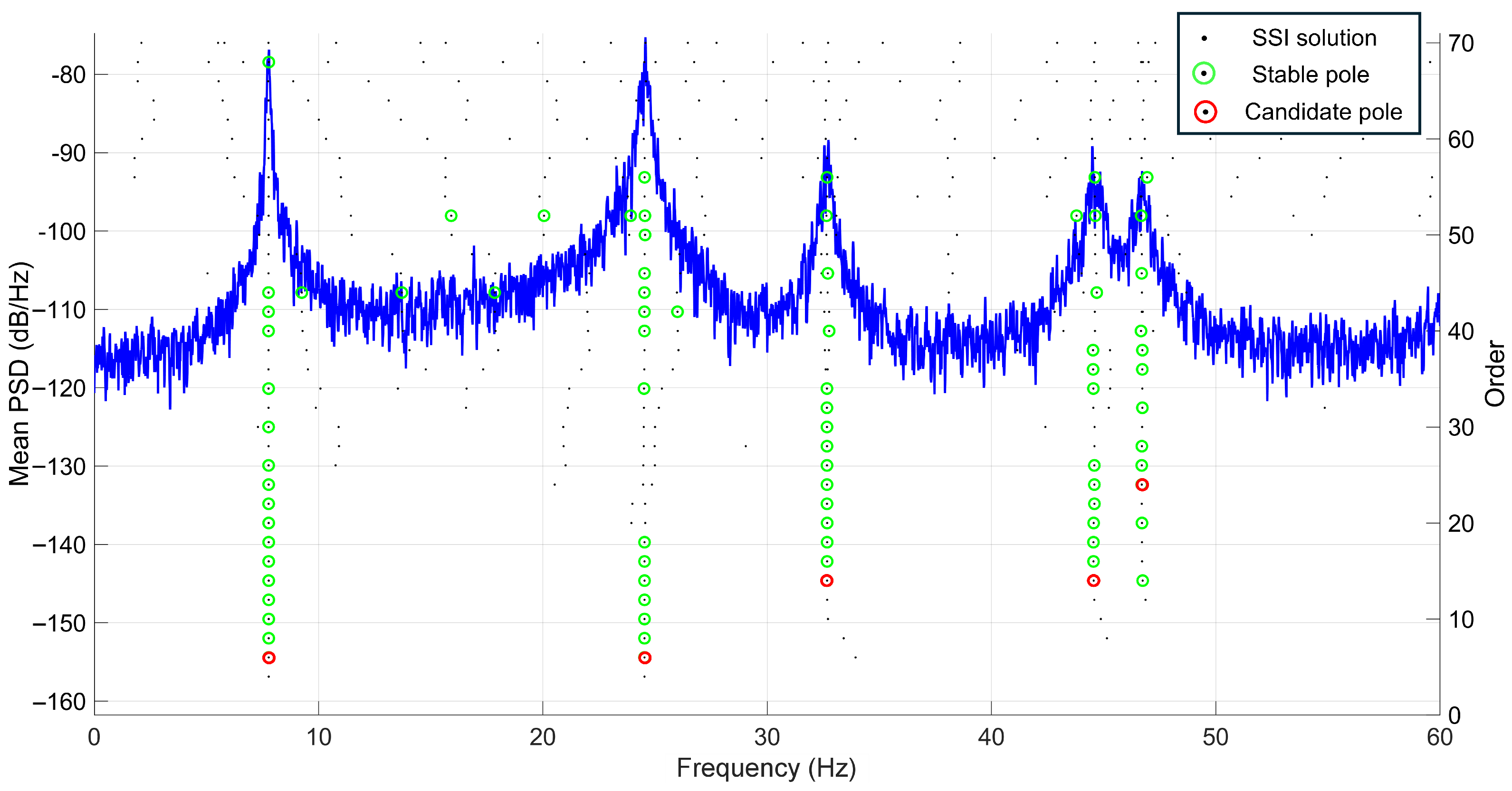
Figure 1. Stabilization diagram: black dots are the SSI solutions, green dots indicate stable poles, and red dots represent candidate poles for mode selection (system orders range from 4 to 70, with solutions shown every 2 orders).
Jsan 14 00089 g001
Figure 2. Classification of points according to the DBSCAN algorithm.
Jsan 14 00089 g002
Figure 3. Example of an undirected graph with 8 nodes and 11 edges.
Jsan 14 00089 g003
Figure 4. Message passing process for a GNN.
Jsan 14 00089 g004
Figure 5. Typical tasks of a GNN.
Jsan 14 00089 g005
Figure 6. Graph-based representation of a sensor network on a plate structure.
Jsan 14 00089 g006
Figure 7. Flowchart of the proposed GNN-based framework.
Jsan 14 00089 g007
Figure 8. Flowchart of the damaged FE model definition process (left) and example of the selection of the damaged elements by intersection with an ellipsoid (right).
Jsan 14 00089 g008
Figure 9. Procedure for computing damaged strain modes variation.
Jsan 14 00089 g009
Figure 10. Scaled composite glider.
Jsan 14 00089 g010
Figure 11. External and internal geometry of the composite wing (left) and close-up of the constrained nodes in orange (right).
Jsan 14 00089 g011
Figure 12. Displacement mode shapes 1–5 of the wing.
Jsan 14 00089 g012
Figure 13. Graph of the wing sensor network.
Jsan 14 00089 g013
Figure 14. Mean trend of training and validation loss for the classification GNN.
Jsan 14 00089 g014
Figure 15. Confusion matrix (in %) of the classification network.
Jsan 14 00089 g015
Figure 16. Receiver Operating Characteristic curve of the detection network.
Jsan 14 00089 g016
Figure 17. Mean trend of training and validation loss for the localization GNN.
Jsan 14 00089 g017
Figure 18. Example of damage probability distribution: on the left the GNN prediction and “ground truth” on the right.
Jsan 14 00089 g018
Figure 19. Low EMD (top) and high EMD (bottom) damage probabilities.
Jsan 14 00089 g019
Figure 20. Histogram of the EMD for the proposed GNN framework.
Jsan 14 00089 g020
Figure 21. Measurement point order for the 1D-CNN application.
Jsan 14 00089 g021
Figure 22. Histograms of the EMD for the MLP (left) and 1D-CNN (right).
Jsan 14 00089 g022
Table 1. Orthotropic properties of the twill and unidirectional composite plies.
Material E 11 [MPa] E 22 [MPa] G 12 [MPa] ν 12 Density [kg/mm3]
Twill47,00047,00034200.062 1.24 × 10 9
Unidirectional141,00011,00055000.280 1.52 × 10 9
Table 2. Natural frequencies of the first five modes of the glider wing.
Mode #Frequency [Hz]
112.25
249.65
391.79
4105.51
5111.40
Table 3. Classification performance metrics with 95% confidence intervals.
MetricValue95% CI
Accuracy0.954[0.934, 0.969]
Precision0.963[0.921, 0.978]
Recall0.937[0.916, 0.966]
F1 Score0.945[0.922, 0.963]
Table 4. Ablation study on the input features for the detection network.
Input FeaturesAUC95% CI
Modal + Geometric0.970[0.954, 0.982]
Modal only0.958[0.936, 0.975]
Table 5. EMD statistics (mean, standard deviation, and 95% confidence intervals of the mean) for the proposed GNN (full feature set vs. modal only).
ConfigurationMean [mm]Standard Deviation [mm]95% CI [mm]
Modal + Geometric42.6944.83[39.15, 46.44]
Modal only88.4166.21[83.38, 93.54]
Table 6. Statistical parameters of the EMD distribution for the proposed GNN and the baseline networks.
ModelMean [mm]Standard Deviation [mm]95% CI [mm]
GNN42.6944.83[39.15, 46.44]
MLP118.8979.39[112.11, 125.78]
1D-CNN62.7454.77[58.09, 67.58]
Disclaimer/Publisher’s Note: The statements, opinions and data contained in all publications are solely those of the individual author(s) and contributor(s) and not of MDPI and/or the editor(s). MDPI and/or the editor(s) disclaim responsibility for any injury to people or property resulting from any ideas, methods, instructions or products referred to in the content.