Physical Layer Design in Wireless Sensor Networks for Fading Mitigation

Abstract
:1. Introduction
2. Theoretical Model of a System in the Presence of Gaussian Noise
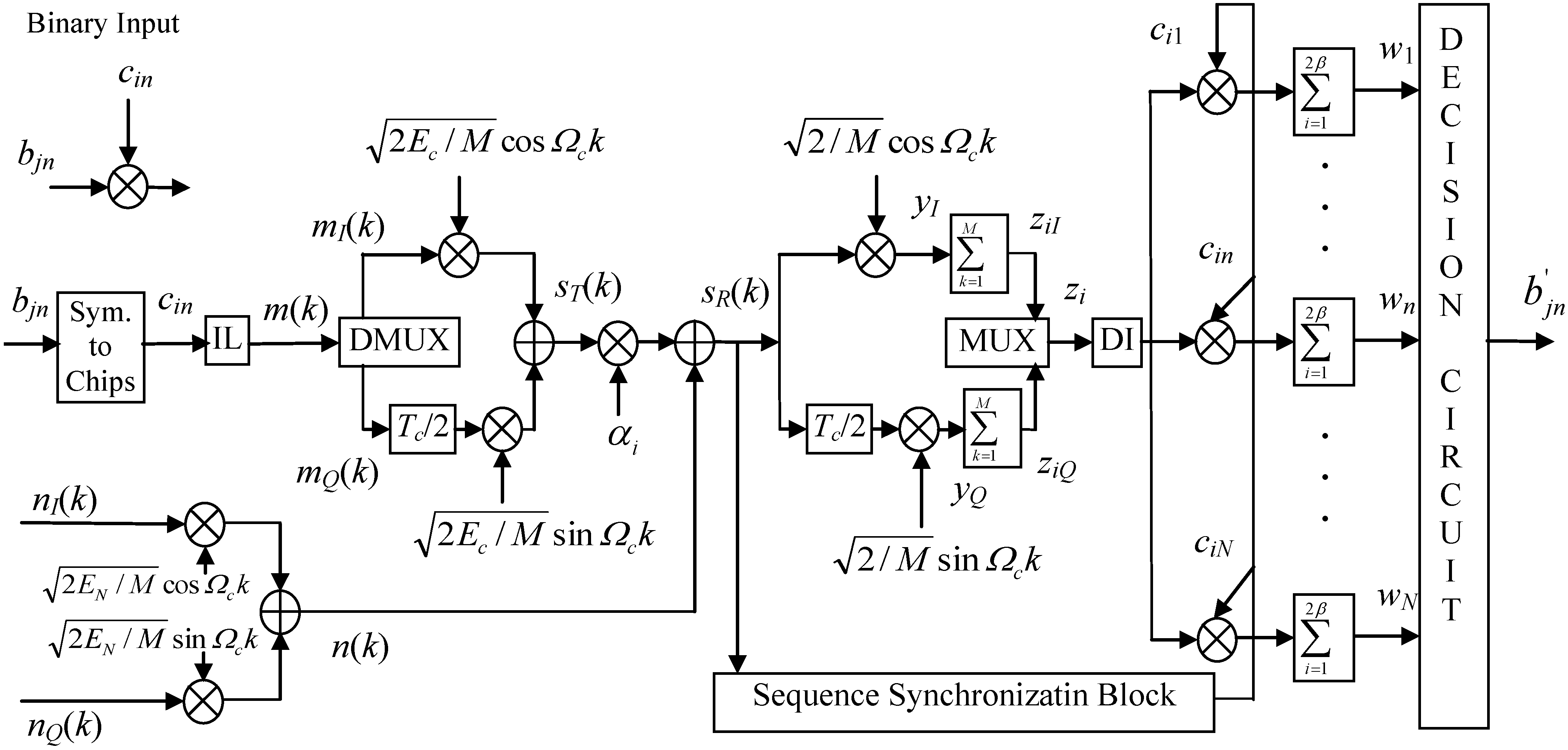
2.1. Single-Correlator Receiver
 and odd-indexed chip sequence mQ(k) modulates the quadrature carrier
  , where Ec is the energy per chip and M is the number of interpolated samples contained in one chip interval. Therefore, the transmitted signal can be defined as


 represents random variability of the spreading sequence. The energy of the noise is equivalent to the power spectral density of the two sided noise spectrum. As it was said before, this system is analyzed assuming that the signals are generated in discrete time domain. Each chip and related noise sample are generated once for each chip interval and then repeated (interpolated) M times in that chip interval to allow the discrete time carrier modulation. For M repeated samples of noise in a chip interval the energy is EN = Mσ2. For variance σ2 = BN0 and the bandwidth B=1/2Tc=1/2M, the energy is calculated to be EN = N0/2. If the source generates binary bits and the spreading sequence is in binary form, we may have
2.2. N-Correlator Receiver


3. Communication System Analysis in the Presence of Fading
3.1. Single-Correlator Receiver


 is the average signal-to-noise ratio defined as

3.2. N-Correlator Receiver


4. Interleaver Communication System Analysis in the Presence of Fading
4.1. Single Correlator Receiver


4.2. N-Correlator Receiver


5. Simulation Results and Discussions
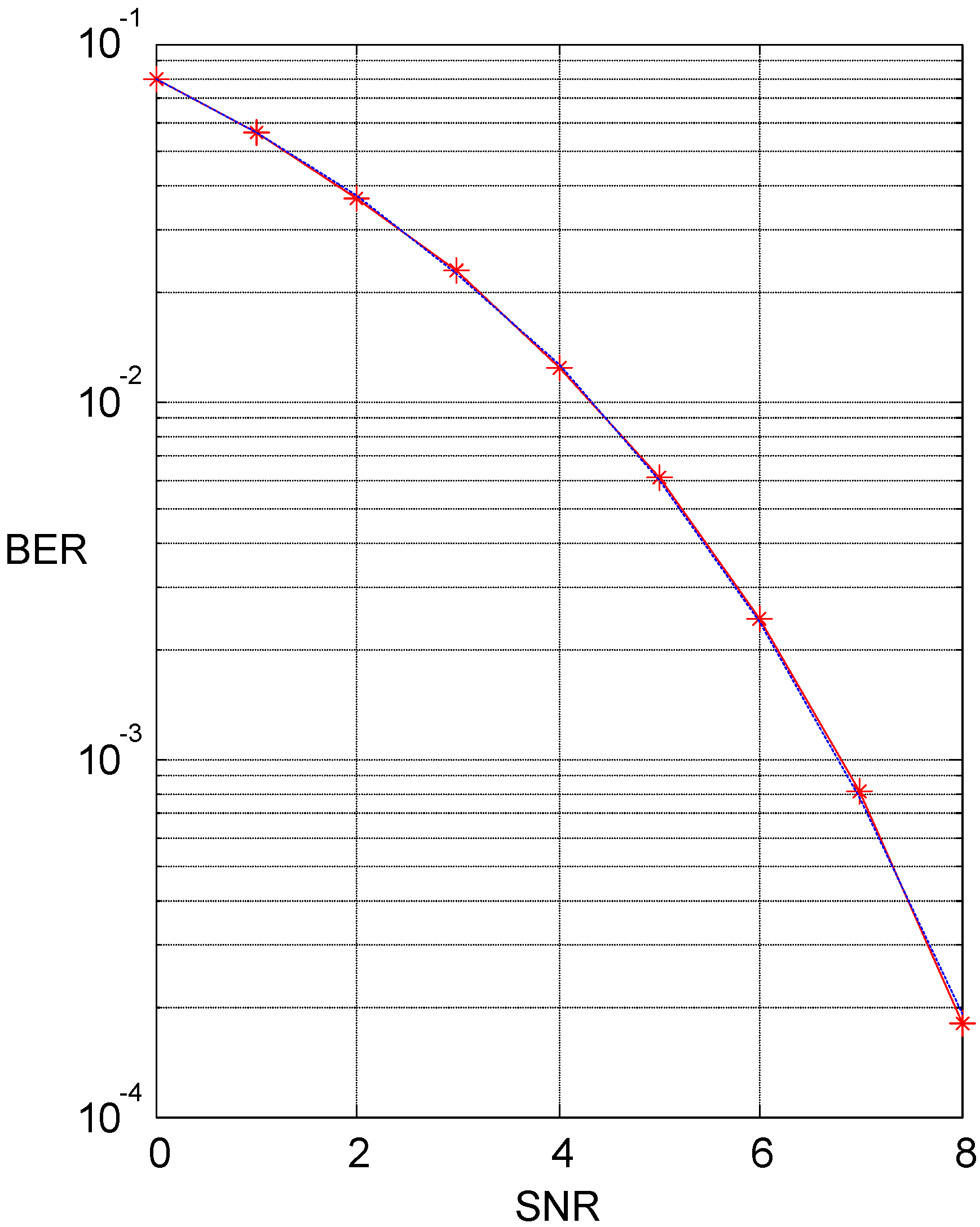
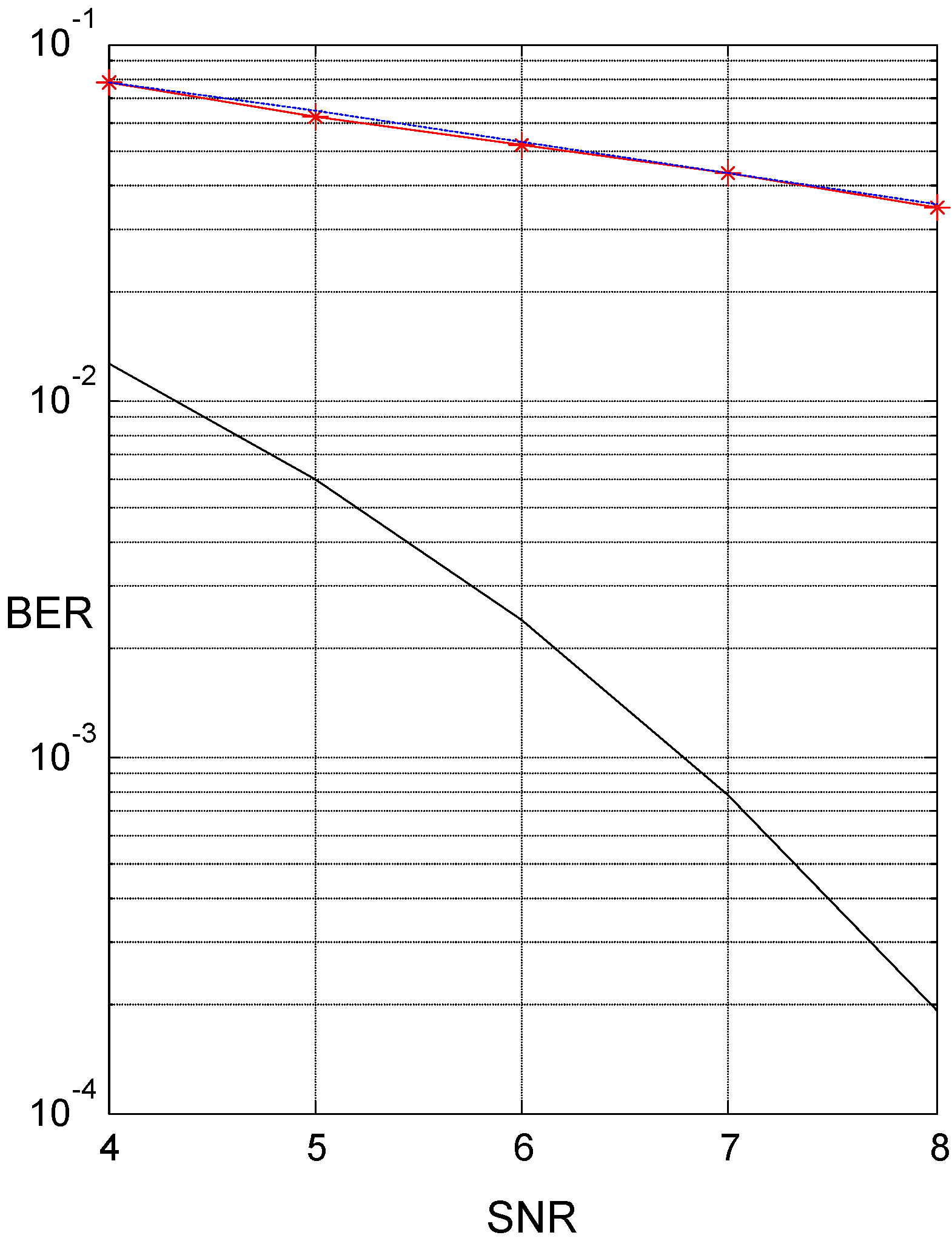
5.1. Single-Correlator Receiver


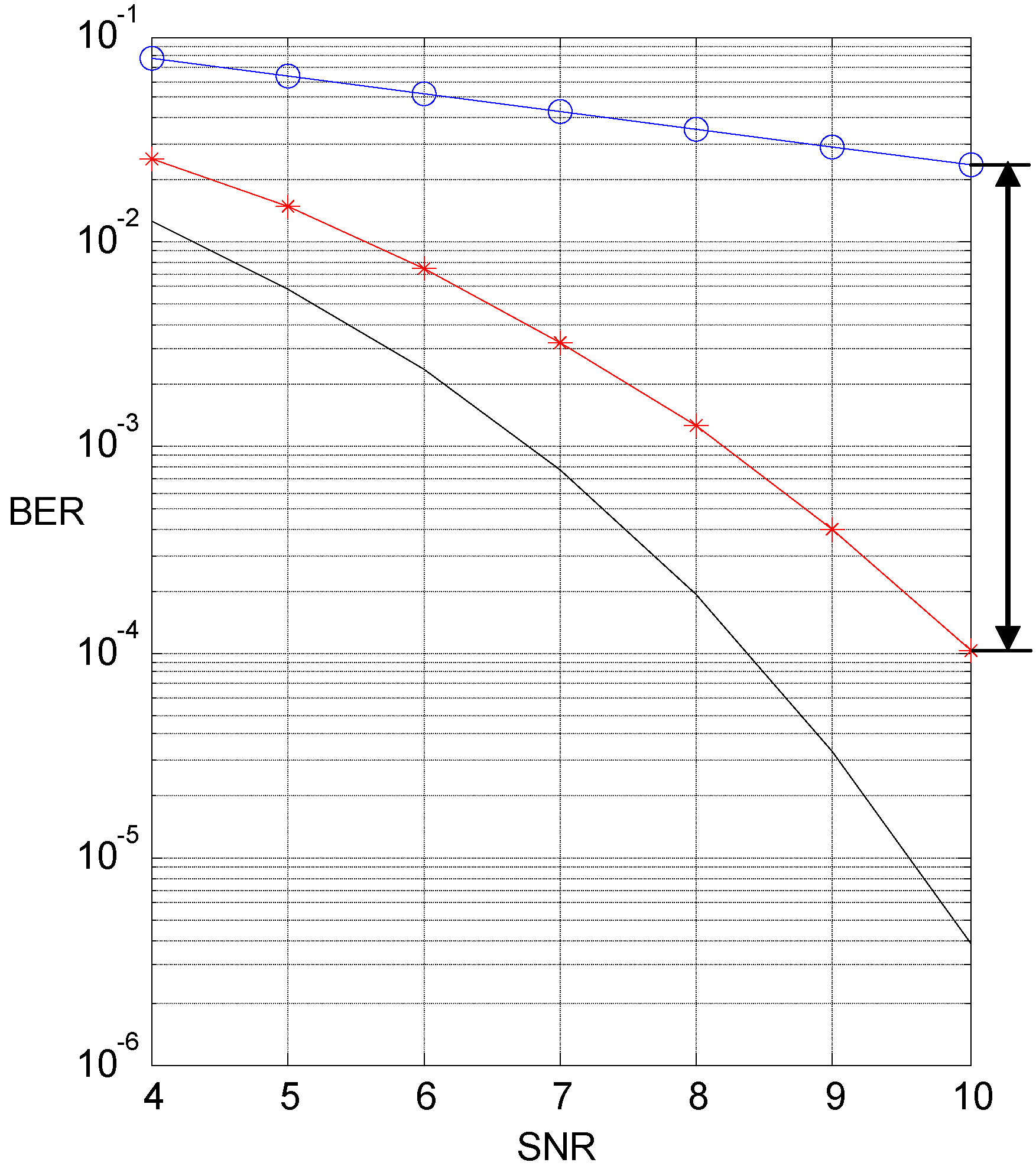
5.2. N-Correlator Receiver


6. Conclusions
Conflict of Interest
References
- IEEE Standard for Local and Metropolitan Area Networks—Part 15.4: Low-Rate Wireless Personal Area Networks (LR-WPANs); IEEE Standard 802.15.4–2011(Revision of IEEE Std 802.15.4–2006); IEEE: New York, NY, USA, 2011; pp. 1–294.
- Wang, C.C.; Huang, C.C.; Huang, J.M.; Chang, C.Y.; Li, C.P. Zig-Bee 868/915-MHz modulator/demodulator for wireless personal area network. IEEE Trans. Very-Large Scale Integr. (VLSI) Syst. 2008, 16, 936–938. [Google Scholar] [CrossRef]
- Oh, N.-J.; Lee, S.-G. Building 2.4-GHZ radio transceiver using IEEE 802.15.4. IEEE Circuits Devices Mag. 2006, 21, 43–51. [Google Scholar]
- Khalil, I.M.; Gadallah, Y.; Hayajneh, M.; Khreishah, A. An adaptive OFDMA-based MAC protocol for underwater acoustic wireless sensor networks. J. Sens. Actuat. Netw. 2012, 12, 8782–8805. [Google Scholar]
- Islam, M.R.; Han, Y.S. Cooperative MIMO communication at wireless sensor network: An error correcting code approach. J. Sens. Actuator Netw. 2011, 11, 9887–9903. [Google Scholar]
- Colistra, G.; Atzori, L. Estimation of physical layer performance in WSNs exploiting the method of indirect observations. J. Sens. Actuator Netw. 2012, 1, 272–298. [Google Scholar] [CrossRef]
- Gui, X. Chip-interleaving direct sequence spread spectrum system over Rician multipath fading channels. Wirel. Commun. Mob. Comput. 2011. [Google Scholar] [CrossRef]
- Mahadevappa, R.H.; Proakis, J.G. Mitigating multiple access interference and intersymbol interference in uncoded CDMA systems with chip-level interleaving. IEEE Trans. Wirel. Commun. 2002, 1, 781–792. [Google Scholar] [CrossRef]
- Berber, S.M.; Vali, R. Fading Mitigation in Interleaved Chaos-Based DS-CDMA Systems for Secure Communications. In Proceedings of the 15th World Scientific and Engineering Academy and Society (WSEAS) International Conference on Communications, Corfu, Greece, 15–17 July 2011; pp. 1–6.
- Lin, Y.-N.; Lin, D.W. Novel analytical results on performance of bit-interleaved and chip-interleaved DS-CDMA with convolutional coding. IEEE Trans. Veh. Technol. 2005, 54, 996–1012. [Google Scholar] [CrossRef]
- Vali, R.; Berber, M.S.; Nguang, K.S. Accurate derivation of chaos-based acquisition phase performance in a fading channel. IEEE Trans. Wirel. Commun. 2012, 11, 722–731. [Google Scholar] [CrossRef]
- Vali, R.; Berber, M.S.; Nguang, K.S. Analysis of chaos-based code tracking using chaotic correlation statistics. IEEE Trans. Circuits Syst.-I 2012, 59, 796–805. [Google Scholar] [CrossRef]
- Proakis, J.G. Digital Communications, 4th ed.; McGraw-Hill: New York, NY, USA, 2001. [Google Scholar]
- Berber, S.M. Bit error rate measurement with predetermined confidence. Inst. Electr. Eng. 1991, 27, 1205–1206. [Google Scholar]
- Berber, S.M.; Yuan, Y.; Suh, B. Derivation of BER Expressions and Simulation of a Chip Interleaved System for WSNs Application. In Proceedings of the 17th WSEAS International Conference on Communications, Rhodos, Greece, 16–19 July 2013; pp. 128–133.
© 2013 by the authors; licensee MDPI, Basel, Switzerland. This article is an open access article distributed under the terms and conditions of the Creative Commons Attribution license (http://creativecommons.org/licenses/by/3.0/).
Share and Cite
Berber, S.; Chen, N. Physical Layer Design in Wireless Sensor Networks for Fading Mitigation. J. Sens. Actuator Netw. 2013, 2, 614-630. https://doi.org/10.3390/jsan2030614
Berber S, Chen N. Physical Layer Design in Wireless Sensor Networks for Fading Mitigation. Journal of Sensor and Actuator Networks. 2013; 2(3):614-630. https://doi.org/10.3390/jsan2030614
Chicago/Turabian StyleBerber, Stevan, and Nuo Chen. 2013. "Physical Layer Design in Wireless Sensor Networks for Fading Mitigation" Journal of Sensor and Actuator Networks 2, no. 3: 614-630. https://doi.org/10.3390/jsan2030614
APA StyleBerber, S., & Chen, N. (2013). Physical Layer Design in Wireless Sensor Networks for Fading Mitigation. Journal of Sensor and Actuator Networks, 2(3), 614-630. https://doi.org/10.3390/jsan2030614