A Joint Routing and Channel Assignment Scheme for Hybrid Wireless-Optical Broadband-Access Networks †


Abstract
1. Introduction
- First, we develop a novel route quality metric that utilizes performance characteristics of data packet transmissions, and effectively captures the effects of intraflow and interflow interference.
- Second, we propose a joint routing and channel assignment protocol (JRCA) that tries to maximize the overall quality of communication paths in the network by employing the developed route quality metric. For channel assignment, JRCA employs a combination of backtracking and genetic algorithm to reduce the convergence time. The distinctive aspect of this work is that the WOBAN architecture enables the gateways to collaborate with each other through the optical backbone for determining the optimum gateway and route selections for all active nodes in the network. This allows for a hybrid design approach, i.e., combination of centralized and distributed, which is distinct from those followed in (purely) wireless mesh networks.
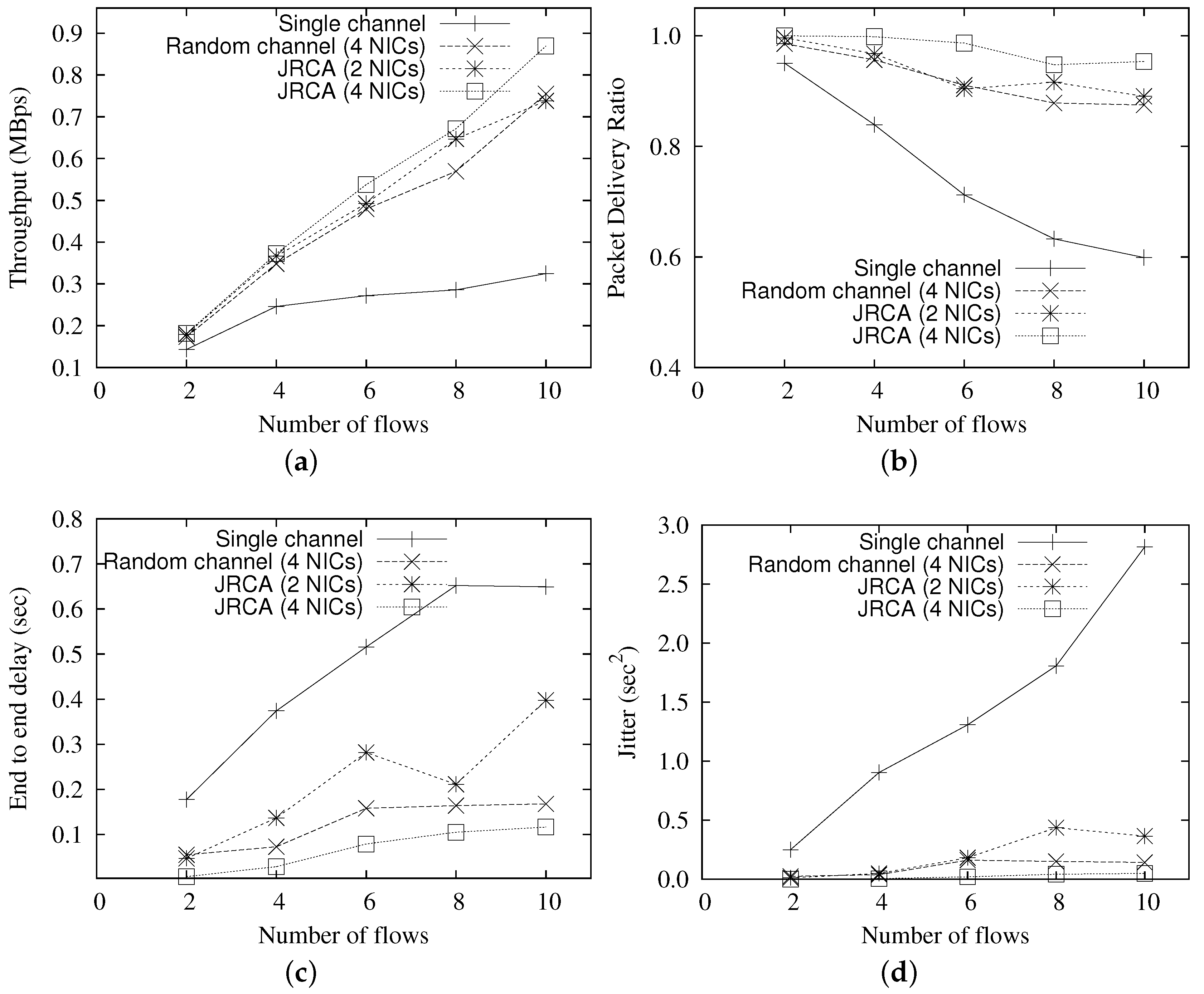
- Finally, we evaluate the performance of JRCA using extensive simulations. Performance evaluations show that, compared to a single channel scenario, JRCA improves the network throughput by up to three times, whereas reduces the traffic delay by ∼six times, with 12 orthogonal channels and four NICs per router.
2. System Overview and Research Directions in WOBAN
2.1. Current Trends in Access Networks
2.2. WOBAN Architecture and the Motivation behind WOBAN
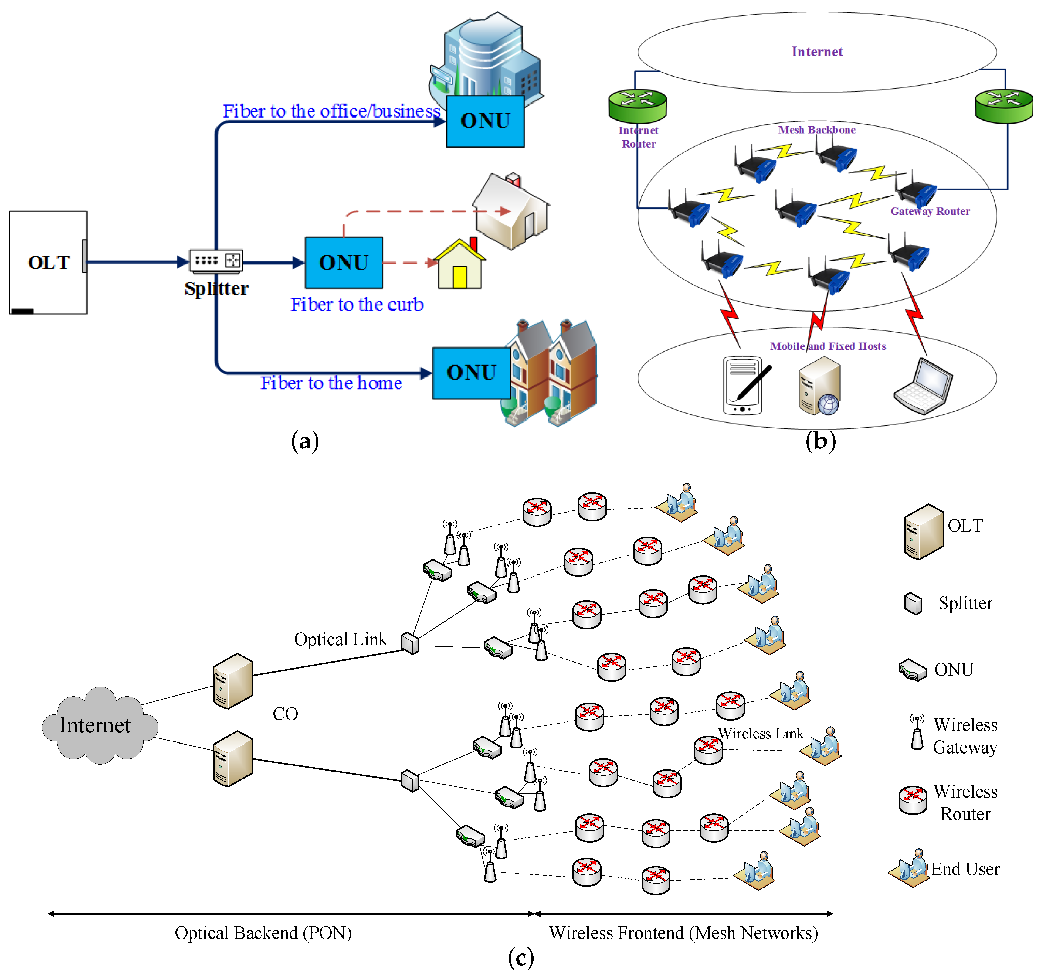
- A WOBAN can be more cost efficient as compared to a PON, since fibers in a WOBAN do not need to be penetrated to every subscriber’s homes, premises or offices. One estimate [4] shows that the cost to wire 80% of the US households with broadband lies between $60–120 billion, whereas using wireless drastically reduces the cost to $2 billion. Even in developing regions, the cost of providing and maintaining wireline broadband connectivity is prohibitively expensive. WOBAN-like hybrid architecture is particularly appealing in these scenarios where fiber layout is only needed from central offices to some ONU points, beyond which the wireless frontend consists of mesh routers that can be flexibly deployed.
- The wireless mesh architecture provides more flexible wireless access to users compared to optical access networks. It is often difficult to deploy optical fibers and equipments in highly populated areas as well as in rugged environments. In these environments, the wireless front-end can provide easy coverage and connectivity in a cost-effective manner. Hybrid optical-wireless networks, if properly designed, can achieve better deployment flexibility than traditional PON.
- The self-healing nature of the wireless front end makes WOBAN more robust and fault tolerant than traditional PON. In traditional PON, a fiber cut between the splitter and an ONU or between the splitter and the OLT makes some or all of the ONUs disconnected from OLT. In WOBAN, the traffic disrupted by any failure or fiber cut can still be forwarded through the mesh routers using multi-hop routing to other ONUs and then to the OLT.
- WOBAN enjoys the advantages of anycast routing [5,6]. If a gateway is congested, a wireless router can route its traffic through other gateways. This reduces load and congestion on that gateway and gives WOBAN a better load-balancing capability. Such schemes require information exchanges among the gateway nodes which is a key feature of a WOBAN, as they are connected through optical fibers but is absent in a pure wireless mesh network.
- WOBAN has much higher bandwidth capacity compared to the low capacity wireless networks, which reduces the traffic congestion, packet loss rate as well as end-to-end packet delay. For example, in Figure 1b, multiple mesh routers in the mesh backbone result in traffic congestion, wireless interference, and channel contention, which can be improved using multi-channel communication. However, even in case of multi-channel communication, interference is a limiting factor, which can be alleviated by collaboratively using the optical and wireless technologies.
- The distinctive aspect of the WOBAN architecture is that it enables the gateways to collaborate with each other through the optical backbone for determining the routing and load-balancing decisions based on the varying network traffic. This allows for a hybrid design approach, i.e., combination of centralized and distributed, which provides better flexibility and fault tolerance ability than those followed in (purely) wireless mesh networks.
2.3. Related Works
2.4. Challenges Addressed
3. A Quality Aware Routing Metric for WOBAN
3.1. Transmission Delay
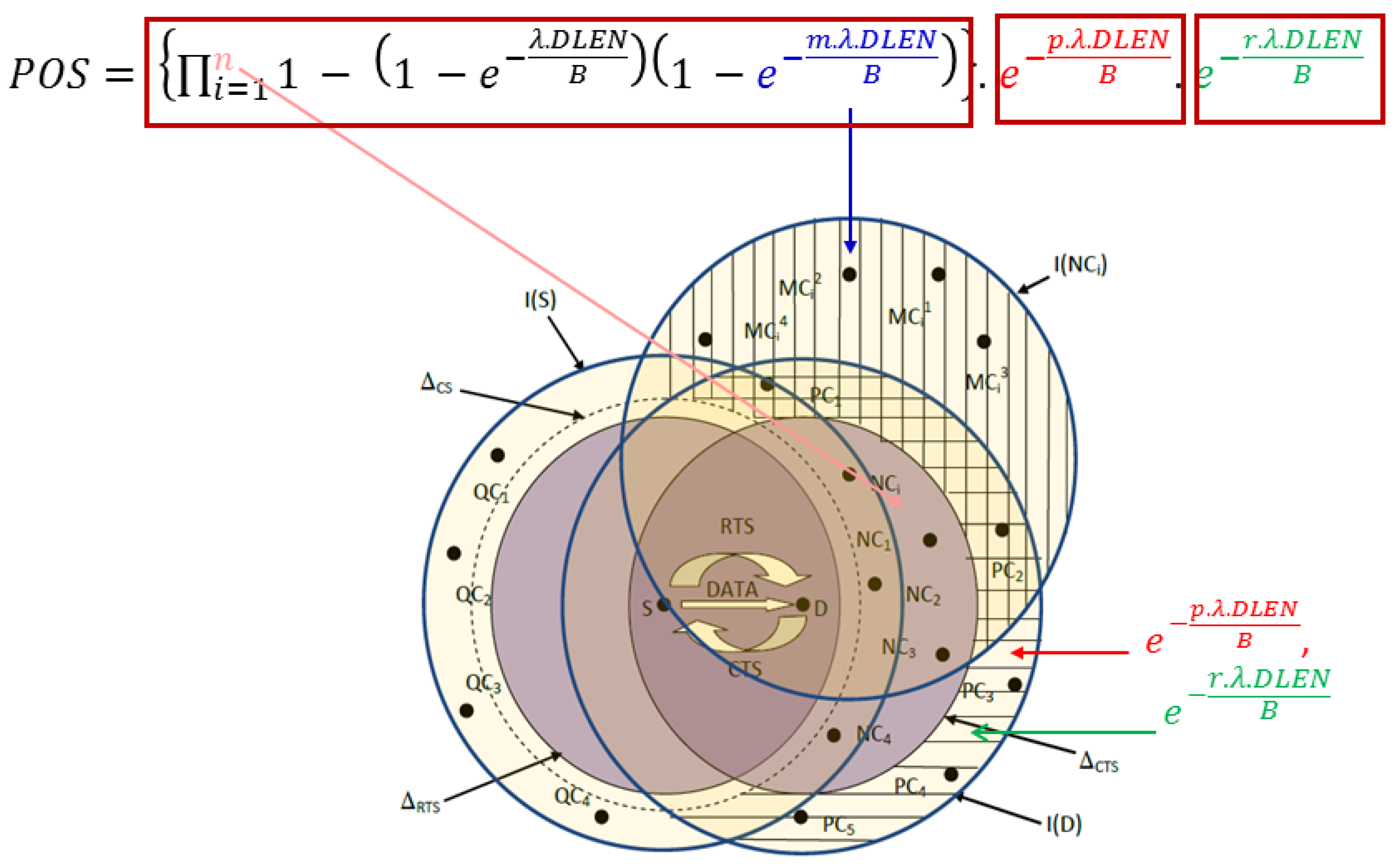
3.2. Probability of Success
4. Quality-Aware Routing and Channel Assignment in Multi-Channel Multi-Gateway WOBAN
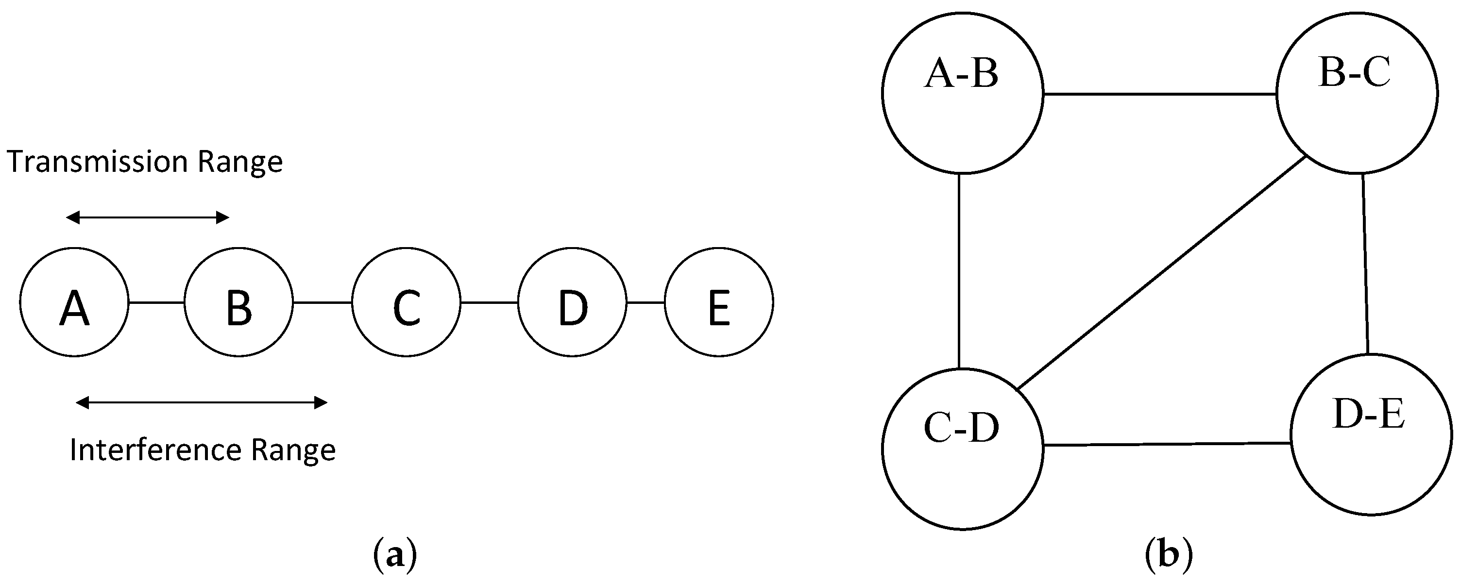
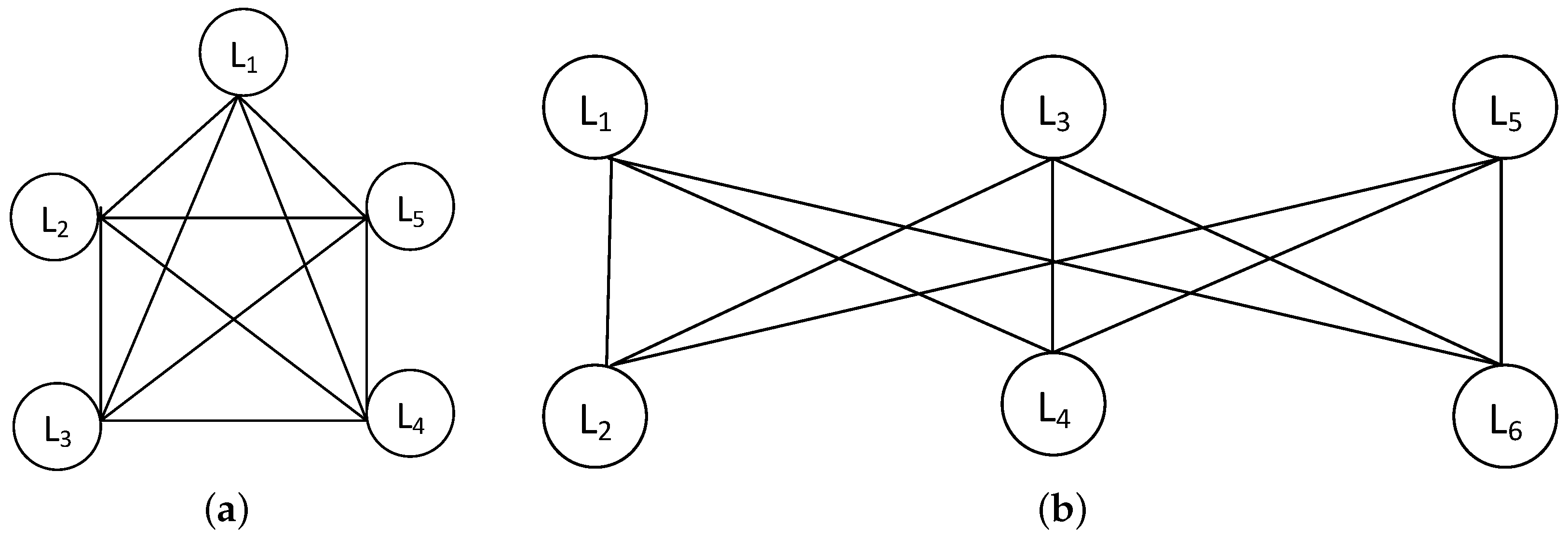
4.1. Conflict Graph and Planar Graph
4.2. Generating the Planar Subgraph of the Conflict Graph
| Algorithm 1 Function Vertex Deletion (Input graph G). | ||
| 1: | GCL = FCL = NULL; | |
| 2: | Sort ∈ G in decreasing order of vertex degree; | |
| 3: | while G ≠ PLANAR do | |
| 4: | G = G\, is of maximum degree in G; | ▹ Vertex with highest degree is removed from G |
| 5: | GCL = GCL ∪ ; | ▹ And placed in GCL |
| 6: | end while | |
| 7: | FCL = G; | ▹ Vertices of the planar graph G is stored in FCL |
| 8: | return GCL and FCL; | |
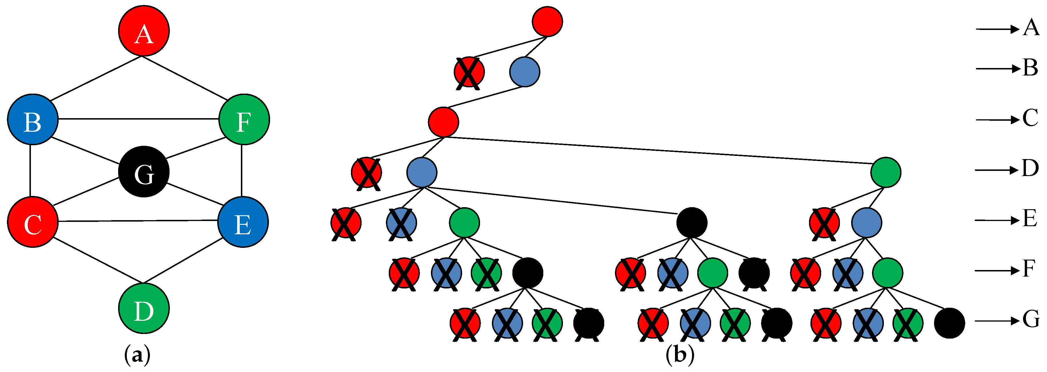
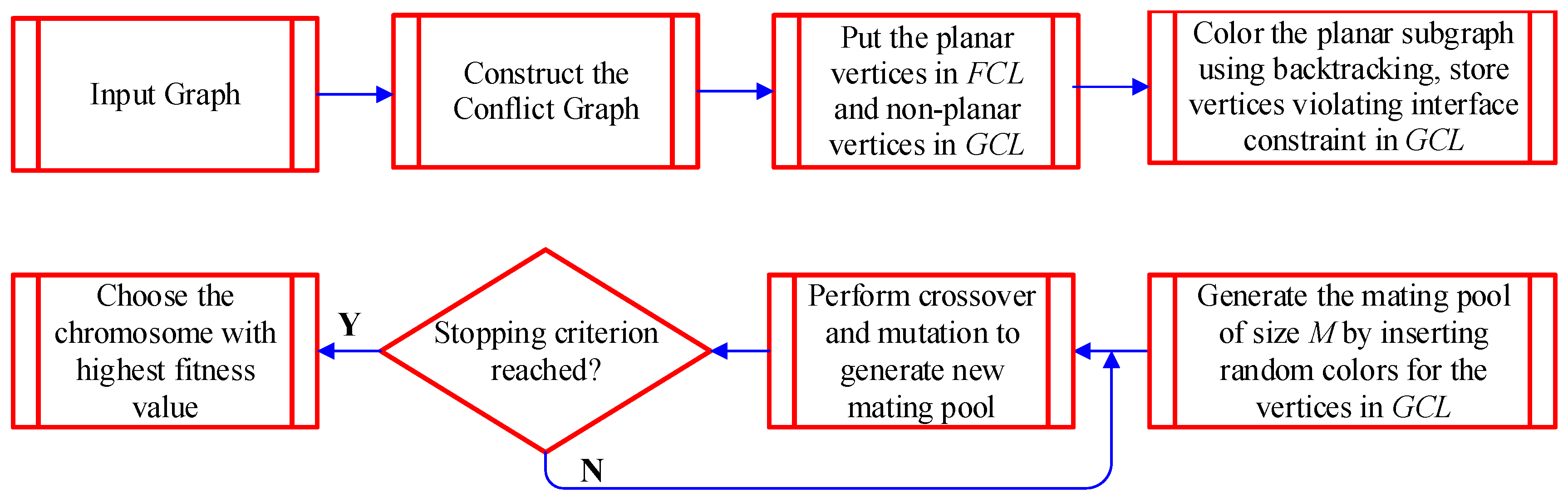
4.3. Our Proposed Algorithm for Coloring the Planar Subgraph
| Algorithm 2 Algorithm for finding the color/channel assignment. | |||
| 1: | INPUT: Simple undirected graph G and the set of channels; | ||
| 2: | OUTPUT: Color assignment of G; | ||
| 3: | Vertex Deletion (G); | ▹ To obtain the planar subgraph | |
| 4: | All_nodes_colored = false; | ||
| 5: | = ; | ||
| 6: | Color() = 0; | ||
| 7: | while All_nodes_colored == false do | ||
| 8: | while Color() < 4 do | ||
| 9: | if All_nodes_colored == true then | ||
| 10: | break; | ||
| 11: | end if | ||
| 12: | Color() = Color() + 1; | ▹ Color all vertices in G with at most 4 colors | |
| 13: | if ValidColor(Color(), ) == true then | ||
| 14: | if == then | ||
| 15: | All_nodes_colored = true; | ||
| 16: | else | ||
| 17: | = ; | ||
| 18: | Color() = 0; | ||
| 19: | end if | ||
| 20: | end if | ||
| 21: | end while | ||
| 22: | = ; | ▹ Backtrack if the vertex cannot be colored with 4 colors | |
| 23: | end while | ||
| 24: | GCL = GCL ∪ (vertices violating interface-constraint); | ▹ Vertices violating the interface-constraint are added to the GCL | |
| 25: | Perform Genetic-Algorithm(GCL); | ||
| 26: | return G with vertex coloring; | ||
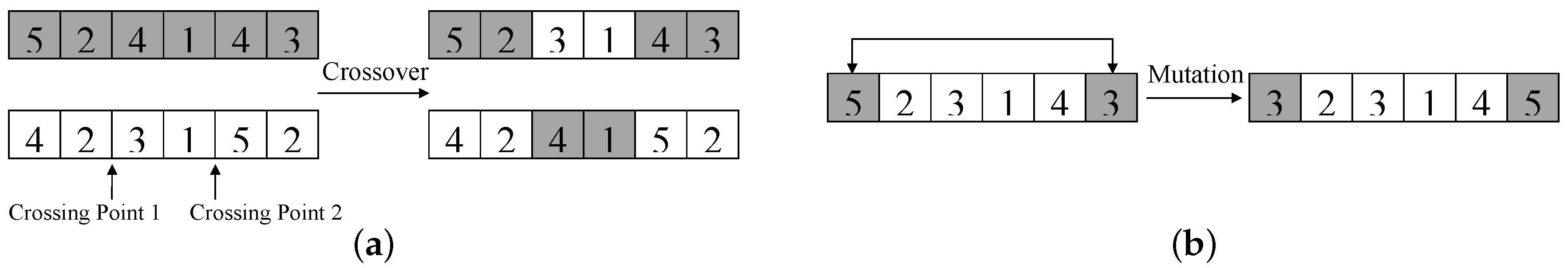
4.4. Our Proposed Genetic Algorithm for Channel Selection
4.5. Complexity of the Proposed Channel Assignment Scheme
4.6. JRCA Routing Protocol
5. Performance Evaluation of Our Routing Protocol
5.1. Comparison with Different Number of Flows
5.2. Comparison with Different Loads
5.3. Comparison with Different Number of Channels
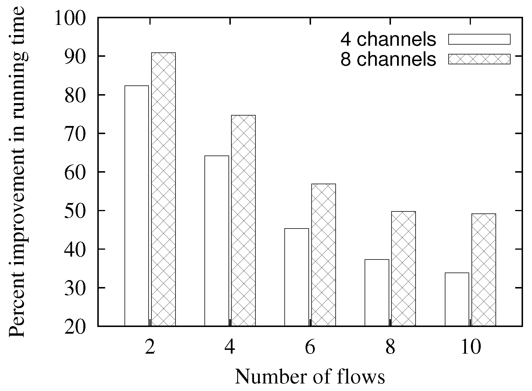
5.4. Comparison of Running Time
6. Conclusions
Author Contributions
Funding
Conflicts of Interest
Abbreviations
| WOBAN | Wireless-Optical Broadband-Access Networks |
| ONU | Optical Network Unit |
| OLT | Optical Line Terminal |
| CO | Central Office |
| PON | Passive Optical Network |
| EPON | Ethernet Passive Optical Network |
| GPON | Gigabit Passive Optical Network |
| BPON | Broadband Passive Optical Network |
| TDMA | Time-Division Multiple Access |
| WDM-PON | Wavelength Division Multiplexing-Passive Optical Network |
| WiFi | Wireless Fidelity |
| WiMAX | Worldwide Interoperability for Microwave Access |
| WMAN | Wireless Metropolitan-Area Networks |
| RoF | Radio-over-fiber |
| NICs | Network Interface Cards |
| MAC | Medium Access Control |
| DCF | Distributed Coordination Function |
| SINR | Signal-to-interference-plus-noise ratio |
| POS | Probability of Success |
| RTS/CTS | Request to Send/Clear to Send |
| ACK | Acknowledgement |
| CSMA/CA | Carrier-Sense Multiple Access with Collision Avoidance |
| UDP | User Datagram Protocol |
| JRCA | Joint Routing and Channel Assignment |
References
- Global Internet Users and Penetration Rate. Available online: https://www.electronicdesign.com/communications/these-technologies-will-bring-gigabit-home (accessed on 12 October 2018).
- Pal, A.; Nasipuri, A. JRCA: A Joint Routing and Channel Assignment Scheme for Wireless Mesh Networks. In Proceedings of the IEEE International Performance Computing and Communications Conference (2011), Orlando, FL, USA, 17–19 November 2011. [Google Scholar]
- Wireless Networking: Understanding Various Wireless LAN Technologies. Available online: https://thecybersecurityman.com/2018/08/30/wireless-networking-understanding-various-wireless-lan-technologies/ (accessed on 12 October 2018).
- Sarkar, S.; Dixit, S.; Mukherjee, B. Hybrid Wireless-Optical Broadband-Access Network (WOBAN): A Review of Relevant Challenges. J. Lightw. Technol. 2007, 25, 3329–3340. [Google Scholar] [CrossRef]
- Pal, A.; Nasipuri, A. A Quality Aware Anycast Routing Protocol for Wireless Mesh Networks. In Proceedings of the IEEE SoutheastCon, Concord, NC, USA, 18–21 March 2010; pp. 451–454. [Google Scholar]
- Pal, A.; Nasipuri, A. GSQAR: A Quality Aware Anycast Routing Protocol for Wireless Mesh Networks. In Proceedings of the IEEE Global Telecommunications Conference GLOBECOM, Miami, FL, USA, 6–10 December 2010. [Google Scholar]
- Song, L.; Zheng, B. An Anycast Routing Protocol for Wireless Mesh Access Network. In Proceedings of the 2009 WASE International Conference on Information Engineering, Taiyuan, China, 10–11 July 2009; Volume 2, pp. 82–85. [Google Scholar] [CrossRef]
- Sharif, K.; Cao, L.; Wang, Y.; Dahlberg, T.A. A Hybrid Anycast Routing Protocol for Load Balancing in Heterogeneous Access Networks. In Proceedings of the 17th International Conference on Computer Communications and Networks, St. Thomas, Virgin Islands, USA, 3–7 August 2008; pp. 99–104. [Google Scholar]
- Lakshmanan, S.; Sivakumar, R.; Sundaresan, K. Multi-gateway association in wireless mesh networks. Ad Hoc Netw. 2009, 7, 622–637. [Google Scholar] [CrossRef]
- Nandiraju, D.; Santhanam, L.; Nandiraju, N.; Agrawal, D. Achieving Load Balancing in Wireless Mesh Networks Through Multiple Gateways. In Proceedings of the IEEE International Conference on Mobile Adhoc and Sensor Systems Conference (2006), Vancouver, BC, Canada, 9–12 October 2006; pp. 807–812. [Google Scholar]
- Marina, M.K.; Das, S.R. A topology control approach for utilizing multiple channels in multi-radio wireless mesh networks. In Proceedings of the International Conference on Broadband Networks, Boston, MA, USA, 7 October 2005; pp. 412–421. [Google Scholar]
- Subramanian, A.P.; Gupta, H.; Das, S.R.; Cao, J. Minimum Interference Channel Assignment in Multiradio Wireless Mesh Networks. IEEE Trans. Mob. Comput. 2008, 7, 1459–1473. [Google Scholar] [CrossRef]
- Das, A.K.; Vijayakumar, R.; Roy, S. Static Channel Assignment in Multi-radio Multi-Channel 802.11 Wireless Mesh Networks: Issues, Metrics and Algorithms. In Proceedings of the IEEE Global Telecommunications Conference GLOBECOM, San Francisco, CA, USA, 27 November–1 December 2006; pp. 1–6. [Google Scholar]
- Das, A.K.; Alazemi, H.M.K.; Vijayakumar, R.; Roy, S. Optimization models for fixed channel assignment in wireless mesh networks with multiple radios. In Proceedings of the Second Annual IEEE Communications Society Conference on Sensor and Ad Hoc Communications and Networks, Santa Clara, CA, USA, 26–29 September 2005; pp. 463–474. [Google Scholar]
- Kodialam, M.; Nandagopal, T. Characterizing the capacity region in multi-radio multi-channel wireless mesh networks. In Proceedings of the 11th Annual International Conference on Mobile Computing and Networking, Cologne, Germany, 28 August–2 September 2005; ACM Press: New York, NY, USA, 2005; pp. 73–87. [Google Scholar]
- Koshy, R.; Ruan, L. A Joint Radio and Channel Assignment (JRCA) Scheme for 802.11-Based Wireless Mesh Networks. In Proceedings of the 2009 IEEE Globecom Workshops, Honolulu, HI, USA, 30 November–4 December 2009. [Google Scholar]
- Raniwala, A.; Gopalan, K.; Cker Chiueh, T. Centralized Channel Assignment and Routing Algorithms for Multi-channel Wireless Mesh Networks. ACM Mob. Comput. Commun. Rev. 2004, 8, 50–65. [Google Scholar] [CrossRef]
- Raniwala, A.; Cker Chiueh, T. Architecture and algorithms for an IEEE 802.11-based multi-channel wireless mesh network. In Proceedings of the 24th Annual Joint Conference of the IEEE Computer and Communications Societies, Miami, FL, USA, 13–17 March 2005; pp. 2223–2234. [Google Scholar]
- Chen, J.; Jia, J.; Wen, Y.; Zhao, D.; Liu, J. A genetic approach to channel assignment for multi-radio multi-channel wireless mesh networks. In Proceedings of the ACM/SIGEVO Summit on Genetic and Evolutionary Computation, Shanghai, China, 12–14 June 2009; pp. 39–46. [Google Scholar]
- Fu, W.; Xie, B.; Wang, X.; Agrawal, D.P. Flow-Based Channel Assignment in Channel Constrained Wireless Mesh Networks. In Proceedings of the 17th International Conference on Computer Communications and Networks, St. Thomas, Virgin Islands, USA, 3–7 August 2008; pp. 424–429. [Google Scholar]
- Kyasanur, P.; Vaidya, N.H. Routing and link-layer protocols for multi-channel multi-interface ad hoc wireless networks. SIGMOBILE Mob. Comput. Commun. Rev. 2006, 10, 31–43. [Google Scholar] [CrossRef]
- Ramachandran, K.N.; Belding, E.M.; Almeroth, K.C.; Buddhikot, M.M. Interference-Aware Channel Assignment in Multi-Radio Wireless Mesh Networks. In Proceedings of the 25th IEEE International Conference on Computer Communications, Barcelona, Spain, 23–29 April 2006; pp. 1–12. [Google Scholar]
- Li, Y.; Wang, J.; Qiao, C.; Gumaste, A.; Xu, Y.; Xu, Y. Integrated Fiber-Wireless (FiWi) Access Networks Supporting Inter-ONU Communications. J. Lightw. Technol. 2010, 28, 714–724. [Google Scholar]
- Shaw, W.T.; Wong, S.W.; Cheng, N.; Kazovsky, L. MARIN Hybrid Optical-Wireless Access Network. In Proceedings of the Optical Fiber Communication Conference and Exposition and The National Fiber Optic Engineers Conference, Anaheim, CA, USA, 25–29 March 2007. [Google Scholar]
- Wong, S.-W.; Campelo, D.R.; Cheng, N.; Yen, S.-H.; Kazovsky, L.; Lee, H.; Cox, D.C. Grid Reconfigurable Optical-Wireless Architecture for Large Scale Municipal Mesh Access Network. In Proceedings of the IEEE Global Telecommunications Conference, Honolulu, HI, USA, 30 Novomber–4 December 2009. [Google Scholar]
- Kanonakis, K.; Tomkos, I.; Pfeiffer, T.; Prat, J.; Kourtessis, P. ACCORDANCE: A novel OFDMA-PON paradigm for ultra-high capacity converged wireline-wireless access networks. In Proceedings of the International Conference on Transparent Optical Networks, Munich, Germany, 27 June–1 July 2010. [Google Scholar]
- Kazovsky, L.; Wong, S.; Ayhan, T.; Albeyoglu, K.M.; Ribeiro, M.R.N.; Shastri, A. Hybrid Optical-Wireless Access Networks. Proc. IEEE 2012, 100, 1197–1225. [Google Scholar] [CrossRef]
- Sarigiannidis, A.; Iloridou, M.; Nicopolitidis, P.; Papadimitriou, G.I.; Pavlidou, F.; Sarigiannidis, P.G.; Louta, M.D.; Vitsas, V. Architectures and Bandwidth Allocation Schemes for Hybrid Wireless-Optical Networks. IEEE Commun. Surv. Tutor. 2015, 17, 427–468. [Google Scholar] [CrossRef]
- Sarkar, S.; Mukherjee, B.; Dixit, S. Optimum Placement of Multiple Optical Network Units (ONUs) in Optical-Wireless Hybrid Access Networks. In Proceedings of the Optical Fiber Communication Conference and Exposition and The National Fiber Optic Engineers Conference, Anaheim, CA, USA, 5–10 March 2006. [Google Scholar]
- Sarkar, S.; Mukherjee, B.; Dixit, S. Towards global optimization of multiple ONUs placement in hybrid optical-wireless broadband access networks. In Proceedings of the Joint International Conference on Optical Internet and Next Generation Network, Jeju, Korea, 9–13 July 2006; pp. 65–67. [Google Scholar]
- Sarkar, S.; Mukherjee, B.; Dixit, S. A mixed integer programming model for optimum placement of base stations and optical network units in a hybrid wireless-optical broadband access network (WOBAN). In Proceedings of the Wireless Communications and Networking Conference, Hong Kong, China, 11–15 March 2007. [Google Scholar]
- Sarkar, S.; Yen, H.; Dixit, S.S.; Mukherjee, B. A novel delay-aware routing algorithm (DARA) for a hybrid wireless-optical broadband access network (WOBAN). IEEE Netw. 2008, 22, 20–28. [Google Scholar] [CrossRef]
- Reaz, A.A.S.; Ramamurthi, V.; Sarkar, S.; Ghosal, D.; Dixit, S.S.; Mukherjee, B. CaDAR: An Efficient Routing Algorithm for Wireless-Optical Broadband Access Network. In Proceedings of the IEEE International Conference on Communications, Beijing, China, 19–23 May 2008; pp. 5191–5195. [Google Scholar]
- Reaz, A.S.; Ramamurthi, V.; Tornatore, M.; Sarkar, S.; Ghosal, D.; Mukherjee, B. Cost-efficient design for higher capacity hybrid wireless-optical broadband access network (WOBAN). Comput. Netw. 2011, 55, 2138–2149. [Google Scholar] [CrossRef]
- Pal, A.; Nasipuri, A. Performance analysis of IEEE 802.11 distributed coordination function in presence of hidden stations under non-saturated conditions with infinite buffer in radio-over-fiber wireless LANs. In Proceedings of the IEEE Workshop on Local & Metropolitan Area Networks, Chapel Hill, NC, USA, 13–14 October 2011; pp. 1–6. [Google Scholar]
- Pal, A.; Adimadhyam, S.; Nasipuri, A. QoSBR: A Quality Based Routing Protocol for Wireless Mesh Networks. In Proceedings of the International Conference on Distributed Computing and Networking, Kolkata, India, 3–6 January 2011; pp. 497–508. [Google Scholar]
- Pal, A.; Nasipuri, A. A Quality Based Routing Protocol for Wireless Mesh Networks. Pervasive Mob. Comput. 2011, 7, 611–626. [Google Scholar] [CrossRef]
- Garey, M. Computers and Intractability—A Guide to the Theory of NP-Completeness; W. H. Freeman & Co.: New York, NY, USA, 1990. [Google Scholar]
- Genetic Algorithms. Available online: http://www.obitko.com/tutorials/genetic-algorithms/ (accessed on 12 October 2018).
- Jain, K.; Padhye, J.; Padmanabhan, V.N.; Qiu, L. Impact of interference on multi-hop wireless network performance. In Proceedings of the International Conference on Mobile Computing and Networking, San Diego, CA, USA, 14–19 September 2003; pp. 66–80. [Google Scholar]
- Cormen, T.H.; Leiserson, C.E.; Rivest, R.L.; Stein, C. Introduction to Algorithms, 3rd ed.; The MIT Press: Cambridge, MA, USA, 2009. [Google Scholar]
- Trudeau, R.J. Introduction to Graph Theory; Dover Books on Mathematics; Dover: Mineola, NY, USA, 1994. [Google Scholar]
- Appel, K.; Haken, W. Every planar map is four colorable. Part I: Discharging. Ill. J. Math. 1977, 21, 429–490. [Google Scholar]
- Boyer, J.M.; Myrvold, W.J. On the cutting edge: Simplified O(n) planarity by edge addition. J. Gr. Algorithms Appl. 2004, 8, 241–273. [Google Scholar] [CrossRef]
- Hubai, T. The Chromatic Polynomial. Master’s Thesis, Eötvös Loránd University, Budapest, Hungary, 2009. [Google Scholar]
- Faria, L.; de Figueiredo, C.M.H.; Gravier, S.; Mendonca, C.F.; Stolfi, J. Nonplanar vertex deletion: Maximum degree thresholds for NP/Max SNP-hardness and a -approximation for finding maximum planar induced subgraphs. Electron. Notes Discret. Math. 2004, 18, 121–126. [Google Scholar] [CrossRef]
- Louis, S.J.; Rawlins, G.J.E. Predicting Convergence Time for Genetic Algorithms. Found. Genet. Algorithms 1992, 2, 141–161. [Google Scholar]
- Wilf, S. Backtrack: an O(1) Expected Time Algorithm for the Graph Coloring Problem. Inf. Process. Lett. 1984, 18, 119–121. [Google Scholar] [CrossRef]
- The Netwrok Simulator ns-2. Available online: http://www.isi.edu/nsnam/ns/ (accessed on 12 October 2018).


| Standard | Frequency | Bandwidth | Non-Overlapping Channels |
|---|---|---|---|
| 802.11b | 2.4 GHz | 20 MHz | 3 non-overlapping channels (channels 1, 6, and 11) |
| 802.11a | 5 GHz | 20 MHz | 24 non-overlapping 20 MHz channels, and 12 non-overlapping 40 MHz channels |
| 802.11g | 2.4 GHz | 20 MHz | 3 non-overlapping channels (channels 1, 6, and 11) |
| 802.11n | 2.4/5 GHz | 20, 40 MHz | In 2.4 GHz band, there are 3 non-overlapping 20 MHz channels (channels 1, 6, and 11), and 1 non-overlapping 40 MHz channels (channel 3). In 5 GHz band, there are 24 non-overlapping 20 MHz channels, and 12 non-overlapping 40 MHz channels |
| 802.11ac | 5 GHz | 20, 60, 80, 160 MHz | 24 non-overlapping 20 MHz channels, 12 non-overlapping 40 MHz channels, 6 non-overlapping 80 MHz channels, and 2 non-overlapping 160 MHz channels |
| ≜ | Active neighbors of the sender/receiver | |
| ≜ | Transmission delay | |
| ≜ | Regions where the RTS/CTS packets for the test link are received | |
| ≜ | Area where nodes can sense the transmission from sender S | |
| ≜ | Packet arrival rate | |
| ≜ | Data packet length (in bits) | |
| B | ≜ | Channel bandwidth (in bits/seconds) |
| ≜ | Probability of success | |
| ≜ | Quality metric for route R | |
| ≜ | Complete bipartite graph with vertices and edges | |
| ≜ | Complete graph of n vertices | |
| C | ≜ | Number of channels |
| I | ≜ | Number of interfaces |
| ≜ | Planar subgraph of G | |
| M | ≜ | Number of chromosomes in the mating pool |
| ≜ | Number of elite chromosomes |
| Parameter | Values | Parameter | Values |
|---|---|---|---|
| Max queue length | 200 | Data packets size | 1000 bytes |
| Propagation Model | Two Ray Ground | Traffic Generation | Exponential |
| Antenna gain | 0 dB | Transmit power | 20 dBm |
| Noise floor | −101 dBm | SINRDatacapture | 10 dB |
| Bandwidth | 6 Mbps | PowerMonitor Thresh | −86.77 dBm |
| Average ON time | 0.5 s | Average OFF time | 0.5 s |
© 2018 by the authors. Licensee MDPI, Basel, Switzerland. This article is an open access article distributed under the terms and conditions of the Creative Commons Attribution (CC BY) license (http://creativecommons.org/licenses/by/4.0/).
Share and Cite
Pal, A.; Nasipuri, A. A Joint Routing and Channel Assignment Scheme for Hybrid Wireless-Optical Broadband-Access Networks. J. Sens. Actuator Netw. 2018, 7, 44. https://doi.org/10.3390/jsan7040044
Pal A, Nasipuri A. A Joint Routing and Channel Assignment Scheme for Hybrid Wireless-Optical Broadband-Access Networks. Journal of Sensor and Actuator Networks. 2018; 7(4):44. https://doi.org/10.3390/jsan7040044
Chicago/Turabian StylePal, Amitangshu, and Asis Nasipuri. 2018. "A Joint Routing and Channel Assignment Scheme for Hybrid Wireless-Optical Broadband-Access Networks" Journal of Sensor and Actuator Networks 7, no. 4: 44. https://doi.org/10.3390/jsan7040044
APA StylePal, A., & Nasipuri, A. (2018). A Joint Routing and Channel Assignment Scheme for Hybrid Wireless-Optical Broadband-Access Networks. Journal of Sensor and Actuator Networks, 7(4), 44. https://doi.org/10.3390/jsan7040044