Abstract
The Robotic Vessels as-a-Service (RoboVaaS) project intends to exploit the most advanced communication and marine vehicle technologies to revolutionize shipping and near-shore operations, offering on-demand and cost-effective robotic-aided services. In particular, the RoboVaaS vision includes a ship hull inspection service, a quay walls inspection service, an antigrounding service, and an environmental and bathymetry data collection service. In this paper, we present a study of the underwater environmental data collection service, performed by a low-cost autonomous vehicle equipped with both a commercial modem and a very low-cost acoustic modem prototype, the smartPORT Acoustic Underwater Modem (AHOI). The vehicle mules the data from a network of low cost submerged acoustic sensor nodes to a surface sink. To this end, an underwater acoustic network composed by both static and moving nodes has been implemented and simulated with the DESERT Underwater Framework, where the performance of the AHOI modem has been mapped in the form of lookup tables. The performance of the AHOI modem has been measured near the Port of Hamburg, where the RoboVaaS concept will be demonstrated with a real field evaluation. The transmission with the commercial modem, instead, has been simulated with the Bellhop ray tracer thanks to the World Ocean Simulation System (WOSS), by considering both the bathymetry and the sound speed profile of the Port of Hamburg. The set up of the polling-based MAC protocol parameters, such as the maximum backoff time of the sensor nodes, appears to be crucial for the network performance, in particular for the low-cost low-rate modems. In this work, to tune the maximum backoff time during the data collection mission, an adaptive mechanism has been implemented. Specifically, the maximum backoff time is updated based on the network density. This adaptive mechanism results in an 8% improvement of the network throughput.
1. Introduction
The Robotic Vessels as-a-Service (RoboVaaS) project intends to revolutionize shipping and near-shore operations, by exploiting the most advanced communication and marine vehicle technologies to offer on-demand robotic-aided services (Figure 1). Specifically, these services include ship-hull inspection, quay walls inspection, anti-grounding, and environmental and bathymetry data collection. In this paper, we address the study of the underwater environmental data collection service in the scenario of the port of Hamburg, characterized by shallow turbid fresh water, where the RoboVaaS concept will be demonstrated as part of the project. The environmental data is retrieved by an underwater sensor network (USN), that is typically employed to monitor the water quality and the water characteristics of oceans, rivers and lakes, in order to inspect the impact of human activities on the sea life, as well as to monitor the coastal erosion and perform tsunami prevention [1]. One of the most effective approaches to retrieve the data from these submerged sensors is to employ an autonomous underwater vehicle (AUV) [2] that patrols the area where the USN is deployed, and mules the data from the USN to a surface sink connected to shore (Figure 2). The sink can be either a surface buoy or an autonomous surface vessel (ASV). The main challenge of this application is the data transmission from the USN to the AUV, and from the AUV to the sink. Indeed the underwater scenario is, by its nature, very challenging for radio wireless communications, as electromagnetic waves are drastically attenuated. For this reason, they can only be used for very short range broadband links [3]. Similarly, also underwater optical communications are used only for very short range links, as they are affected by turbidity and solar noise. Usually, they are employed only in deep water scenarios, where the turbidity is typically very low and the surrounding light noise is negligible [4].
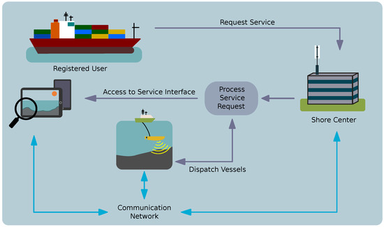
Figure 1.
Robotic Vessels-as-a-Service (RoboVaaS) envisioned example scenario showing ship-hull inspection and anti-grounding services enabled through a fleet of autonomous vessels connected with acoustic underwater and surface radio communication.
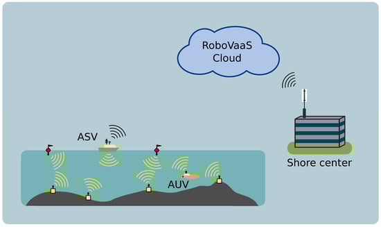
Figure 2.
RoboVaaS underwater data collection service, where both an autonomous surface vessel (ASV) and an autonomous underwater vehicle (AUV) collect data from static underwater sensor nodes. The figure also portrays the inclusion of the control center and cloud integration.
Acoustic communication systems, instead, can be used for long range communications; they have been developed for considerable time now, and have reached a remarkable level of maturity [5,6,7]. Different modem models are available off-the-shelf [8,9,10]: depending on their working frequencies, they provide different communication range and bitrate, thus a user can choose the one that best fits their needs. Low frequency (LF) acoustic modems (with a carrier frequency below 12 kHz) require the use of a wide and expensive transducer, and are used for long range low rate (few hundreds of bit/s) communications, up to 15 km [8]. Medium frequency (MF) acoustic modems (with a carrier frequency between 20 and 30 kHz) are employed for communication links that require a bitrate of few kbit/s [9] in a range between 500 m and 4 km. LF and MF are typically used in open sea as they are strongly affected by multipath and by the noise caused by shipping activity [11]. High frequency (HF) acoustic modems (with a carrier frequency above 50 kHz) cover a distance of up to few hundred meters, and provide a bitrate of up to few tens of kbit/s. Though their range is significantly shorter than LF and MF modems, they can provide significant benefits in port environments, as they are less impacted by the shipping noise. Indeed, the main source of noise of the HF acoustic bandwidth is the so-called wind noise, caused by wind-driven waves [6]. In the case of fluvial ports, where the wind-driven waves are typically smaller than in the sea, a long range acoustic transmission would be impossible even with a low shipping activity, because the signal will be not only affected by the strong multipath [12] but also blocked by the river bends. This is the case of the Port of Hamburg, considered as the target scenario of this paper.
Although, in Reference [13] the authors demonstrated, through a simulation study, that at least one off-the-shelf acoustic modem satisfies the performance requirements of the data-muling application in a river port environment, commercial modems are typically very expensive (the price for one unit can easily exceed €8000), thus, the deployment of a dense USN composed by such devices is typically limited to critical areas and military applications, where these costs are justified. The HF smartPORT acoustic modem (AHOI) [7] developed by the Technical University of Hamburg, instead, may become the enabling technology for dense USN to be employed in civil applications, as its overall cost, including the transducer, is about €600. This modem cannot be compared to commercial solutions in terms of bitrate and range but, coupled with a properly designed Medium Access Control (MAC) layer, can be successfully used in data-muling scenarios. Specifically, the authors in Reference [14] used the AHOI modem for the communication between the submerged sensors and the AUV, while stating that it should not be employed to upload the collected data from the AUV to an external sink. The reason is that, in order to upload the whole collected data to an external sink, the AUV would have to remain close to it for a significant amount of time due to the low bitrate of the modem (less than 200 bit/s). This task, instead, can be performed with a broadband acoustic modem (which will only be needed in the AUV, and not in the sensor nodes), capable of a higher transmission rate [13].
In this paper we present the design of a protocol stack for a hybrid multimodal USN, composed by two different models of HF short-range acoustic modems—the AHOI acoustic modem, employed to communicate from the nodes of the USN to the AUV and the high rate EvoLogics HS modem [15], used for the communication between the AUV and the sink. Two protocol layers have been designed for the purpose of this work: a multimodal layer, called UW-MULTI-DESTINATION, that decides which technology is used to transmit the data, and a polling-based MAC layer, called UW-POLLING, tailored to the number of nodes in the network and the challenges of the underwater acoustic channel [6]. The latter has also the ability to automatically adapt the choice of the protocol parameters according to the estimated number of nodes in the AUV neighborhood: the optimal choice of the network parameters aims to maximize the throughput of the network. These two protocols have been evaluated with simulations based on field measurements: to this aim, both the AHOI modem performance figures and the bathymetry of the port of Hamburg have been included into the DESERT Underwater network simulator [16].
The rest of this paper is organized as follows: in Section 2 we describe the related works concerning both low-cost HF modems and data gathering solutions for USN, and in Section 3 we present the details of the AHOI modem and how its performance has been mapped in the DESERT Underwater network simulator. In Section 4 we provide a detailed description of the multimodal stack used to retrieve the data in the USN, paying particular attention to the UW-MULTI-DESTINATION, and the UW-POLLING layers. The backoff adaptation mechanism of the UW-POLLING is then evaluated via simulations employing both high rate commercial modems and the AHOI modem, in Section 5 and Section 6, respectively. In Section 7 we report the simulation results of the complete multimodal system and, finally, in Section 8 we draw our conclusions and describe ongoing work.
2. State of the Art
One of the main challenges in an underwater acoustic network is to avoid packet collisions due to the long propagation delay: protocol design has to address this problem, possibly exploiting signal latency, near-far interference [17], and the possibility of combining different technologies in a multimodal solution that switches between physical layers, depending on the channel conditions and the amount of data that needs to be transferred [18].
In Reference [19] the authors demonstrated that in data-muling scenarios UW-POLLING (a polling-based MAC protocol) outperforms MAC designs based on random access, such as DACAP [20], CSMA and Aloha. In UW-POLLING, a mobile node triggers the channel and waits for the static sensor nodes to answer with a probe (discovery phase). Before probing the channel, the sensor nodes wait for a backoff time randomly generated within a given interval. Each probe packet contains information on how much data the sensor node needs to transmit to the mobile node. Then, the latter sends a poll packet, that assigns to each sensor node a time interval within which such node can transmit its own data packets.
UW-POLLING assumes the mobile node to be the sink, moving along the network and collecting data from sensor nodes. Instead, APOLL, presented in Reference [21], is a polling-based MAC protocol in which a mobile node can act either as a moving sensor node or as a sink, depending on the use-case. In the former case, the AUV patrols an area and collects measurement data from its own sensors, eventually forwarding it to a sink node. In the latter, the AUV retrieves the data from other sensor nodes in the network. In Reference [13] the UW-POLLING MAC layer has been enhanced, by introducing the capability of muling the data from sensors to a sink.
In Reference [22] a data gathering protocol-based AUV path-planning algorithm is presented: in this protocol the AUV mission is decided after a first network initialization system, where some of the nodes of the network are elected as relay nodes. Then, the AUV moves towards those relays to receive the collected data. The node positions are assumed to be fixed and known in advance.
None of the solutions presented so far employ an adaptation of the backoff time to avoid collisions, because the node density of the network is assumed to be constant and known in advance: in this way, the backoff time can be set before the deployment.
Moreover, many underwater multimodal solutions to collect data from USNs have already been addressed in the literature. In Reference [23] the authors present a MAC solution for collecting data from USNs, that manages communications across different acoustic bands in order to counter exogenous noise. In Reference [18], a hybrid multimodal network, composed by nodes equipped with different acoustic and optical technologies, is used to transmit different types of data that require different Quality of Service (QoS). In References [24,25,26] different optical and acoustic hybrid networks are used to collect data from submerged sensors to an AUV: they all switch from acoustic to optical communications and are able to retrieve a large amount of data, thereby achieving a high throughput. In Reference [27] the GAAP protocol described in Reference [26] has been extended, by proposing an AUV path finding algorithm for maximizing the information retrieval from a multimodal optical and acoustic USN. Although the use of a broadband optical communication link is feasible in a deep sea scenario, characterized by clear dark water (with low turbidity and absence of optical light noise), it cannot be used in the shallow turbid water scenario considered in this paper. The port of Hamburg, indeed, is located on the Elbe river, where the water is typically very turbid and the river depth rarely exceeds 20 m (this statement is supported by the bathymetry used for our simulations, depicted in Figure 17b, and by the water turbidity measurements provided by the hydrography department of the port of Hamburg). Such environment is very challenging for optical communications [4,28,29]: for this reason the multimodal network used in this paper involves only acoustic technology. Specifically, a low power short range acoustic link is employed to transmit data from the nodes to the AUV, and a high rate acoustic modem is used to upload all the collected data from the AUV to the sink. The former should be provided by low cost modems, in order to maintain the full network deployment cost effective, while the latter can also be established by a more expensive system, as only two modems will be needed for the whole deployment.
Although several high rate acoustic modems are available in the literature, only few of them are commercial off-the-shelf products. Among them, both Subnero [30] and Teledyne Benthos’ [10] highest bandwidth modem can reach a maximum rate of about 15 kbit/s, while Sercel’s acoustic modem [31] can reach a maximum rate of 16 kbit/s. The maximum rate of a LinkQuest [32] modem is 17.8 kbit/s, while EvoLogics S2CM HS [15] is the off-the-shelf modem that provides the highest bitrate (62.5 kbit/s in good channel conditions, although its actual maximum throughput would typically be about 30 kbit/s). This last modem has been selected in this paper to perform the communication between the AUV and the sink. Modems that can provide a higher bitrate are either University non-commercial systems [33,34,35,36] or company prototypes still in the testing phase [37].
Also in the case of low-cost acoustic modems, very few systems are available, and most of them are still in the prototyping phase. In Reference [38] a low-cost spread spectrum acoustic modem is presented. Its physical layer implementation is performed directly on an Android mobile device. The maximum datarate of this modem is 375.7 bit/s, and its frequency range goes from 8 to 24 kHz. DPSComm [39] recently launched a commercial acoustic modem to be sold for less than €1250. Its maximum transmission rate is 100 bit/s, with a nominal range of 500 m. A higher data rate of up to 2.3 kbit/s is provided by the SeaModem [40], which was tested in communication ranges up to 100 m. The ITACA modem presented in Reference [41] has a data rate of 1 kbit/s and a 100 m range. It uses frequency shift keying (FSK) with a center frequency of 85 kHz. However, the transducer of the ITACA modem is highly directional, and does not perform well in mobile networks. For the evaluation of new MAC protocols in Reference [42], the Nanomodem was used. The Nanomodem uses binary chirp keying and can communicate at a 2 km range with 40 bit/s. The authors of Reference [43] developed an acoustic modem prototype with a home-made transducer intended for low-range low-rate sensor network applications. According to their results, the modem should provide a bitrate of 200 bit/s within a range of at least 350 m. Their carrier frequency is 35 kHz, and the total cost of their components and a housing is around €600. With the same components cost and a commercial transducer, the AHOI modem [7] can establish communication links at a speed of 260 bit/s within a range of 150 m. In this paper, the AHOI modem (described in Section 3) has been selected for the communication between the underwater sensors and the AUV.
3. Smartport Acoustic Underwater Modem
The smartPORT Acoustic Underwater Modem (AHOI modem) [7] is a small, low-power and low-cost acoustic underwater modem (cf. Figure 3), developed to be integrated into micro AUVs or USNs. The modem consists of three stacked Printed Circuit Boards (PCB) with an overall size of mm3 and approximately €200 component cost. The first PCB includes a CortexM4 microcontroller, power supply and external connections. The second PCB works as the receiver and involves amplifiers, a bandpass filter and an analog-to-digital converter. The bandpass filter is formed by a highpass filter with cut-off frequency and a lowpass filter with . The AHOI modem supports different frequency bands, which can be adapted by the user (tuning the bandwidth of the analog bandpass filter). The bandwidth between 50 and 75 kHz is the default one. The choice of the default bandwidth is based on the transmitting voltage response of the hydrophone, that is higher for frequencies larger than 50 kHz. Therefore, to achieve a higher transmission signal level, higher frequencies are used. In addition, shipping noise could disturb the communication. Especially in ports, large vessels produce strong acoustic noise at lower frequencies [11]. Using higher frequencies enhances the SNR in the communication bandwidth. However, the sampling rate of 200 kHz used in the AHOI modem limits the maximum frequency to 100 kHz. To receive acoustic signals with different signal strength, the amplifier gains are software adjustable (overall amplification between 40 dB and 96 dB). In the default setup, a software-based automatic gain control is used to adjust the amplifier gains. Finally, the third PCB is the transmission board including a digital-to-analog converter and a power amplifier. The power consumption in idle and receive mode is around 300 mW, and 2.1 W during data transmission with the highest amplification. For the acoustic signal reception and transmission, the AHOI modem uses an Aquarian Audio AS-1 broadband measurement hydrophone [44], with a price of €400. In the case of the highest power amplifier level and a transmission in the range 50–75 kHz, the transmission source level is between 150 dB re μPa @1 m with an AS-1 hydrophone.
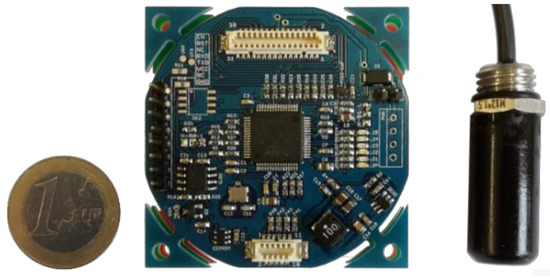
Figure 3.
AHOI acoustic underwater modem with an AS-1 hydrophone (and 1-euro coin).
Signal processing is realized in software on the microcontroller, which allows for a fast reconfiguration of frequency and coding setups. The AHOI modem uses a packet-based communication and each packet begins with a preamble and a start frame delimiter (SFD) to apply a per-packet synchronization. A packet consists of a header (containing 6 Byte of information plus an additional 1 Byte cyclic redundancy check (CRC) checksum) and payload (that uses an additional 2 Byte CRC checksum). In shallow-water scenarios, the acoustic wave is reflected at the surface and the bottom, and by several other objects, for example, quay walls and ships. The reflections lead to a multi-path propagation channel with frequency selectivity [45]. To counter time-dependent attenuation caused by multi-path propagation, each symbol is repeated three times. In addition, frequency hopping (FHSS) is applied using a hopping scheme, which is adapted to the symbol repetitions. The combination of repetitions and FHSS distributes the bits over a wider bandwidth and addresses frequency cancellations. Other configurations have been evaluated in References [7,46], where the proposed one has been proved to provide a good trade-off between data rate and communication reliability in various scenarios. All in all, the modem has 25 kHz bandwidth around a central frequency of 62.5 kHz. The default setup, in combination with an extended Hamming code, leads to a net data rate of 260 kbit/s. However, the actual firmware allows a net data rate up to 4.7 kbit/s using six bits per symbol (37.5 kHz bandwidth), 1.28 ms symbol duration, and without repetitions and Hamming coding. An extensive discussion about the different setups of the AHOI modem is provided in Reference [46].
3.1. AHOI Modem Performance in Very Shallow Water
A real-world evaluation was performed in a marina in southern Hamburg (cf. Figure 4). The marina is located in a branch of the river Elbe, where depth ranges from approximately 3.5 m to 7.5 m, depending on the tide. The experiments were performed on Nov. 11, 2018. It was a windless day and with small and infrequent waves. During the evaluation, the environmental data was recorded with a professional CTD-48 probe manufactured by Sea&Sun Technologies [47]. Water temperature was 9.9 °C and salinity was 0.68 ppt, resulting in a speed of sound of 1447.7 m/s.

Figure 4.
Nodes during the field test with five receivers ( to ) and a single transmitter ().
In total, six AHOI modems (used with the default configuration) were deployed on a jettie, one modem acted as sender and the other five as receivers. All hydrophones were submerged 1.5 m under the water surface and each modem was connected to a laptop to record the received packets. During the evaluation, packets with different payload lengths were transmitted. In each setup the transmitter sent 200 packets with randomly generated payload. After each transmission, the sender waited 150 ms in order to allow a channel cooldown phase between the transmissions. Table 1 contains the packet delivery ratio (PDR) of the five receivers for 4 Byte, 8 Byte, 16 Byte, and 32 Byte payloads.

Table 1.
Packet delivery ratio achieved during the real-world evaluation in a marina in Hamburg.
3.2. AHOI Modem’s Reaction to Shipping Noise
The typical range of applications of USNs includes marinas, ports and rivers with high shipping activity. Each ship or AUV produces acoustic noise caused by propellers, machineries and other effects [11]. For this reason, in order to provide a stable communication link in the port of Hamburg, the AHOI modem must be resilient against shipping noise. The acoustic noise emitted by vessels and ships have highest power spectral density (PSD) below 10 kHz, which is lower than the communication frequency range. In addition, the AHOI modem receiver involves a band-pass filter between 50 kHz and 75 kHz (cf. Section 3). However, a simulation was performed to prove the stability against shipping noise. The noise was generated offline with the help of the equations in Reference [11], and added to different recorded packets. The shipping noise was calculated for a 180 m long cargo vessel traveling at 15 knots, and for a Bluefin Robotics AUV. Simulated distances from the transmitter to the ship and the receiver were respectively , while the distances between AUV and receiver were . In both cases (ship and AUV noise), the noise sources were modeled as point sources. However, the ship noise was calculated for a 180 m long cargo vessel, which is larger than . In reality, the ship noise sources are distributed over the ship hull and the received signal level is lower. On the contrary, AUVs are smaller, and so are the distances : the case = 1 m simulates the case when the receiver is installed into the AUV itself.
The received signal strength was calculated with the spreading loss according to Reference [45], assuming a spherical spreading and free-field conditions. Based on that, all propagation paths besides the line-of-sight (LOS) were neglected and the relation between the attenuation and the distance d was approximated with . A single AHOI modem was used to receive the signal, which was generated with an arbitrary signal generator (TiePie Handyscope HS5, 200 kHz sampling). The signal generator simulated the received hydrophone voltage for different PSDs. During the simulations a constant receiving sensitivity of −208dB re 1V/μPa (cf. sensitivity of the Aquarian Audio AS-1 in Reference [44]) for frequencies up to 100 kHz was assumed. Figure 5 shows the PSDs of received packets and the perceived noise at the receiver side. At first, the packets were transmitted without additional noise. In the following simulations, different noise profiles were added to the packets. For each combination of noise level, noise source, and communication signal strength, 500 packets (with 32 Byte payload) were transmitted.
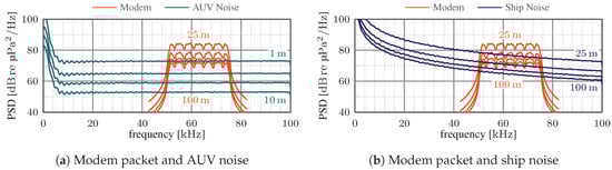
Figure 5.
Power spectral densities (PSDs) of the simulated modem signals and additional shipping noise. The PSDs correspond to received signals (packets or noise) with and distance to the transmitter or noise source.
The AUV noise affected the packet reception only in a single case, whereas in the other cases all transmitted packets were received. The combination and resulted in 99.8% received packets (only one packet was not received). Furthermore, Table 2 depicts the results of the shipping noise simulations. In most cases, also the shipping noise did not affect the PDR. However, the setup and resulted in a PDR of 36.2%.
Table 2.
Packet delivery ratio when simulating the presence of a 180 m cargo vessel (traveling at 15 knots) at different distances from the receiver (distance between transmitter and receiver , and between ship and receiver ).
Based on the simulations, the cargo ship noise starts to affect the packet reception only when the distance between the ship and the receiver is below or equal to 25 m, and the distance between the transmitter and the receiver is above 75 m.
3.3. Modem’s Reaction to Interference
In addition to the vessel noise discussed in Section 3.2, the signals generated by the other underwater modems in the network could also disturb the transmission. To evaluate the effect of packet interference and the resulting PDR, the hardware configuration described in Section 3.2 was used: in this case, a second recorded packet was added to the generator samples. All packets carried a 32 Byte payload and had a signal duration of 1.311 s, including the synchronization symbols.
The PDR has been measured by varying the interference power and overlap, and its performance mapped in the simulator. Specifically, the Signal to interference Ratio (SIR) component has been calculated by employing the mean power model, computed as
where is the power received by the signal carrying the data packet, the power of the interfering signal and the overlap of the two signals, calculated as the amount of time the two signals interfere divided by the total packet duration. The measurements have been interpolated by employing the Piecewise Cubic Hermite Interpolating Polynomial (PCHIP) with Matlab, obtaining the line depicted in Figure 6.
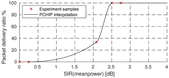
Figure 6.
Packet delivery ratio vs. Signal to Interference Ratio of the AHOI modem.
3.4. AHOI Performance Inclusion in the DESERT Underwater Network
In order to simulate the AHOI modem behavior, we developed a new physical layer module into the DESERT Underwater Network Simulator. The performance figures of the AHOI modem can be imported in this module in the form of lookup tables (LUTs). Specifically, the PDR versus distance presented in Table 1 has been mapped into a LUT to obtain the modem’s behavior in shallow water, in the absence of interference and shipping noise.
The PDR versus Signal to Vessel-Noise Ratio LUT obtained from Figure 5 and Table 2 has not been included in this work, as the effect of the vessel noise is negligible in the scenario of interest for this paper. Indeed, it is not likely that a cargo ship passes closer than 50 meters to a network deployment and the new version of the Bluefin Robotics AUV [11] has a propeller noise 15 dB lower then the model considered in Section 3.2.
The PDR versus Signal to Interference Ratio LUT (already presented in Figure 6), instead, has been included in the simulator, to obtain the penalty introduced by the interference. The resulting packet delivery ratio is approximated as
where is the packet delivery ratio obtained at a distance d, while is the packet delivery ratio obtained in ideal conditions with signal to interference ratio equals to SIR. A similar simulation approach was also used in Reference [14].
4. Protocols Description
This paper presents a hybrid multimodal network, composed by sensor nodes, an AUV and a sink node. The sensor nodes are equipped with the AHOI modem, while the sink uses the EvoLogics S2CM HS acoustic modem. The AUV collects the data from the sensors: it can behave as the sink itself, by resurfacing and transmitting the data to shore via radio link or convey the data to a sink deployed from a buoy or an Autonomous Surface Vehicle (ASV). In the former case, the AUV can be equipped only with the AHOI modem, while in the latter case it has to use an EvoLogics S2CM HS modem as well. In order to handle different modems the AUV requires a dedicated multimodal layer, that selects which modem to employ. This layer, called UW-MULTI-DESTINATION [48], is deployed between the routing layer and the MAC layer. For each incoming packet from the routing layer, UW-MULTI-DESTINATION first checks the packet’s next hop address and then chooses the right physical layer technology to use for the transmission. This selection is performed through a technology per node map, where the UW-MULTI-DESTINATION stores the list of physical layers available at each node. In our case this list is assumed to be known at network deployment, however, a periodic topology discovery mechanism [49] might be employed to update the list. In Section 7.1, a protocol stack that employs the UW-MULTI-DESTINATION layer will be evaluated via simulation.
UW-POLLING, the polling-based MAC protocol used in this USN, is presented in Section 4.1.
4.1. A Polling-Based Mac Protocol for Underwater Acoustic Networks
The MAC layer employed in the data-muling scenario is a polling-based MAC protocol. The general behavior of the protocols is described by the state machines depicted in Figure 7. In particular, most of the protocol logic is implemented in the AUV (Figure 7a), which collects the data from the sensor nodes and, optionally, forwards the data to a sink node. All the operations performed by the sensor nodes (Figure 7b) and the sink node (Figure 7c) are executed in reaction to the AUV indications.

Figure 7.
From left to right: state machine of the UW-POLLING protocol for an AUV (a), for a node (b) and for a sink (c), respectively.
The UW-POLLING protocol works in two phases: the discovery phase identifies how many surrounding sensor nodes have data packets to send and the polling phase collects the data from the nodes. In case a sink node is employed, in the polling phase the data is also forwarded to the sink. The discovery phase starts when the AUV sends a TRIGGER packet () in broadcast, revealing itself to all the surrounding nodes. Each node that correctly received the and has data to transmit replies with a PROBE packet () after a random backoff time. The AUV collects all the s and then starts the polling phase sending to one node at a time a POLL packet () and waiting for the data from the selected node. If the SINK receives a , it replies with a as well; afterwards, in the polling phase, the AUV will forward the data to the sink. A detailed description of the UW-POLLING protocol is reported in the rest of this section.
At the beginning of the discovery phase the AUV transmits the to all the surrounding nodes. The contains information that will be used by the nodes to send the . In particular, the minimum () and the maximum () backoff time to use for the transmission of the are inserted in the . This mechanism enables the AUV to possibly adapt the backoff time choice based on the network density.
The nodes that correctly received the and have data packets to send reply with the . Each node transmits the after a random backoff time uniformly chosen between and . In the , each node i inserts the number of data packets that is going to transmit () in the polling phase. This information is needed by the AUV to choose the order in which to poll the nodes. is bounded by a maximum value equal for each node of the network, in order to avoid that a node which holds many packets acquires the access to the channel for a long time, thereby preventing all the surrounding nodes from transmitting. If the sink received the , it takes part in the contention, transmitting a as well. The AUV waits for the reception of all the s until either a timeout expires or the maximum number of () is received.
Once the is transmitted, the node waits for the from the AUV. If the is not received before a timeout , the node considers a failure in the transmission of either the or the and waits for the reception of another . Similarly, the sink waits for for the reception of the first data packet from the AUV. If the data is not received within , the sink waits for the reception of another .
If the AUV does not receive s, the discovery phase starts again with the transmission of another . Instead, if at least one PROBE is received, the polling phase starts. Firstly, the AUV creates the POLL list, that is, the ordered list of the nodes to be polled. The UW-POLLING protocol sorts the nodes according to a proportional fair scheduling, trying to obtain fairness in the number of packets each node transmits to the AUV. In particular, for each node i, the AUV computes a weight , where is the number of data packets received by the AUV from node i so far [50]. Then the nodes are sorted according to this weight, in order to select first the nodes with the highest weight. If two or more nodes have the same weight, they are ordered depending on the time of arrival. If a from the sink is received, the sink is inserted in the list as well. The sink is inserted in the first position such that the sum of the packets that the AUV expects to receive from the previous nodes in the list and the number of data packets that are already in the AUV’s queue (), is greater than or equal to the maximum number of packets the AUV can transmit to the sink in each polling phase (). Thus, if m is the position in the POLL list, the sink is placed in position such that
If this condition is never reached, the sink is inserted at the end of the POLL list.
After the creation of the POLL list, the AUV starts to POLL all the nodes in the list. The AUV sends a to the first node in the list and waits for the reception of the data packets from the selected node. Once the AUV receives all the expected data packets from node i, it polls the next one in the list. If some packets are lost, the AUV waits until the timeout expires before going to the next node in the list. is automatically computed based on the number of data packets the AUV expects to receive from node i and the round-trip-time (RTT) between the AUV and the polled node, measured during the discovery phase.
In the the AUV inserts the expected amount of time it needs to poll all the nodes in the list. This value is used by all the nodes that received the POLL packet to refine the timeout . Similarly, the sink can use the value inserted in the POLL to adapt the timeout as well. When node i receives the intended for itself, it starts to transmit data packets to the AUV. After the transmission of the last packet, the node moves to the IDLE STATE waiting for the reception of another .
If the selected node in the list is the sink, the AUV starts to transmit up to data packets to the sink. Once the sink receives the first data packet, it refines the timeout to a value within which it expects to receive all the data packets from the AUV. The timeout is needed for the transmission of an acknowledgement (ACK) to the AUV. Indeed, if the last packet is lost, the sink needs to wait until expires before sending the ACK. Instead, if the last packet is correctly received the ACK is sent immediately after the reception of this packet. For this purpose, before sending the data, the AUV inserts in each packet a unique ID (UID) and the UID of the last packet it is going to transmit in that polling phase. The lost packets are sent again in the next polling phase, according to a Selective Repeat (SR) Automatic Repeat Request (ARQ) mechanism: after the data transmission, the sink sends to the AUV an ACK containing either the UIDs of the lost packets or the UID of the next expected packet, in case no packets are lost. The AUV waits for the reception of the ACK until seconds from the transmission of the last packet and, if the ACK is not received within this timeout, it considers the ACK lost and starts to POLL the next node in the list. Moreover, the sink employs a second mechanism for the packet acknowledgment. This second ACK is inserted in the and consists of a Go-Back-N (GBN) ARQ mechanism. Indeed, the transmitted by the sink contains the UID of the first lost packet in the previous polling phase. If no packets were lost, the UID of the next expected packet is inserted. The main purpose of the second ACK is to avoid the retransmission of the whole block of data packets in case the first ACK is lost.
When all the nodes in the POLL list are polled by the AUV, the polling phase ends and the discovery phase starts again.
4.1.1. Timeout Setting
As described in Section 4.1, the behavior of the UW-POLLING protocol depends on the timeout settings. In this section we describe more in detail how these timeouts are computed.
used by the AUV has to be properly set to a value such that all the s can reach the AUV before the timeout expires. In particular, the timeout has to be set to a value , where is the maximum RTT of a node in the network.
Another timeout employed in the protocol is . Each node updates its own timeout every time a is received. The value of is inserted in the and is computed each time a new is transmitted. The value of the timeout is computed as:
where is the number of remaining sensor nodes in the POLL list (the sink, if any, is not considered), is the time needed to transmit a DATA packet, is the RTT between node i and the AUV measured in the discovery phase and is a guard time, used to take into account the processing delay and errors in the RTT measurement. The last term of the equation takes into account the time the AUV should employ to transmit packets to the sink. The value of inserted in the is also used by the sink to update .
The timeout is also updated when the first data packet is received by the sink. The timeout is updated based on the number of data packets the sink is going to receive by the AUV. Since each data packet contains the UID of the last transmitted packet in that polling phase, the sink can easily compute the expected number of packets it will receive. The time needed to receive the data is and the timeout is set to:
Finally, is the timeout used by the AUV to stop waiting for the reception of the data packets from a polled node i and is computed as:
4.1.2. Choice of the Maximum Backoff Time
For each node density , defined as the number of nodes deployed in 1 km2, an optimal value for the maximum backoff time () that maximizes the throughput exists (see Section 5.2 and Section 6.2). If the AUV is not aware of the network node density, or if the density is not constant in all the network area, the AUV has to employ some algorithm to estimate the value of and, therefore, adapt the best maximum backoff time to use time by time. In this section, we present a reactive system based on the estimated number of neighbors . This estimate is performed by the AUV at the end of the discovery phase, by observing the number of probe packets received. Two separate cases are analyzed: the case where we assume full knowledge () information about the number of packets arrived at the physical layer and the realistic case (), where only the packets received by the MAC layer are considered.
- assumes full knowledge of the number of s that have been correctly received in the k-th discovery phase and the number of packets discarded () by the physical layer at any time during the simulation. While the former is a parameter well known by the MAC layer, the latter can rarely be determined with high accuracy by a real modem: for this reason the algorithm is used as an upper-bound benchmark. With , the estimated number of neighbors during the k-th discovery phase is calculated aswhere is the total number of lost packets at the beginning of the k-th discovery phase and the total number of lost packets at the end of the same discovery phase.
- assumes knowledge of and , that is, the number of probe packets that have been correctly received and discarded by the MAC layer in the k-th discovery phase, respectively. In this case, both parameters are known by the MAC layer of realistic modems, therefore we are not introducing any assumptions that may favor our solution (this is particularly true for both the AHOI and the EvoLogics modems, although the latter has to be employed with the extended notification activated). The estimated number of neighbors during the k-th discovery phase is calculated as
A packet is discarded by the MAC layer due to the failure of the CRC checksum, either because of low SNR, or because of interference. A packet is not received by the physical layer (and, consequently, not even passed to the MAC), instead, if its signal strength is below the sensitivity threshold of the transducer, due to a failure during the per-packet synchronization caused by a low SNR or interference, or if the packet reaches the destination when the physical layer is already receiving another packet. The last case is true only if the modem does not employ any interference cancellation mechanism [51] and preamble re-synchronization, as in the case of the AHOI modem. In order to perform a fair comparison, in this paper we assume that also the EvoLogics HS modem does not employ any interference cancellation system, as we do not have any information about it.
As presented in Equation (8), is calculated by accounting two times the number of packets discarded by the MAC layer: this is because during the discovery phase, where many nodes compete to access the channel, there is a high probability that if a packet is lost at the MAC layer this is due to the interference with another packet arrived after the beginning of the reception of . In this case, both and are discarded but only is detected. In the results we will analyze when this consideration is true and how it affects the system performance.
5. Protocol Evaluation in the Case of a High Speed Acoustic Modem
In this section, we evaluate the protocol in the case where both AUV and sensor nodes are equipped with EvoLogics S2CM HS acoustic modems. In this evaluation, the AUV acts as the sink itself. The performance of the protocol is evaluated by varying the node density , defined as the number of nodes deployed in 1 km2. The settings used for our simulations are presented in Section 5.1, while Section 5.2 reports the simulation results.
5.1. Simulation Scenarios and System Settings
The protocol stack implemented in the DESERT Underwater Network Simulator [16] for the sensor nodes and the AUV is depicted in Figure 8a,b, respectively. The physical layer employed in these simulations is the default physical layer of DESERT, which employs the propagation model presented in Reference [6]. In order to simulate the behavior of the EvoLogics S2CM HS modem [15], the center frequency has been set to 150 kHz, the bandwidth to 60 kHz, the transmission power to 156 dB re 1μ Pa@1m and the bitrate to 7 kbit/s. The payload packet length has been set to 125 Byte (plus additional 8 Byte needed for the headers of the protocol stack presented in Figure 8). With this configuration and, considering a shipping factor of 1, wind speed of 5 m/s and a geometrical spreading factor of 1.75, the maximum coverage range of the modem in our simulations is 490 m. This range is actually higher than the nominal range of this EvoLogics modem (that is 350 m in shallow water), because in this first simulation no multipath has been considered. A more realistic model has been considered in Section 7.
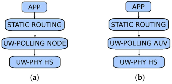
Figure 8.
Protocol stacks used by the sensor nodes (a) and the AUV (b), respectively, during the single mode scenario with the EvoLogics S2CM HS modem.
With this network configuration, two different scenarios are considered. In both scenarios, the AUV moves in a circular path of diameter D = 1000 m at a fixed speed of 2 m/s (the protocol reaction to the AUV speed has been already addressed in Reference [13]). In the first scenario, depicted in Figure 9a, the nodes are uniformly distributed in a 2D space according to a homogeneous Poisson point process (PPP) with density . In this case, the overall throughput of the network is analyzed by varying and , in order to find the value of that maximizes the throughput for each value of . These values are mapped in a LUT and used as an input for the simulations related to the second scenario (Figure 9b), where the nodes deployed along the AUV path have a variable density. In this case the value of ranges from 10 to 200 nodes/km2. Indeed, in the second scenario the behavior of the adaptive backoff algorithm is analyzed, comparing the two approaches (FC and RC) described in Section 4.1.2 with the fixed backoff case.
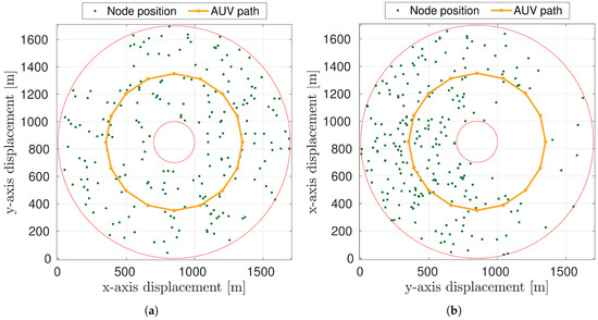
Figure 9.
Examples of scenarios with the high speed modem: node deployment with a fixed node density = 100 nodes/km2 (a) and node deployment with variable ranging from 10 to 200 nodes/km2 (b).
5.2. Results
In this section we report the results obtained with the high speed modem in the two scenarios described above. First of all, we analyzed the UW-POLLING protocol considering a fixed maximum backoff time and then we compared the different approaches employed to estimate the number of neighbors in the case of adaptive backoff time. All the results have been obtained averaging over 20 independent simulation runs.
In the first scenario with a fixed value of throughout a simulation run (Figure 9a), we analyzed how impacts the network performance. Figure 10a depicts the overall throughput of the network as a function of the maximum backoff time for different values of , from 5 to 250 nodes/km2. The throughput is computed as:
where is the overall number of packets received by the AUV during the simulation and is the duration of the simulation.
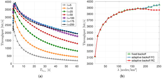
Figure 10.
Simulation results in the first scenario with high speed modem: overall throughput as a function of the maximum backoff time for different values of (a), throughput as a function of comparing adaptive backoff approaches and fixed backoff case (b).
With a value of 25 nodes/km2 the overall throughput decreases as the maximum backoff time increases. With these values of node density, the increase of the maximum backoff time leads to an increase of the time the AUV waits for the reception of the s, without significantly decreasing the collision probability and therefore without increasing the number of s correctly received. Conversely, for 25 nodes/km2 the overall throughput is a trade-off between the time the AUV waits for the reception of the and the number of s correctly received. With 25 nodes/km2, the maximum throughput value is equal to 3476 bit/s and is obtained with 0.5 s. With 50, 100, 175 nodes/km2 the maximum throughput (equal to 3673, 3826, 3876 bit/s, respectively) is reached with = 1 s. Considering a density 250 nodes/km2, the overall maximum throughput is equal to 3948 bit/s and is obtained with = 2 s. We want to highlight that the optimal maximum backoff time is always smaller than 2 s in this scenario, where the high speed modem is employed, because the propagation time plays an important role in avoiding collisions. Indeed, the time needed to transmit a is equal to 16 ms and in this amount of time acoustic waves cover a distance equal to 24 m, therefore 2 nodes whose distance from the receiver differs more than 24 m can transmit simultaneously without colliding at the receiver.
As a second step, we compared the maximum throughput obtained for each value of employing a fixed maximum backoff time with the throughput obtained choosing the maximum backoff time based on the estimate of the number of neighbors, considering the two approaches described in Section 4.1.2. As before, in this scenario we considered a network deployment with a fixed node density throughout each simulation run. The results are depicted in Figure 10b. The green line has been obtained taking the maximum value of the throughput for each from the previous results where a fixed was used. The blue line has been obtained considering the full knowledge (FC) approach in the estimate of the number of neighbors. This approach is used as a benchmark for the realistic case (RC) approach (red line), where only the packets discarded by the MAC layer are known. As we can observe, the results in the 3 cases are very similar with a node density 200 nodes/km2. With higher values of , the RC line starts to diverge from the other two cases. This is due to the error in the estimate of the number of neighbors in the realistic case. Indeed, in our algorithm we supposed that a packet is discarded at the MAC layer if a collision with another packet occurs. However, with such values of this assumption is no longer realistic, because there is a higher probability that a collision occurs between more than two packets.
As a last step, we analyzed the protocol in the second scenario (Figure 9b) where the value of changes in space. In this scenario we compared the throughput in 3 different cases: using a variable with the FC approach for the network density estimate, using a variable with the RC approach and using a constant value for the maximum backoff time lasting for the entire simulation run (AVG). In this last case, the value of is set as the optimal maximum backoff time for the average density of the network. The results, in terms of the overall throughput of the network, are depicted in Figure 11a. The difference between the full knowledge case (FC) and the AVG case in this scenario is only 10 bit/s. Indeed, the for the average case is equal to 1 s, that is a value suitable for the majority of the network densities analyzed in the previous scenario, that is, for all the between 45 and 175 nodes/km2. Figure 11b reports the optimal backoff time obtained via simulation as a function of the network density . This means that the adaptation of the maximum backoff time with the high speed modem is effective only with very low or very high network density. Moreover, as mentioned before, the RC approach is not able to properly estimate the number of nodes in a high density scenario, therefore, the results of the RC are closer to the AVG case rather than the to FC approach with the FC approach for the network density estimate, using a variable with the RC approach and using a constant value for the maximum backoff time lasting for the entire simulation run (AVG). In this last case, the value of is set as the optimal maximum backoff time for the average density of the network. The results, in terms of the overall throughput of the network, are depicted in Figure 11a. The difference between the full knowledge case (FC) and the AVG case in this scenario is only 10 bit/s. Indeed, the for the average case is equal to 1 s, that is a value suitable for the majority of the network densities analyzed in the previous scenario, that is, for all the between 45 and 175 nodes/km2. Figure 11b reports the optimal backoff time obtained via simulation as a function of the network density . This means that the adaptation of the maximum backoff time with the high speed modem is effective only with very low or very high network density. Moreover, as mentioned before, the RC approach is not able to properly estimate the number of nodes in a high density scenario, therefore, the results of the RC are closer to the AVG case rather than the to FC approach.
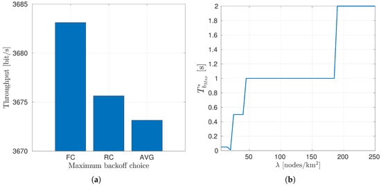
Figure 11.
Throughput in the variable density scenario with the adaptive backoff approaches (Full knowledge case and realistic case (FC and RC) and the fixed backoff case (AVG) (a). Optimal backoff time as a function of the network density obtained via simulation considering the first scenario with fixed node density (b).
6. Protocol Evaluation in the Case of a Low Rate Acoustic Modem
In this section, we evaluate the protocol in the case where both AUV and sensor nodes are equipped with AHOI acoustic modems. Similarly to Section 5.2, the AUV acts as the sink itself and the network performance is evaluated by varying the node density . The settings used for our simulations are presented in Section 6.1, while Section 6.2 reports the simulation results.
6.1. Simulation Scenarios and System Settings
The protocol stack implemented in the DESERT Underwater Network Simulator [16] for the sensor nodes and the AUV is depicted in Figure 12a,b, respectively. The physical layer employed in these simulations is the AHOI physical layer, described in Section 3. In this case, the central frequency has been set to 62.5 kHz, the bandwidth to 25 kHz, the transmission power to 156 dB re 1μPa@1m and the bitrate to 200 bit/s. The maximum coverage range of the AHOI modem is roughly 150 m. The payload packet length has been set to 24 Byte (plus additional 8 Byte needed for the headers of the protocol stack presented in Figure 12).
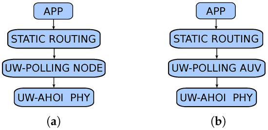
Figure 12.
Protocol stacks used by the sensor nodes (a) and the AUV (b), respectively, during the single mode scenario with the AHOI modem.
With this network configuration, two different scenarios are considered. In both scenarios, the AUV moves in a circular path of diameter D = 520 m at a fixed speed of 2 m/s (the protocol reaction to the AUV speed has been already addressed in Reference [14]). In the first scenario, depicted in Figure 13a, the nodes are uniformly distributed in a 2D space according to a homogeneous PPP, with a node density of nodes per square kilometer. Also in this case, the overall throughput of the network is analyzed by varying and , in order to find the value of that maximizes the throughput for each value of . These values are mapped in a LUT and used as an input for the simulations related to the second scenario (Figure 13b), where the number of nodes deployed along the AUV path has a variable density. In this case the value of ranges from 50 to 400 nodes/km2. Finally, in the second scenario the behavior of the adaptive backoff algorithm is analyzed comparing the FC and RC approaches (described in Section 4.1.2) with the fixed backoff case.
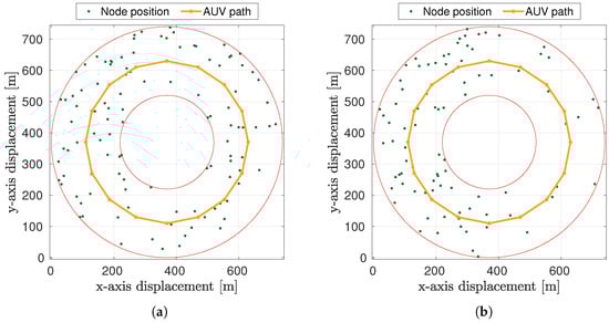
Figure 13.
Examples of the two scenarios considered in the low rate modem simulations: node deployment with a fixed node density = 300 nodes/km2 (a) and node deployment with variable ranging from 50 to 400 nodes/km2 (b).
6.2. Results
In this section, we present the performance of the UW-POLLING protocol in the first and second scenarios, when the low rate modem is employed. As for the high speed modem, we first analyzed the overall throughput of the network considering a fixed network density and a constant backoff time throughout a simulation run and then compared the different approaches to estimate the number of neighbors with both a fixed and a variable node density.
Figure 14a reports the overall throughput of the network as a function of the maximum backoff time for different values of . The throughput is computed as:
where is the overall number of packets received by the AUV during the simulation and is the duration of the simulation. In the low rate modem scenario the effectiveness of the maximum backoff time is more significant with respect to the high speed modem scenario. In this case the time needed to transmit a PROBE is equal to 0.56 s, that is bigger than the maximum propagation time experienced in this scenario (i.e., 0.1 s). This means that the distance between nodes is no longer sufficient to avoid collision unlike in the high speed scenario presented in Section 5. In this scenario, the maximum throughput is a trade-off between the number of PROBE packets correctly received and the time spent by the AUV waiting for the reception of the PROBE. With 25 the maximum throughput is obtained with 2 s. The optimal , that is, the maximum backoff time corresponding to the maximum throughput, increases as the network density increases.
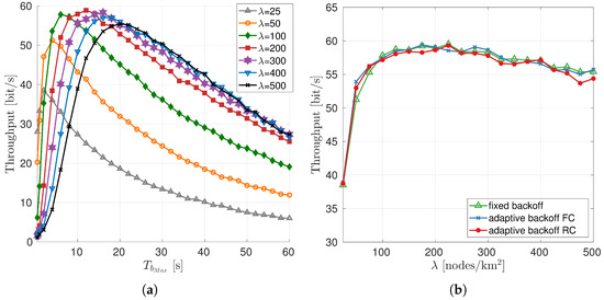
Figure 14.
Simulation results in the first scenario with low rate modem: overall throughput as a function of the maximum backoff time for different values of (a), throughput as a function of comparing adaptive backoff approaches and fixed backoff case (b).
In the scenario with fixed node density, we also compared the results obtained with the adaptive mechanisms for the choice of the maximum backoff time with the fixed . In the adaptive choice of the backoff we simulated both the FC approach, used as the upper-bound benchmark and the RC approach. Figure 14b depicts the results, in terms of throughput, in the three cases: fixed backoff (green line), FC approach (blue line) and RC approach (red line). The choice of the fixed maximum backoff has been obtained from the previous simulations with fixed density and fixed , selecting the maximum throughput for each . We can observe that the results in the three cases are almost equivalent for all values of . This means that the node estimate in the RC approach is accurate enough to not degrade significantly the performance with respect to the FC approach and with respect to the case where is known (fixed backoff case).
As a last step, we analyzed the protocol performance in the scenario with a variable node density (Figure 13b). Also in this scenario we compared the throughput in three different cases: using a variable with the FC approach for the network density estimate, using a variable with the RC approach and using a constant value for the maximum backoff time lasting for the entire simulation run (AVG). In the AVG case, the value of is set as the optimal maximum backoff time for the average node density of the network. The results, in terms of the overall throughput of the network, are depicted in Figure 15. In this scenario, where the low rate modem is employed, the throughput of the RC approach is very close to the benchmark obtained with the FC approach. Moreover, the improvement in the adaptive backoff case with respect to the AVG case is about 8%
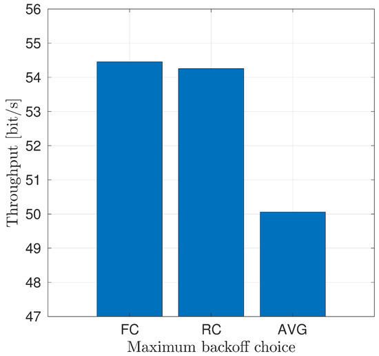
Figure 15.
Throughput in the variable density scenario with the adaptive backoff approaches (FC and RC) and the fixed backoff case (AVG).
7. Protocol Evaluation in a Multimodal Scenario
In this section we analyze the UW-POLLING protocols in the scenario of the port of Hamburg. Differently from the previous scenarios, in this deployment we considered a multimodal setting where both the AHOI modem and the EvoLogics S2CM HS modems are employed. Moreover, we considered a sink node placed in a fixed position and different from the AUV. The scenario and the setting employed in these simulations are presented in Section 7.1. Section 7.2 reports the results.
7.1. Simulation Scenarios and System Settings
In this scenario we considered a multimodal network where both the AHOI and EvoLogics modems are employed. Figure 16 reports the protocol stack for all the nodes in the network. In particular, sensor nodes are equipped with the AHOI modem (Figure 16a), the sink node is equipped with the high speed modem (Figure 16c) and the AUV is equipped with both modems (Figure 16b). The AUV protocol stack includes the UW-MULTI-DESTINATION layer (described in Section 4) for selecting which modem to employ at each packet transmission. Specifically, in the AUV the AHOI modem is used to collect the data from the sensor nodes deployed along the AUV path and the Evologics HS modem to forward the data to the sink, if in range. The AHOI modem has been simulated as described in Section 3, while for the EvoLogics HS modem, the acoustic propagation has been simulated with the Bellhop ray tracer, importing the Hamburg port bathymetry (Figure 17b) in the WOSS Framework [52]. Two instances of the UW-POLLING protocol have been used in the AUV protocol stack: one related to the AHOI modem and the other to the high speed modem.
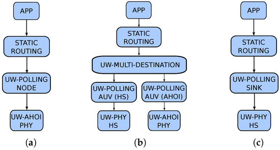
Figure 16.
Protocol stack used by the sensor nodes (a), the AUV (b) and the sink (c), during the complete multimodal scenario, where the AUV delivers the collected data to the sink.
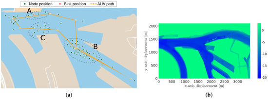
Figure 17.
Node deployment along the Elbe river in the port of Hamburg (a). Three clusters of nodes are identified with the letters A, B and C. (b) represents the port of Hamburg bathymetry related to the zone depicted in (a).
In this scenario, we deployed the nodes as in Figure 17a and we let the AUV move at 2 m/s, performing 10 laps of the orange path. We considered 63 sensor nodes deployed in an area of 0.6 km2 (average node density 105 nodes/km2), creating high density areas interspersed with low density areas. The sink (red node) is placed in a fixed position.
The UW-POLLING protocol related to the AHOI modem has been analyzed both with the adaptive backoff mechanisms (FC and RC) and in the fixed backoff case. In the fixed backoff case we use as the optimal value for the average node density obtained with simulations in the scenario described in Section 6.1. The optimal value with 105 nodes/km2 is equal to 6 s. The instance of UW-POLLING related to the EvoLogics modem has been analyzed considering only a fixed 20 s and with 1.
7.2. Results
In this section we present the results obtained in the scenario of the port of Hamburg described above.
Figure 18 reports the overall throughput of the network as a function of the overall offered traffic of the network G. The throughput is computed as:
where is the overall number of packets received by the SINK during the simulation and is the duration of the simulation. We assessed the performance of UW-POLLING considering the adaptive backoff mechanisms (FC and RC) and the fixed backoff case. In the adaptive backoff cases, the FC approach and the RC approach, used for the neighbors estimate, are almost equivalent. As mentioned in Section 6.2, with the AHOI modem the neighbors estimate performed with the RC approach is accurate enough to not degrade the performance in terms of throughput. The throughput increases as the offered traffic increases up to 300 bit/s. Considering 300 bit/s, the overall throughput of the network remains almost constant at 40 bit/s. For low values of G the difference between offered traffic and throughput is mainly due to packet losses due to bad channel conditions. Increasing G, the maximum achievable throughput is also limited by the bitrate of the modem and the presence of the discovery phase: for this reason, some of the nodes are not able to transmit all the generated packets to the AUV. In particular, in the area with high density nodes, such as cluster B, most of the packets remain in the node queues. In the low density areas this fact is less marked but still present. Thanks to multimodality, the transmission of the packets from the AUV to the sink is no longer a bottleneck, unlike what happened in Reference [14] where only the AHOI modem was employed. Moreover, also the fairness of the nodes is enhanced with respect to the results in Reference [13]. In that paper, nodes close to the sink were not able to transmit their data packets, because in their proximity the AUV was busy forwarding the data to the sink. With a multimodal approach, instead, we are able to both collect the data from sensor nodes and forward packets to the sink at the same time. In the fixed backoff case, the behavior is the same as for the adaptive mechanisms but the throughput is much lower than in the former cases: in particular, using an adaptive mechanism we can improve the performance up to 9%.
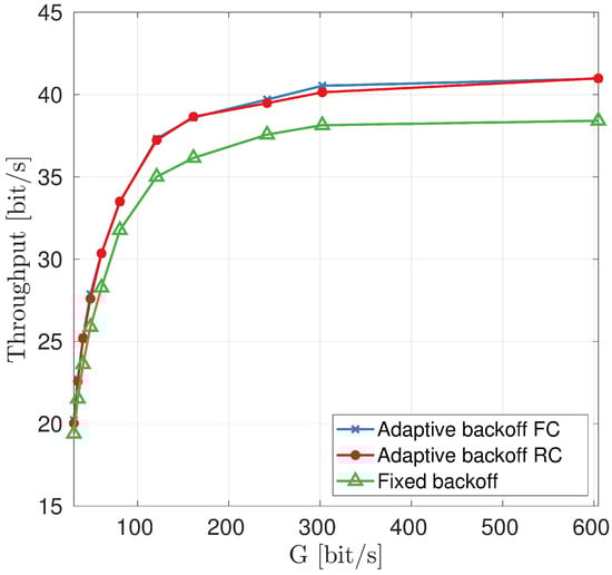
Figure 18.
Overall throughput in the port of Hamburg scenario as a function of the offered traffic.
Figure 19 reports Jain’s Fairness Indexes (JFIs) [53] as a function of the offered traffic, computed for both the overall network and the clusters of nodes depicted in Figure 17a. Jain’s Fairness index is computed as
where is the number of nodes in the network (or in the considered cluster) and is the number of DATA packets received by the AUV from node i. Figure 19a reports JFI for the whole network for both the adaptive backoff cases and the fixed backoff mechanism. In the adaptive cases JFI is slightly higher than in the fixed case, however in all cases, as the offered traffic increases JFI decreases, down to 0.6. Since the node density is not constant in space, we have to highlight that JFI of the whole network cannot be close to 1, especially for the largest values of offered traffic. Indeed the number of packets transmitted by a node in a high density area is smaller than the packets transmitted by a node in a low density area. For this reason we computed JFI separately for nodes in each of the clusters presented in Figure 17a. Figure 19b depicts JFI for the nodes in cluster A. Cluster A is representative of a low density scenario and JFI is close to 1 for both the adaptive backoff mechanisms and the fixed backoff case. Cluster B is a high density area and JFI in this area is depicted in Figure 19d. In this area JFI with both the FC and RC approaches is equal to 0.85 for 100 bit/s. As G decreases, JFI further increases up to 1. Therefore, also in high density scenarios we are able to obtain a good level of fairness. In the fixed backoff case, with 100 bit/s JFI decreases down to 0.75. The difference between the adaptive cases and the fixed backoff case is because the used in the fixed case is not suitable for this area. Indeed, the node density in this area is about 235 nodes/km2 and the maximum backoff time is too small, causing a higher collision probability for the s and therefore giving less chance to the nodes to transmit their packets. Finally, Figure 19d reports JFI computed for the nodes in cluster C. In this case JFI is similar for all the three assessed cases. JFI decreases for G smaller than 150 bit/s and then remains constant to 0.86 for bigger values of the offered traffic.
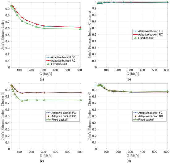
Figure 19.
Jain’s Fairness Index for the whole network (a), cluster A (b), cluster B (c) and cluster C (d).
8. Conclusions
In this paper, we presented the performance evaluation of the UW-POLLING protocol in a high density acoustic network. We assessed the protocol in a data-muling scenario where an AUV collects the data from sensor nodes and forwards the data to the shore, either resurfacing and transmitting the data itself, or forwarding the data via acoustics to a sink node directly connected to the shore with a radio link. We analyzed how the protocol performance is impacted by the choice of the maximum backoff time and how an adaptive strategy can be effective when the node density is either unknown, or not constant across the network area.
First of all, we analyzed the performance in a scenario with a uniformly distributed node deployment considering the nodes equipped with the EvoLogics S2C HS acoustic modem. We found, via simulation, the optimal backoff values for different fixed node densities. With the high rate modem, the backoff time does not have a big impact on the network performance: 2 s is a value that basically maximizes the throughput for all the analyzed node densities. Moreover, we compared the fixed backoff strategy with two adaptive approaches based on the estimate of the number of neighbors: the full knowledge case (FC), used as a benchmark and the realistic case (RC). We found that with node densities ≤ 200 nodes/km2 the performance in the three cases (fixed backoff, FC and RC) is equivalent.
Since commercial off-the shelf modems are too expensive for an actual dense node deployment in a civilian scenario, we also evaluated the UW-POLLING protocol performance with the low-cost, low-rate and vessel-noise resistant AHOI modem, developed by the Technical University of Hamburg. Also in this case, we identified the optimal maximum backoff time in a scenario with uniformly distributed nodes, considering different node densities. Differently from the high rate modem, in this scenario the maximum backoff time plays an important role in avoiding the collisions of PROBE packets and, therefore, in increasing the overall throughput of the network. Also in this case we compared the fixed backoff case with the adaptive cases. We considered the three different approaches (fixed backoff, FC and RC) in a scenario with both fixed and variable node density. In the variable density case, with the adaptive mechanisms we obtained an improvement in the overall throughput of about 8% compared to the fixed backoff case.
Lastly, we evaluate the protocol performance in the scenario of the port of Hamburg. In this scenario, a multimodal solution was employed to collect data from sensor nodes and forward it to the sink. To better simulate the channel conditions for the high speed modem, we employed the WOSS framework using the Bellhop ray tracer and the bathymetry of the port of Hamburg. We analyzed the overall throughput of the network and the fairness for the sensor nodes as a function of the offered traffic. In particular, we observed the fairness for three clusters of nodes, each one with a different node density. Our results showed that an adaptive backoff mechanism not only increases the overall throughput of the network but also allows to achieve a better level of fairness in the areas with a high node density than in the fixed backoff case.
In this paper we proved via field measurements-based simulations that the AHOI modem can be used to retrieve data from a dense underwater sensor network deployment. This modem is very low cost but still requires the use of an off-the shelf transducer, whose price is twice the cost of the modem itself. In our ongoing works, we will study how to cut the transducer cost, building a transducer in-house, which we hope will result in a 50% reduction of the overall cost of a real deployment. In addition, for future works, real field-experiments in the Elbe river will be performed to verify the effectiveness of the proposed solution to retrieve data from submerged sensors.
Author Contributions
Conceptualization, F.C. and A.S.; methodology, A.S., F.C. and F.S.; data curation, A.S. and F.S.; investigation, A.S. and F.S.; formal analysis, A.S. and F.C.; software, A.S.; validation, F.C.; writing—original draft preparation, F.C. and A.S.; supervision, B.-C.R. and M.Z.; resources, F.S., B.-C.R. and M.Z.; visualization, A.S., F.C. and F.S.; project administration, F.C., B.-C.R. and M.Z.; funding acquisition, F.C., B.-C.R. and M.Z.
Funding
This research was funded in part by the Italian Ministry of Education, University and Research (MIUR), the German Federal Ministry for Economic Affairs and Energy (BMWi, FKZ 03SX463C), and ERA-NET Cofound MarTERA (contract 728053).
Acknowledgments
The authors would like to thank the Hamburg Port Authority (HPA) that provided the bathymetry and the sound speed profile data used in the simulations of this paper, and Federico Favaro and Federico Guerra who reviewed our code and maintain the DESERT Underwater and the WOSS simulation frameworks.
Conflicts of Interest
The authors declare no conflict of interest.
Abbreviations
The following abbreviations are used in this manuscript:
| TRIGGER packet, sent by the AUV to the nodes | |
| PROBE packet, sent by the nodes to the AUV | |
| POLL packet, sent by the AUV to the nodes | |
| Minimum backoff time a node waits before transmitting a | |
| Maximum backoff time a node waits before transmitting a | |
| Number of data packets node i is going to transmit | |
| Maximum number of packets a node can transmit in a polling phase | |
| Maximum number of PrP AUV can receive in a discovery phase | |
| Total number of packets received by AUV from node i | |
| Maximum number of packets AUV can transmit to sink in a polling phase | |
| Node density, that is, the average number of nodes deployed in 1 km2 |
References
- Heidemann, J.; Stojanovic, M.; Zorzi, M. Underwater sensor networks: Applications, advances and challenges. Philos. Trans. R. Soc. A 2012, 370, 158–175. [Google Scholar] [CrossRef] [PubMed]
- Folaga Data Sheet. Available online: https://www.graaltech.com/folaga-features (accessed on 30 November 2019).
- Campagnaro, F.; Francescon, R.; Casari, P.; Diamant, R.; Zorzi, M. Multimodal Underwater Networks: Recent Advances and a Look Ahead. In Proceedings of the International Conference on Underwater Networks & Systems (WUWNET’17), Halifax, NS, Canada, 6–8 November 2017. [Google Scholar]
- Signori, A.; Campagnaro, F.; Zorzi, M. Modeling the Performance of Optical Modems in the DESERT Underwater Network Simulator. In Proceedings of the Fourth Underwater Communications and Networking Conference (UComms), Lerici, Italy, 28–30 August 2018. [Google Scholar]
- Chitre, M.; Shahabudeen, S.; Stojanovic, M. Underwater Acoustic Communications and Networking: Recent Advances and Future Challenges. Mar. Tech. Soc. J. 2008, 42, 103–116. [Google Scholar] [CrossRef]
- Stojanovic, M. On the Relationship Between Capacity and Distance in an Underwater Acoustic Communication Channel. SIGMOBILE Mob. Comput. Commun. Rev. 2007, 11, 34–43. [Google Scholar] [CrossRef]
- Renner, C.; Golkowski, A.J. Acoustic Modem for Micro AUVs: Design and Practical Evaluation. In Proceedings of the 11th ACM International Conference on Underwater Networks & Systems, Shanghai, China, 24–26 October 2016. [Google Scholar]
- Develogic Subsea Systems. Available online: http://www.develogic.de/ (accessed on 30 November 2019).
- S2CR 18/34 Acoustic Modem. Available online: http://www.evologics.de/en/products/acoustics/s2cr_18_34.html/ (accessed on 30 November 2019).
- Teledyne-Benthos Acoustic Modems. Available online: https://teledynebenthos.com/product_dashboard/acoustic_modems (accessed on 30 November 2019).
- Coccolo, E.; Campagnaro, F.; Signori, A.; Favaro, F.; Zorzi, M. Implementation of AUV and Ship Noise for Link Quality Evaluation in the DESERT Underwater Framework. In Proceedings of the Thirteenth ACM International Conference on Underwater Networks & Systems, Shenzhen, China, 3–5 December 2018. [Google Scholar]
- Akyildiz, I.F.; Pompili, D.; Melodia, T. Underwater Acoustic Sensor Networks: Research Challenges. Ad Hoc Netw. 2005, 3, 257–279. [Google Scholar] [CrossRef]
- Signori, A.; Campagnaro, F.; Zordan, D.; Favaro, F.; Zorzi, M. Underwater Acoustic Sensors Data Collection in the Robotic Vessels as-a-Service Project. In Proceedings of the MTS/IEEE OCEANS, Marseille, France, 17–20 June 2019. [Google Scholar]
- Campagnaro, F.; Steinmetz, F.; Signori, A.; Zordan, D.; Renner, B.C.; Zorzi, M. Data Collection in Shallow Fresh Water Scenarios with Low-Cost Underwater Acoustic Modems. In Proceedings of the International Conference and Exhibition on Underwater Acoustics, UACE2019, Crete, Greece, 30 June–5 July 2019. [Google Scholar]
- EvoLogics S2C M HS Modem. Available online: http://www.evologics.de/en/products/acoustics/s2cm_hs.html (accessed on 30 November 2019).
- Campagnaro, F.; Francescon, R.; Guerra, F.; Favaro, F.; Casari, P.; Diamant, R.; Zorzi, M. The DESERT Underwater Framework v2: Improved Capabilities and Extension Tools. In Proceedings of the Third Underwater Communications and Networking Conference (UComms), Lerici, Italy, 30 August–1 September 2016. [Google Scholar]
- Diamant, R.; Casari, P.; Campagnaro, F.; Zorzi, M. Leveraging the Near–Far Effect for Improved Spatial-Reuse Scheduling in Underwater Acoustic Networks. IEEE Trans. Wirel. Commun. 2017, 16, 1480–1493. [Google Scholar] [CrossRef]
- Campagnaro, F.; Guerra, F.; Diamant, R.; Casari, P.; Zorzi, M. Implementation of a Multi-Modal Acoustic-Optic Underwater Network Protocol Stack. In Proceedings of the OCEANS, Shanghai, China, 10–13 April 2016. [Google Scholar]
- Favaro, F.; Casari, P.; Guerra, F.; Zorzi, M. Data Upload from a Static Underwater Network to an AUV: Polling or Random Access? In Proceedings of the OCEANS, Yeosu, Korea, 21–24 May 2012. [Google Scholar]
- Peleato, B.; Stojanovic, M. Distance aware collision avoidance protocol for ad hoc underwater acoustic sensor networks. IEEE Commun. Lett. 2007, 11, 1025–1027. [Google Scholar] [CrossRef]
- Liu, W.; Weaver, J.; Weaver, L.; Whelan, T.; Bagrodia, R.; Forero, P.A.; Chavez, J. APOLL: Adaptive Polling for Reconfigurable Underwater Data Collection Systems. In Proceedings of the MTS/IEEE Kobe Techno-Oceans (OTO), Kobe, Japan, 28–31 May 2018. [Google Scholar]
- Nam, H. Data-Gathering Protocol-Based AUV Path-Planning for Long-Duration Cooperation in Underwater Acoustic Sensor Networks. IEEE Sens. J. 2018, 18, 8902–8912. [Google Scholar] [CrossRef]
- Pescosolido, L.; Petrioli, C.; Picari, L. A multi-band Noise-aware MAC protocol for underwater acoustic sensor networks. In Proceedings of the IEEE 9th International Conference on Wireless and Mobile Computing, Networking and Communications (WiMob), Lyon, France, 7–9 October 2013. [Google Scholar]
- Campagnaro, F.; Favaro, F.; Guerra, F.; Calzado, V.S.; Zorzi, M.; Casari, P. Simulation of Multimodal Optical and Acoustic Communications in Underwater Networks. In Proceedings of the OCEANS, Genova, Italy, 18–21 May 2015. [Google Scholar]
- Han, S.; Noh, Y.; Liang, R.; Chen, R.; Cheng, Y.J.; Gerla, M. Evaluation of underwater optical-acoustic hybrid network. IEEE China Commun. 2014, 11, 1518–1547. [Google Scholar]
- Basagni, S.; Blöni, L.; Gjanci, P.; Petrioli, C.; Phillips, C.A.; Turgut, D. Maximizing the value of sensed information in underwater wireless sensor networks via an autonomous underwater vehicle. In Proceedings of the IEEE INFOCOM 2014—IEEE Conference on Computer Communications, Toronto, ON, Canada, 27 April–2 May 2014. [Google Scholar]
- Gjanci, P.; Petrioli, C.; Basagni, S.; Phillips, C.A.; Boloni, L.; Turgut, D. Path Finding for Maximum Value of Information in Multi-Modal Underwater Wireless Sensor Networks. IEEE Trans. Mob. Comput. 2017, 17, 404–418. [Google Scholar] [CrossRef]
- Kaushal, H.; Kaddoum, G. Underwater Optical Wireless Communication. IEEE Access 2016, 4, 1518–1547. [Google Scholar] [CrossRef]
- Anguita, D.; Brizzolara, D.; Parodi, G.; Hu, Q. Optical wireless underwater communication for AUV: Preliminary simulation and experimental results. In Proceedings of the IEEE/OES Oceans, Santander, Spain, 6–9 June 2011. [Google Scholar]
- Subnero. Available online: https://subnero.com/ (accessed on 30 November 2019).
- MATS 3G Multi-Modulation Acoustic Telemetry System. Available online: http://www.sercel.com/products/Pages/mats3g.aspx (accessed on 30 November 2019).
- LinkQuest Underwater Acoustic Modems. Available online: http://www.link-quest.com/html/models1.htm (accessed on 30 November 2019).
- Beaujean, P.P.; Spruance, J.; Carlson, E.A.; Kriel, D. HERMES—A high-speed acoustic modem for real-time transmission of uncompressed image and status transmission in port environment and very shallow water. In Proceedings of the MTS/IEEE OCEANS, Quebec City, QC, Canada, 15–18 September 2008. [Google Scholar]
- Pelekanakis, C.; Stojanovic, M.; Freitag, L. High rate acoustic link for underwater video transmission. In Proceedings of the Oceans 2003. Celebrating the Past... Teaming Toward the Future (IEEE Cat. No.03CH37492), San Diego, CA, USA, 22–26 September 2003. [Google Scholar]
- Demirors, E.; Shankar, B.G.; Santagati, G.E.; Melodia, T. SEANet: A Software-Defined Acoustic Networking Framework for Reconfigurable Underwater Networking. In Proceedings of the 10th International Conference on Underwater Networks & Systems, ACM WUWNet, Arlington, VA, USA, 22–24 October 2015. [Google Scholar]
- Shimura, T.; Kida, Y.; Deguchi, M. High-rate acoustic communication at the data rate of 69 kbps over the range of 3600 m developed for vertical uplink communication. In Proceedings of the MTS/IEEE OCEANS, Marseille, France, 17–20 June 2019. [Google Scholar]
- Underwater Wireless Acoustic Video Communications Channel. Available online: http://www.baltrobotics.com/index.php/products-services-mnu/item/269-underwater-wireless-acoustic-video-communications-channel (accessed on 30 November 2019).
- Sherlock, B.; Neasham, J.A.; Tsimenidis, C.C. Implementation of a spread-spectrum acoustic modem on an android mobile device. In Proceedings of the MTS/IEEE OCEANS, Aberdeen, UK, 19–22 June 2017. [Google Scholar]
- Low Cost Underwater Acoustic Modem for Makers of Underwater Things and OEMs! Available online: https://dspcommgen2.com/news-flash-low-cost-acoustic-modems-and-transducers-available-for-sale-now/ (accessed on 30 November 2019).
- Cario, G.; Casavola, A.; Lupia, M.; Rosace, C. SeaModem: A Low-Cost Underwater Acoustic Modem for Shallow Water Communication. In Proceedings of the OCEANS, Genova, Italy, 18–21 May 2015. [Google Scholar]
- Sanchez, A.; Blanc, S.; Yuste, P.; Perles, A.; Serrano, J.J. An Ultra-Low Power and Flexible Acoustic Modem Design to Develop Energy-Efficient Underwater Sensor Networks. Sensors 2012, 12, 6837–6856. [Google Scholar] [CrossRef] [PubMed]
- Morozs, N.; Mitchell, P.D.; Zakharov, Y.; Mourya, R.; Petillot, Y.R.; Gibney, T.; Dragone, M.; Sherlock, B.; Neasham, J.A.; Tsimenidis, C.C.; et al. Robust TDA-MAC for practical underwater sensor network deployment: Lessons from USMART sea trials. In Proceedings of the Thirteenth ACM International Conference on Underwater Networks & Systems, ACM WUWNet, Shenzhen, China, 3–5 December 2018. [Google Scholar]
- Benson, B.; Li, Y.; Faunce, B.; Domond, K.; Kimball, D.; Schurgers, C.; Kastner, R. Design of a Low-Cost Underwater Acoustic Modem. IEEE Embed. Syst. Lett. 2010, 2, 58–61. [Google Scholar] [CrossRef]
- Aquarian Audio & Scientific. AS-1 Hydrophone. Available online: http://www.aquarianaudio.com/as-1-hydrophone.html (accessed on 30 November 2019).
- Stojanovic, M.; Preisig, J. Underwater acoustic communication channels: Propagation models and statistical characterization. IEEE Commun. Mag. 2009, 47, 84–89. [Google Scholar] [CrossRef]
- Steinmetz, F.; Renner, C. Resilience against Shipping Noise and Interference in Low-Power Acoustic Underwater Communication. In Proceedings of the MTS/IEEE OCEANS, Seattle, WA, USA, October 2019; Available online: http://www.bcrenner.de/publications/2019_OCEANS_ModemNoise.pdf (accessed on 30 November 2019).
- Sea & Sun Technology GmbH. Available online: https://www.sea-sun-tech.com/product/multiparameter-probe-ctd-48/ (accessed on 30 November 2019).
- Rizzo, W.; Signori, A.; Campagnaro, F.; Zorzi, M. AUVs Telemetry Range Extension through a Multimodal Underwater Acoustic Network. In Proceedings of the IEEE/MTS OCEANS, Charleston, SC, USA, 22–25 October 2018. [Google Scholar]
- Diamant, R.; Francescon, R.; Zorzi, M. Topology-Efficient Discovery: A Topology Discovery Algorithm for Underwater Acoustic Networks. IEEE J. Ocean. Eng. 2018, 43, 1200–1214. [Google Scholar] [CrossRef]
- Miao, G.; Zander, J.; Sung, K.W.; Slimane, S.B. Fundamentals of Mobile Data Networks; Cambridge University Press: Cambridge, UK, 2016. [Google Scholar]
- Diamant, R. Robust Interference Cancellation of Chirp and CW Signals for Underwater Acoustics Applications. IEEE Access 2018, 6, 4405–4415. [Google Scholar] [CrossRef]
- The World Ocean Simulation System—WOSS. Available online: http://telecom.dei.unipd.it/ns/woss/ (accessed on 30 November 2019).
- Le Boudec, J.-Y. Performance Evaluation of Computer and Communication Systems; Epfl Press: Boca Raton, FL, USA, 2011. [Google Scholar]
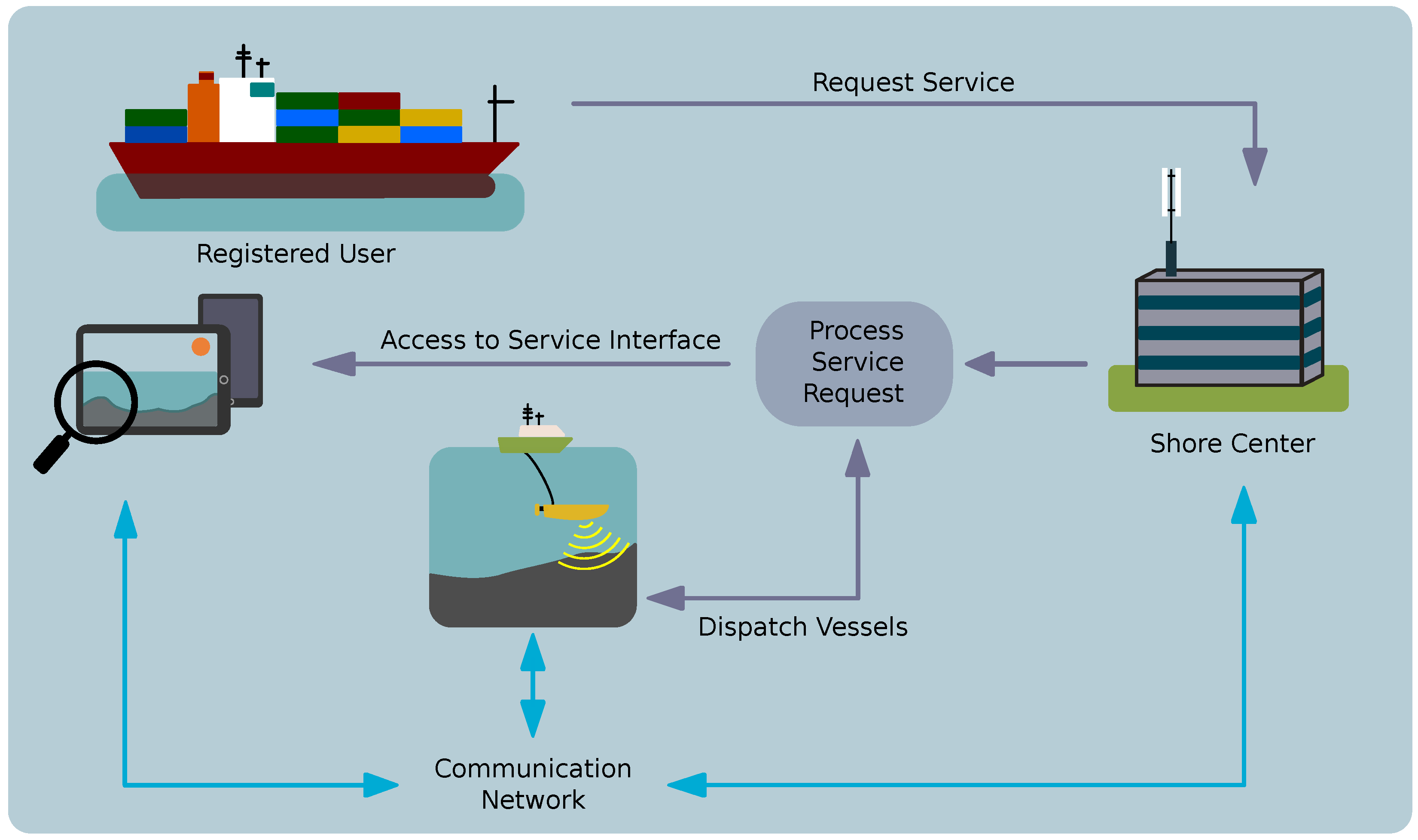


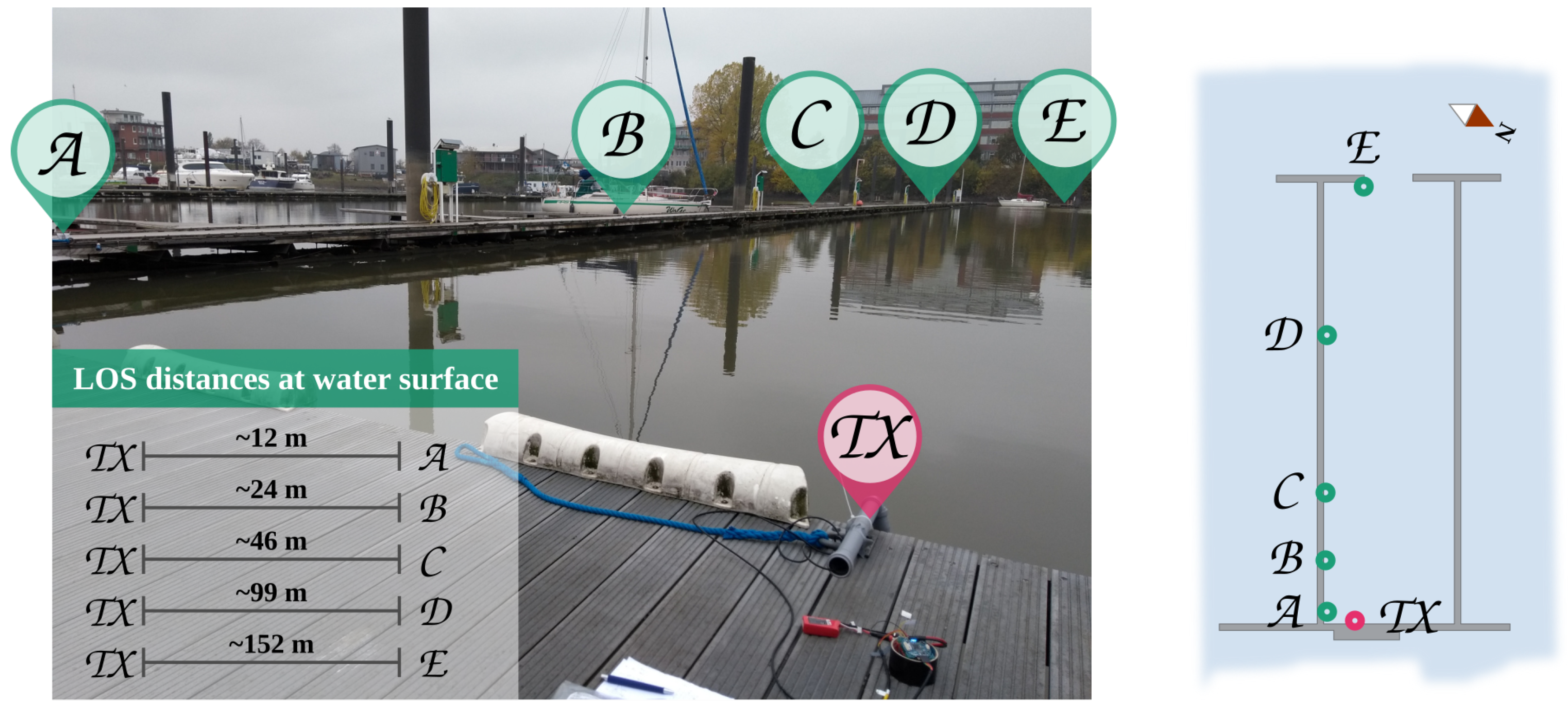
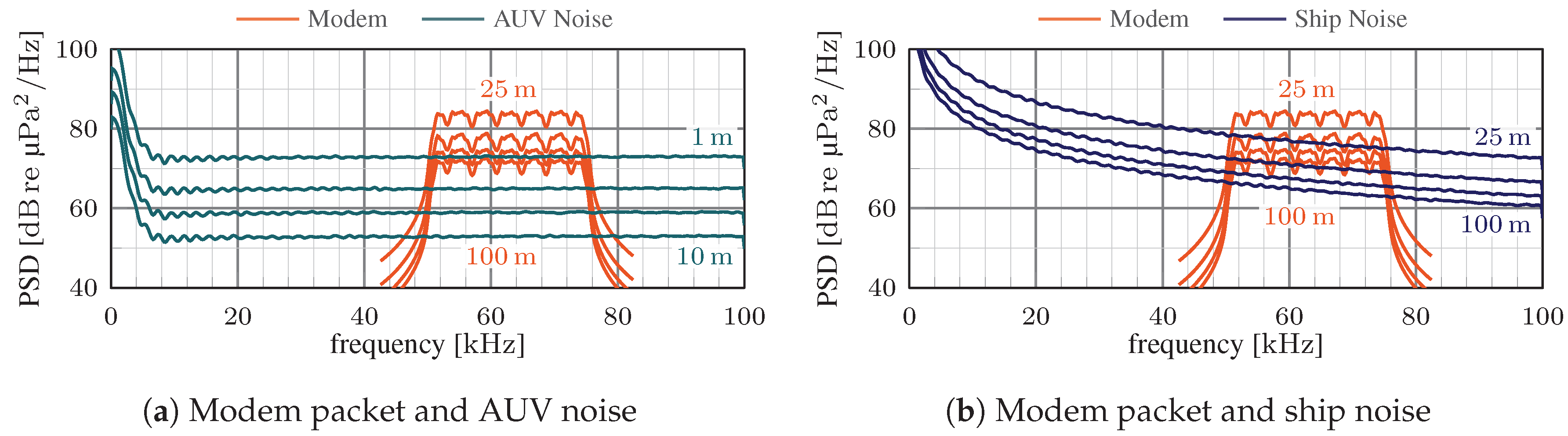
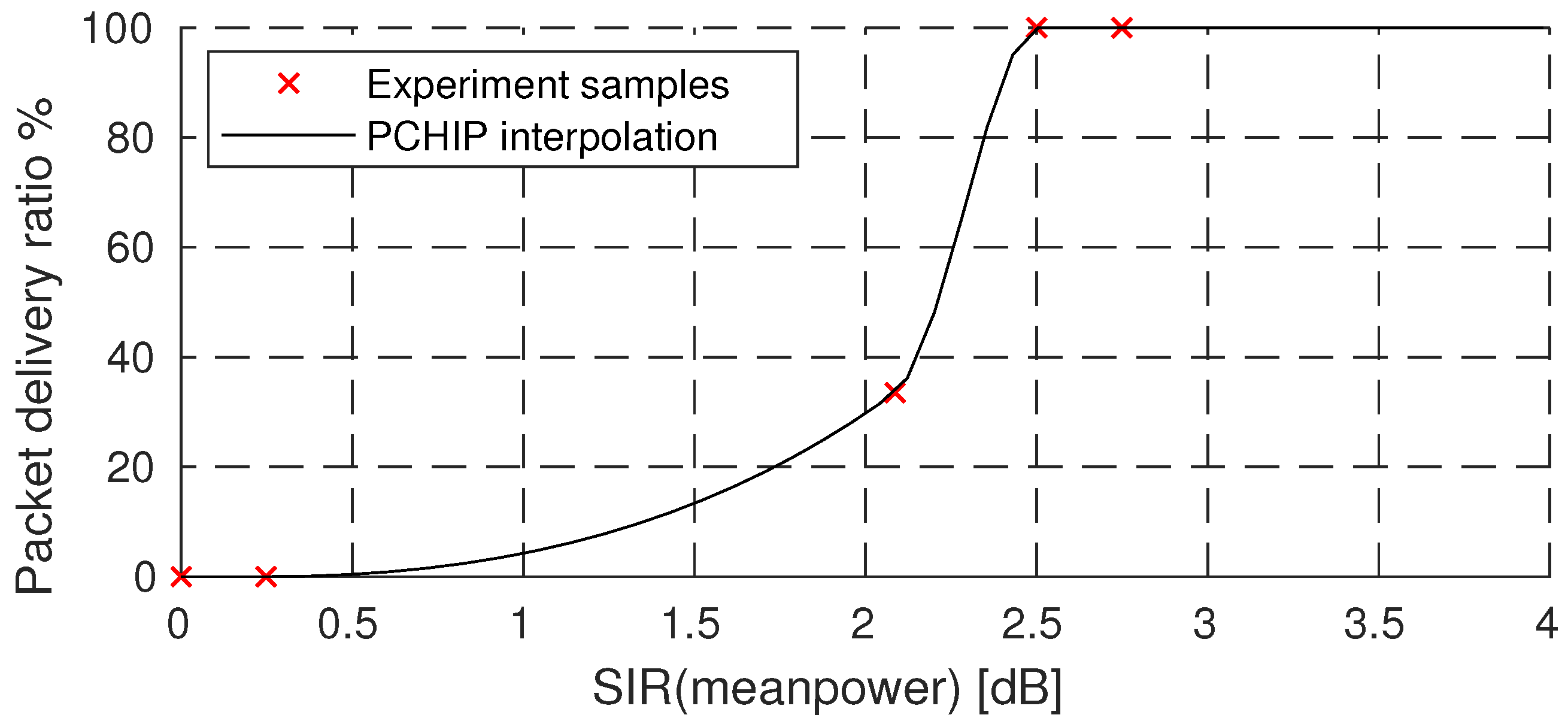
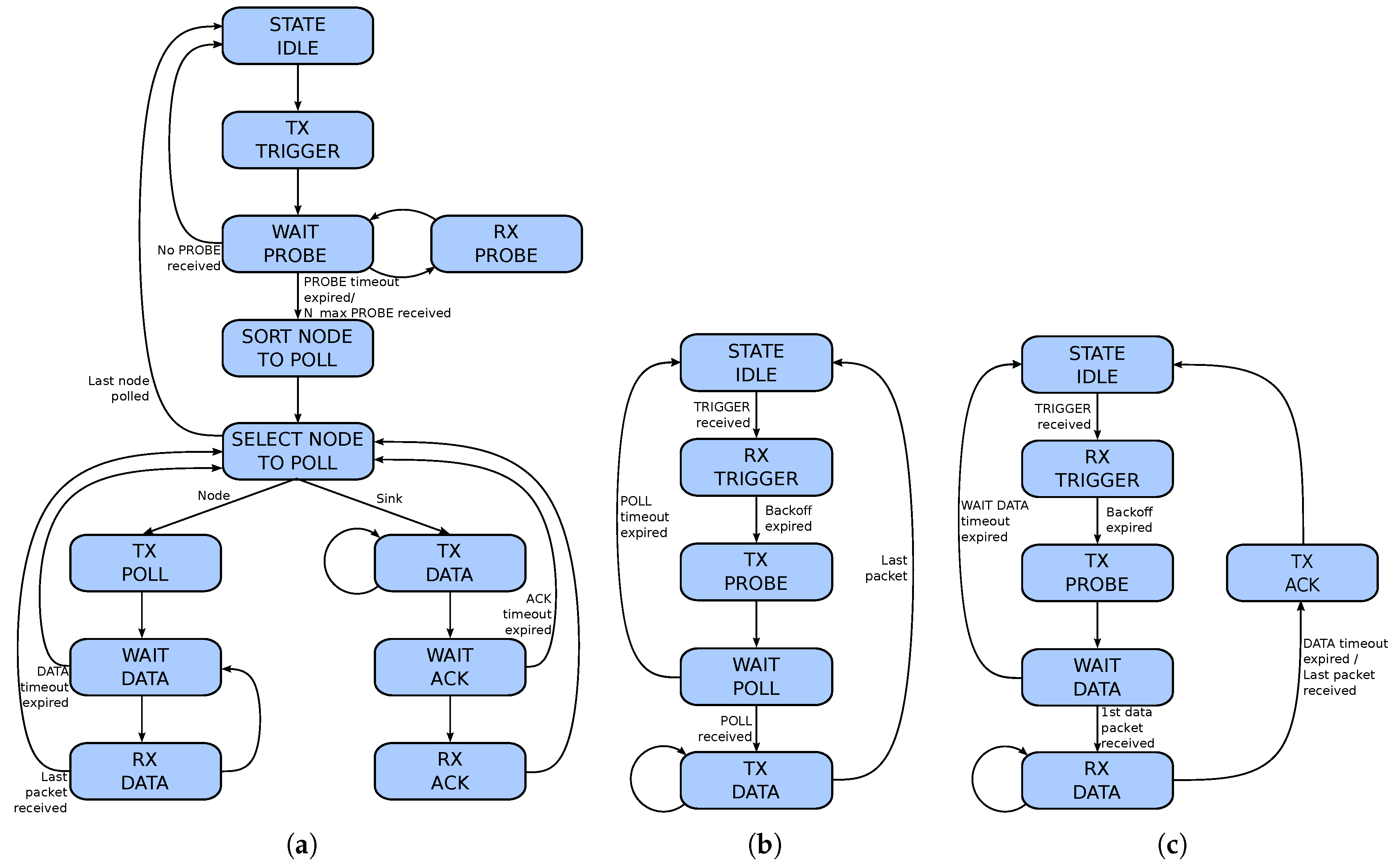
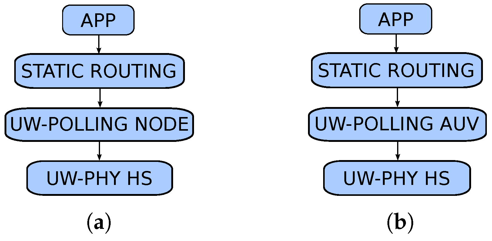
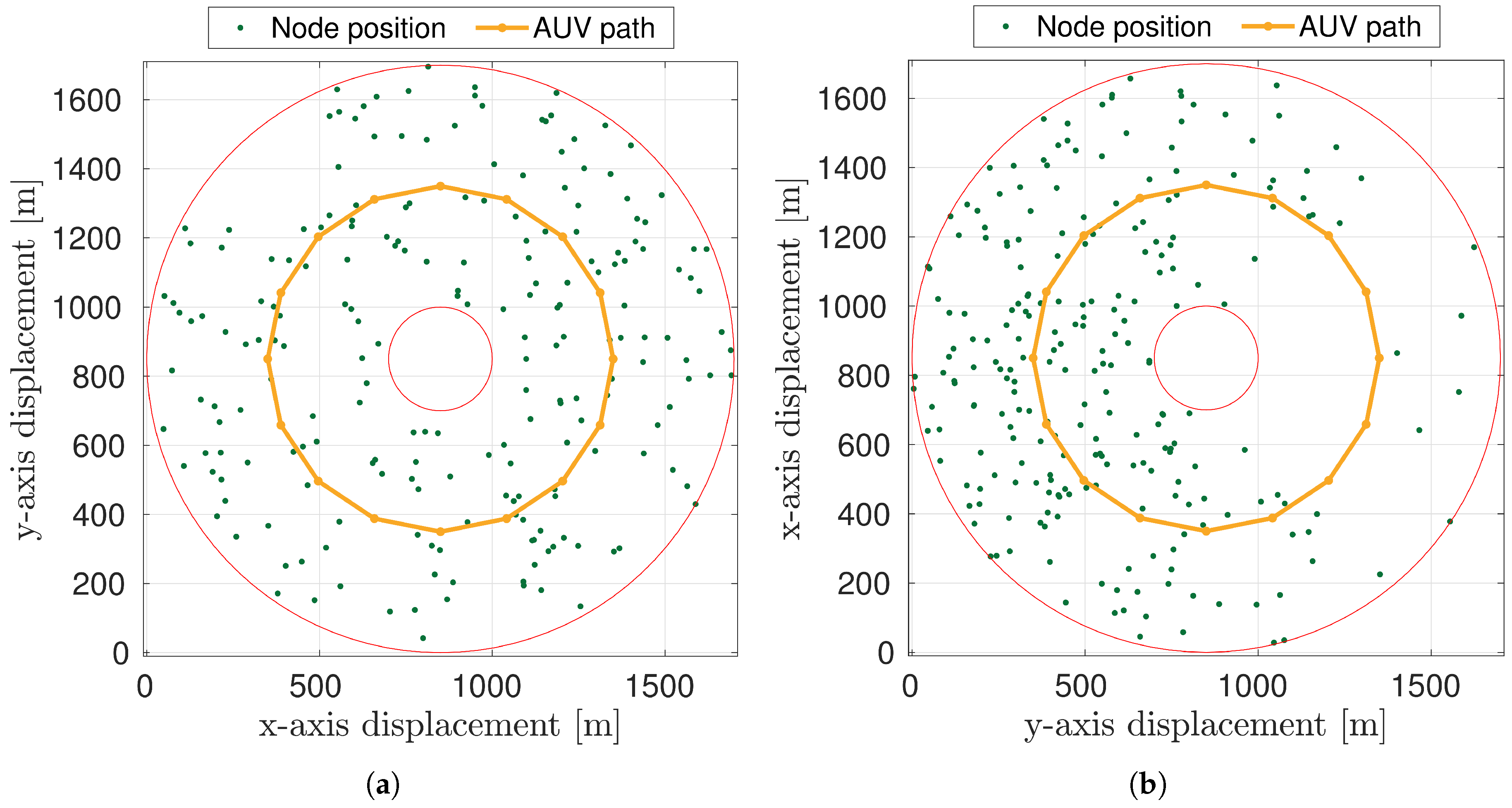


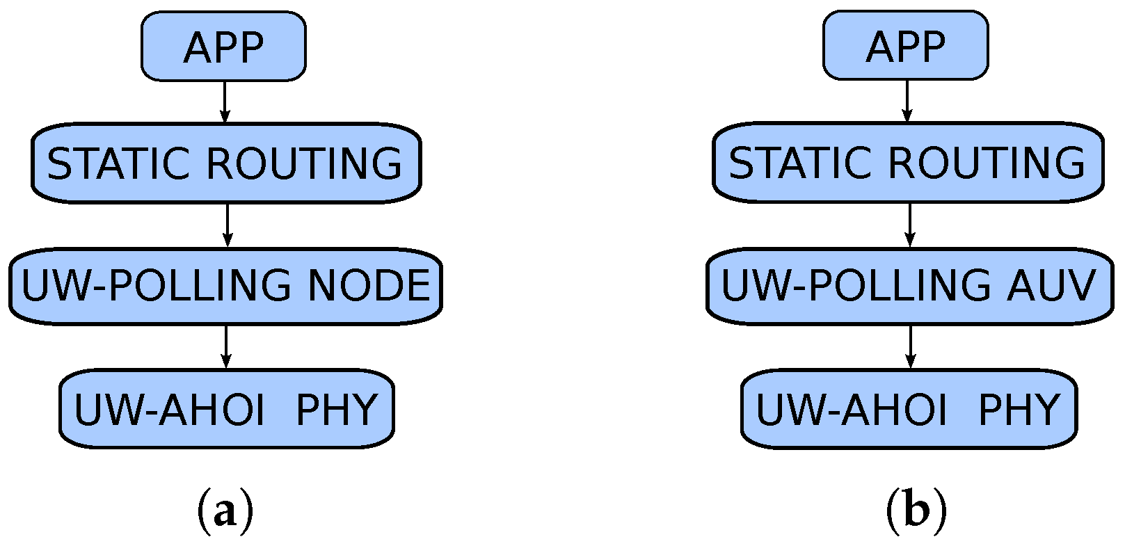


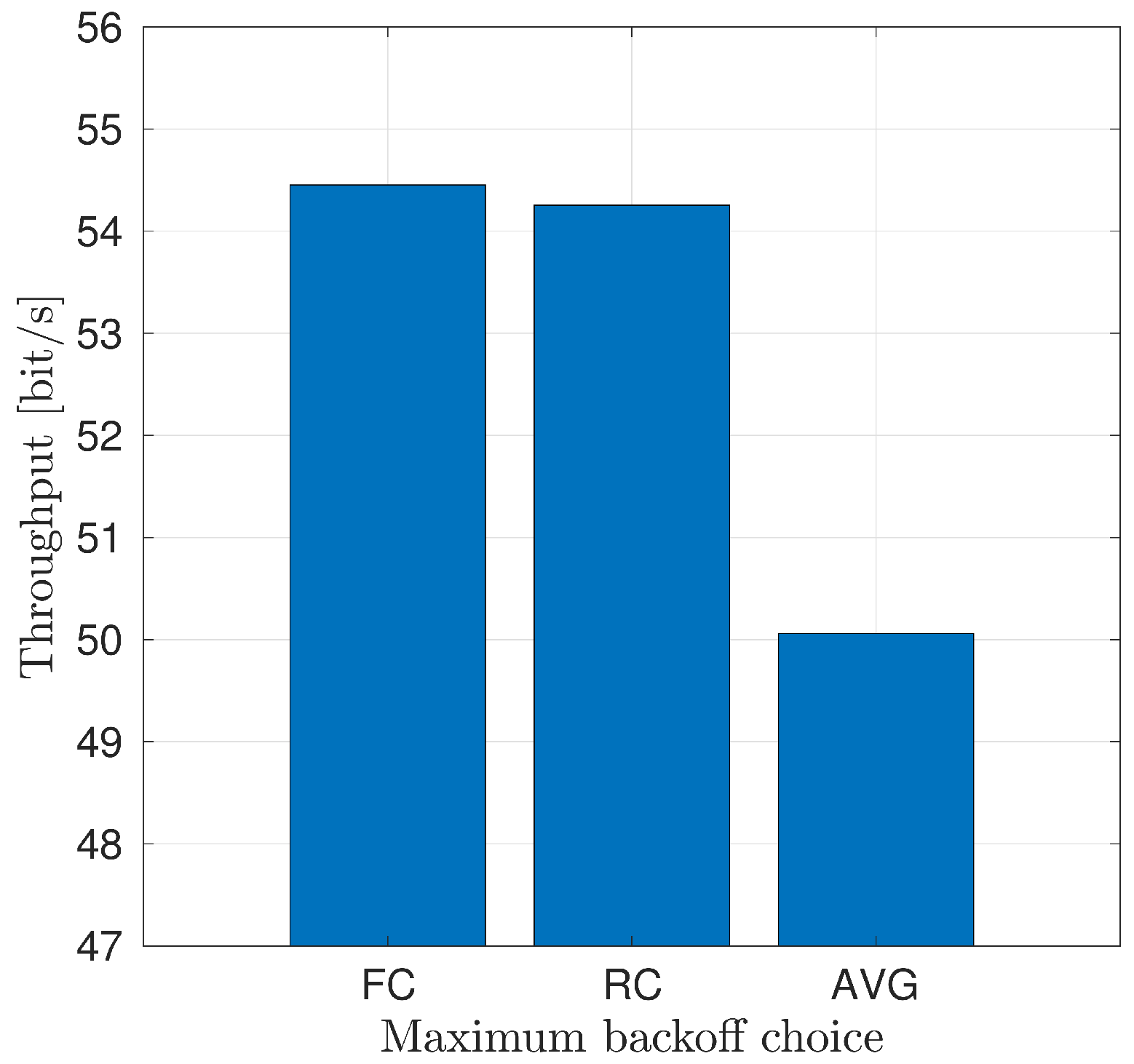
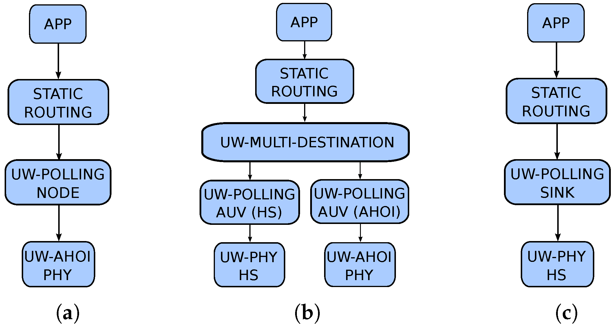

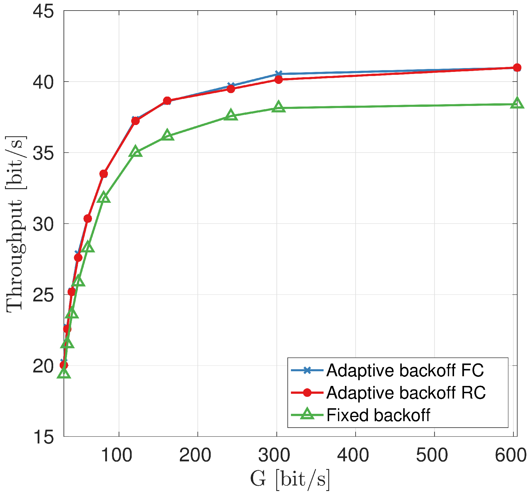
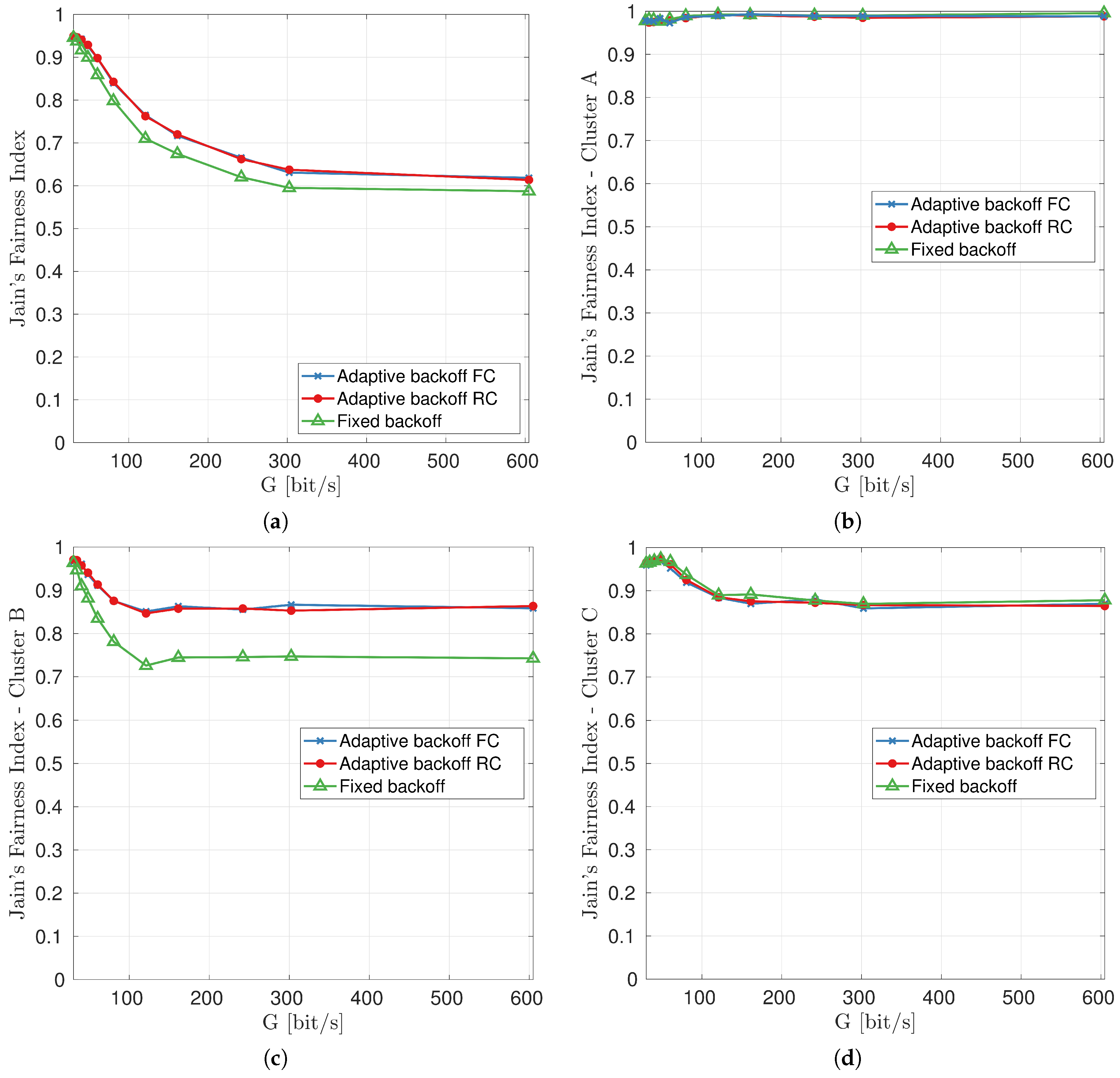
© 2019 by the authors. Licensee MDPI, Basel, Switzerland. This article is an open access article distributed under the terms and conditions of the Creative Commons Attribution (CC BY) license (http://creativecommons.org/licenses/by/4.0/).