Data Imputation in Wireless Sensor Networks Using a Machine Learning-Based Virtual Sensor

Abstract

Data integrity in wireless sensor networks (WSN) is very important because incorrect or missing values could result in the system making suboptimal or catastrophic decisions. Data imputation allows for a system to counteract the effect of data loss by substituting faulty or missing sensor values with system-defined virtual values. This paper proposes a virtual sensor system that uses multi-layer perceptrons (MLP) to impute sensor values in a WSN. The MLP was trained using a genetic algorithm which efficiently reached an optimal solution for each sensor node. The system was able to successfully identify and replace physical sensor nodes that were disconnected from the network with corresponding virtual sensors. The virtual sensors imputed values with very high accuracies when compared to the physical sensor values.

1. Introduction

Wireless sensor networks (WSN) gained popularity in recent years as the world embraces Internet of Things (IoT) applications as part of the 4th industrial revolution [1,2,3,4]. The sensors in WSN applications are used to gather data about the environment and these nodes communicate with each other and possibly a base station in order to collaboratively monitor the application environment and make “intelligent” decision in reaction to the sensed condition [5]. A problem arises in WSNs, where due to the nature of these devices, data can be lost or corrupted during the transmission phase due to external interference in the communication line or malfunction sensors which produce faulty unreliable data [6]. Furthermore, the cost of implementing or needing to replace many physical sensors in a network can become prohibitively expensive.

The integrity of received information is an important issue in the modern age. Sensors play a pivotal role in electronic devices of all shapes, sizes and function and especially more so in WSNs where data loss is an expected occurrence [7]. The integrity of the data in WSN is not only an issue with regards to the naturally occurring external factors, there are also sinister threats to these vulnerable devices. The practical limitations of these devices mean that they are vulnerable to security attacks from people with malicious intent [8]. This means that an attacker may be able to seize control of one or more sensor nodes and alter the data in order to manipulate the system into making potentially disastrous decisions which could negatively affect the application environment [9].

In network security, there is a heavy emphasis on preventative security mechanisms which provide an external security perimeter to prevent an attacker from gaining access to the system [10]. When these preventative security mechanisms fail, detection mechanisms, diversionary tactics and countermeasures can be used to limit the potential damage an attacker can cause [11]. Intrusion Detection and Prevention Systems (IDPS) can thus be used in WSNs to detect and limit the damage of successful attacks by for example disregarding sensor readings from suspicious nodes [12]. Another important research focus is the detection of the location of the malicious node which is not trivial in the resource constrained environments [13,14,15]. This is because these countermeasures may affect the limited system resources which are required by the main application.

Data imputation is a method that allows a system to counteract the effect of data loss by accurately substituting values that real sensors would most likely have returned [16]. This then allows the system to still make use of incomplete data rather than completely discarding affected data entries. In the previous example this means that the IDPS would be able to disregard the suspicious sensor readings without significantly affecting the system’s performance. The focus on this paper is not on the detection of intrusions, but rather on a possible countermeasure that can be used once an attack has been successfully detected. This countermeasure can also be used when a node is disconnected from a system or has faulty readings in non-malicious circumstances. Data imputation is also traditionally used to replace missing/faulty sensor values at particular time instances. This is possible when the previous values of the affected sensor are used to infer what the current value should be. For algorithms that use the other sensor values to infer what the affect sensor value should be, it is necessary to have a separate imputation/filtering technique to infer values at specific time-instances. This is because these algorithms require the remaining sensor values to be accurate in order to effectively infer the missing values. These types of algorithms are more suitable as virtual sensor, which replace the affected sensor values for a specified time period instead of only at specific time instances.

Traditionally statistical techniques were the preferred choice to impute data but in recent years machine learning has been increasingly applied to the field [17,18,19]. These machine learning techniques have been proven to be more accurate and robust than their statistical counterparts [19]. K-Nearest Neighbours (KNN: lazy learning) [20], multi-layered perceptrons (MLP: supervised learning) [21] and self-organizing maps (SOM: unsupervised learning) [22] are three popular machine learning methods that have been used to great effect to solve the missing data problem in various applications. These algorithms were all able to outperform the traditional imputations techniques such as hot-swapping by significant margins in applications such as breast cancer detection, seed classification and sonar imaging. Most of the published work in this regard is on data mining techniques on incomplete datasets while the proposed work focuses on the real-time imputation of sensor values in resource constrained WSNs. This is important because sensor nodes are both vulnerable to security attacks and also prone to random non-malicious failures [23]. It is not always possible to expeditiously thwart a security attack or replace faulty nodes so a temporary solution is required. The proposed solutions should not have a large enough overhead to interfere with main application of the WSN as that would render them infeasible in practice. The resource limitations of these systems however make this challenging because traditional network security approaches are mostly not applicable in this setting [24].

This paper proposes the use of data imputation methods and machine learning in WSNs to realise virtual sensors. These virtual sensors are able to completely replace physical sensor nodes and give accurate substituted data in place of nodes with failed sensor modules. A Kalman Filter is used for the imputation of missing/faulty sensor readings at particular time instances and a Multilayer Perception is used to infer the virtual sensor values. The former was necessary due to the error prone sensor readings and anomalous environmental conditions which could affect the virtual sensor predictions. The main function of the proposed system is to ensure the robustness of WSNs by ensuring that damaged or compromised nodes in these systems can be replaced by these machine learning-based virtual sensors. This intervention reduces the effects, on system performance, of not being able to use the sensor data from the affected nodes. This allows the system to continue operating with little to no effect while using imputed values that closely resemble the affected sensor nodes’ would-be data.

The rest of this paper is organised as follows: Section 2 gives a brief background of all the relevant topics while Section 3 broadly describes the proposed system. The detailed design of the system is outlined in Section 4 and the results are presented and discussed in Section 5 and Section 6 respectively. Finally, the paper is concluded in Section 7.

2. Background

Much of the research based on virtual sensors has focused on using different machine learning approaches in representing the lost data or in creating new data by finding the relationship between different nodes in a network [25,26,27]. Virtual sensor systems implementing machine learning can be segmented into three main different types of learning namely lazy learning, supervised learning and unsupervised learning.

2.1. Learning Systems

In model-based data imputation machine learning applications, the data is used to train a model that finds a relationship between the inputs and outputs and the model is used to predict a value that can replace the missing values. In lazy learning systems, there is no prediction model so all relevant data points have to be searched to find the closest matching neighbours to the incoming inputs each time a query is made. Once the nearest neighbours are found the data can be imputed using statistical parameters such as the mean or standard deviation or indeed model-based machine learning algorithms [28]. The k-Nearest Neighbours (KNN) algorithm [29] is one of the most widely used methods in this category. As the name implies, the algorithm attempts to find the k nearest neighbours to the data instance that is being used for classification or regression. Several different measures can be used to determine the degree of proximity [30] with the most popular being the Minkowski distance for imputation applications. Once the nearest neighbours are determined, the imputed value will be classified as part the majority category for classification problems. If it is a regression problem, the weighted average output of the neighbours will be used as the imputed value. The advantage of these systems is that their simplicity and relatively high accuracy while the drawbacks are the computational complexity and inefficiencies when dealing with categorical data. Zhang [28] however proposed a variant of kNN that uses gray relational analysis to evaluate the degree of proximity which worked well for both numeric and categorical variables. This method outperformed other kNN state-of-the-art techniques based on the popular Minkowski distance. The accuracy of these systems is heavily reliant on the selection of an optimal K-value, the distance metric and the imputation technique used. The resource constraints of the WSN application environment [31] means that this category of algorithms will not always feasible in practice.

In supervised learning systems, unlike the lazy learning systems, the algorithm requires a training phase to generalise data in the form of a model that can be used to impute missing values. Learning is supervised in the manner that training targets are provided to the algorithm for the desired model and parameters are adjusted accordingly over many training epoch cycles until a desirable model emerges. One of the most popular of these supervised learning systems is the artificial neural network (ANN) [32]. Multiple layered perceptrons (MLP) [33] are a form of feed-forward neural networks (FFNN) which have a basic structure consists of several interconnected artificial neurons or nodes that can be categorised into three main layers depending on their location in the network. The network has one input layer which has a node count that is equivalent to the number of inputs. The network also has at least one hidden layer but can more layers depending on the complexity of the problem. Finally, the network has an output layer which has the same number of nodes as the number of outputs. MLPs are universal function approximators which allow them to create mathematical models through regression analysis as well as being useful in the field of classification problems. In this category of algorithms it is generally the case that the more training data available, the more accurate the model will be. This is especially the case in deep learning applications which could require more complex networks and larger training datasets. Iwashita et al. [34], for example, successfully used a convolutional neural network to impute thermal image data from conventional RGB images.

In unsupervised learning systems, the algorithm requires a training phase but, unlike supervised learning systems, the system does not use the input/output relationship of the data to find the model representation. This means that the algorithm is taught how the data is structured instead of how to map the input/output relationship of the data. The Kohonen map [35], otherwise known as a SOM, is a widely used type of FFNN with an input layer and an output layer each of which has multiple nodes associated with the layer. The goal of the SOM is to organise the neural network outputs in such a manner that the target data is mapped accurately. The algorithm makes use of competitive unsupervised learning where the neurons compete using the Euclidian distance between the input vectors and their own vectors to find the closest match [22]. The weights are then iteratively adjusted accordingly until an optimal solution is found. In data imputation applications these algorithms have been found to be accurate and robust although they are more resource-intensive than MLPs. Folguera et al. [36] were able to show the effectiveness of this approach by predicting physicochemical water parameters. The algorithm had comparable results to imputations made by experts through inference.

2.2. Virtual Sensor

A virtual or soft sensor is a digitised emulation of a physical sensor node. There are two main types of virtual sensors, those that obtain sensor values from underlying physical devices [37] and those that infer the values based on other physical parameters [38]. The former is ideal for cloud-based applications where users are able to remotely access live sensor readings and parameters without worrying about the configuration and maintenance of the WSN. The latter type of virtual sensor is used to impute sensor readings from unreliable or compromised nodes so as not to affect the performance of the system.

The authors in [39] proposed a virtual sensor based on the recurrent neural network (RNN) that replaces the time-series values of a broken wave sensor with the imputed values. The proposed system is made more efficient by making use of the piecewise approximate aggregation algorithm for dimensionality reduction. The imputed sensor values produced a small enough error to enable the system to continue functioning optimally even when the broken wave sensor readings were replaced.

The authors in [40] proposed a virtual sensor management system that allows users to set their quality of service parameter. Sensor readings which fall below the selected threshold are disregarded and replaced with imputed values using the association rule mining technique. In this scenario the virtualisation of the sensors is part of the first category of virtual sensors (i.e., the physical devices are still operational) and the sensor values are only imputed if they are missing or fall below the quality control threshold. The proposed system was able to produce promising results when compared to state-of-the-art imputation techniques. Both scenarios illustrate that the virtualisation of sensor nodes is able to limit the impact of unreliable or faulty sensor readings on system performance.

3. System Overview

This paper is largely concerned with the identification of the relationship between sensor nodes in a sensor network using data that has been collected by the sensor network hence many of the above algorithms are applicable to the proposed scenario. Multiple temperature sensor nodes were deployed to generate training data resulted and each sensor node had a corresponding virtual sensor. A FFNN was used to model the relationship between the deployed sensor nodes in the network and these models were used to create the virtual sensors. For training, a genetic algorithm (GA) was chosen due to experimental evidence showing that the training method converges much faster than the back-propagation algorithm [41]. This reduces the required training time as well as the likelihood of falling into the potential trap of local optimums which may require a reinitialisation of the training due to stagnant results.

A star topology was chosen for the sensor network that would make use of WiFi communication technology where the sensor nodes would communicate with a central server. Low power usage is of no concern in this paper where the primary concern is with sensor networks where distances from each node are not too far apart from each other (<50 m) which would mean that expensive technology such as ZigBee and LoRa are not required. The database of the system will be stored locally by the server and used as training and test data for the VS once enough data has been gathered. A separate database will collect the VS outputs for comparison to real sensed data once training is complete. Figure 1 shows the conceptual design of the proposed system.

3.1. PhysicalSensor Nodes

The ambient temperature where the sensor nodes would be deployed was not expected to change abruptly under normal conditions so a sampling rate of one sample per 30-s interval was chosen. No scaling circuit was designed as the modified Steinhart-Hart equation [42] was deemed a better software solution than using hardware to convert the sensed values to corresponding temperatures. A filtering algorithm was required to account for the noise that was experienced. This noise was due to temperature anomalies as a result of hot air pockets moving through the buildings as well as hardware glitches. A scalar Kalman filter (SKF) was designed and implemented in software on the server to deal with these anomalies as it was accurate as well as being computationally simple.

3.2. Virtual Sensor

For the virtual sensor, a supervised MLP algorithm was used to find a model representation of the relationship between the deployed sensors. An algorithm was implemented to iterate through various topologies based on several hidden nodes as well as hidden layers to determine an optimal middle ground where an acceptable accuracy was reached by the MLP while taking training time into consideration. During Training the fittest neural networks are selected for breeding using the GA. Parents are then randomly selected for breeding, irrespective of which parent is the fittest in the subset population. Weights are randomly selected across both parents’ weight arrays to complete a child neural network’s weight array with a small chance to completely randomise a single weight in the array to act as a mutator until the original population size is reached. This is repeated over a specified number of epochs until a candidate neural network emerges for a specific VS.

The VSs are deployed on both the server and the sensor nodes, applying the weights that have been found through the training phase. The system will identify if a sensor node is not communicating with the server and use the appropriate VS to take over sensing operations until the sensor node is able to reconnect to the network. If this is not the case, the sensor node will send both VS data and physically sensed data back to the server.

4. System Design

4.1. Sensor Node

The sensor circuit is implemented using an NTC thermistor to realise a temperature sensor and the PIC32MX220F032B (PIC32) microcontroller as the processor unit. Two voltage divider circuits were implemented with the outputs connected to different analog input pins on the microcontroller meaning two temperature sensors were implemented per sensor node. This was done for redundancy since components may have slightly different tolerances than specified in the datasheet.

For the wireless communication there was a choice between using Bluetooth technology or WiFi. WiFi was chosen as TCP/IP was the preferred method of message transmission in the network and the chosen star network topology. The ESP8266 WiFi module was chosen due to the low power options available on the ESP8266 microcontroller as well as for the ability to communicate through USART. Four ESP8266 WiFi modules were implemented in the paper, one to serve as the server’s communication device and the other three to be used on each sensor node. Each node needs to establish a connection with a server which requests sensor readings from all three nodes every 30 s. Should the connection between the node and server be unreliable/interrupted, the values are replaced by the virtual sensor readings until it is able to establish a reliable connection with the server.

The client communication modules which act as the client’s communication interface, require communication through USART to transmit all received data to the microcontroller as well as transmit data over WiFi when data is received through USART from the microcontroller. These modules communicate with the server communication module which acts as the server’s communication interface requires communication through USB to transmit all received data to the server on the desktop PC. To enable this communication a serial-to-TTL device was required. The schematic of the sensor node is shown in Figure 2.

4.2. Scalar Kalman Filter

During experimentation it was found that there is a rare glitch in the system that occurs when a sensor node reconnects to the network where ground values are received instead of the expected sensor readings. An SKF was designed and implemented to filter out the glitches as well as to smooth out the received readings. Equation (1) shows the five equations that make up the SKF where x is the sensor reading, S is the prediction, M is the prediction error, K is the Kalman gain, and ${\sigma }_u$ is the noise covariance. The noise analysis of the SKF was done using gathered data and scaling up the noise covariance. The functional flow of the SKF is shown in Figure 3. The covariance noise value was determined and chosen to be 0.01 which resulted in minimal loss of data was experienced and the glitches were successfully filtered out. As can be seen in Figure 4 the overall shape of the graph does not vary as much from the original while still being able to filter out the glitches more effectively than smaller or larger Q values.

$$\begin{array}{cc}\hfill Prediction:S\left[n\right|n-1]& =aS[n-1|n-1],\hfill \\ \hfill Predictionerror:M\left[n\right|n-1]& ={\sigma }_u^2+a^{2}M\left[n\right|n-1],\hfill \\ \hfill Kalmangain:K\left[n\right]& =\frac{M\left[n\right|-1]}{{\sigma }_n^2+M\left[n\right|n-1]},\hfill \\ \hfill Correction:S\left[n\right|n]& =S\left[n\right|n-1]+K[n\left]\right(x\left[n\right]-S\left[n\right|n-1\left]\right),\hfill \\ \hfill Updateerror:M\left[n\right|n]& =(1-K[n\left]\right)M\left[n\right|n-1]\hfill \end{array}$$

(1)

4.3. Data Imputation

4.3.1. Neural Network Structure

The MLP neural network was the chosen algorithm to implement the virtual sensor in the WSN. A topology of three input nodes, eleven hidden nodes plus bias node and one output node was chosen. The number of input and output nodes correspond to the number of system inputs and outputs respectively. A configuration with only three sensors was selected to increase the complexity of the problem. The more sensors the system had the easier it would have be to impute missing/incorrect values using the remaining sensors. In this case, the input values are the other two sensor readings and the third input is the time of day the readings were taken. There is only one output because the idea is that each MLP should be able to predict the value of one faulty sensor using the other two sensors which are presumably functioning correctly. Several different hidden layer configurations were evaluated the one that produced the best results only had one hidden layer with eleven neurons. Having multiple hidden layers with a smaller number of neurons in each layer increased the training time considerably while not getting significantly better results than the chosen configuration. It was thus decided to have one hidden layer where the evaluated number of nodes in the layer were between three and twelve over 500 epochs. The chosen configuration was preferred because it has a fast training time and does not overfit the data while also not being too computationally expensive. The output can be described mathematically as the sum and products of the inputs, weights and activation functions. Equation (2) shows how the output of each input layer hidden layer is calculated where $x_{1,i}$ is the normalised input to the input node.

$$a_{1,i}=\frac{x_{1,i}}{1+\left|x_{1,i}\right|}$$

(2)

The output of each hidden layer is shown in Equation (3) where $x_{2,i}$ is the result of the sums of the inputs multiplied by the weights (Equation (4)). Finally, Equation (5) shows the output layer which uses a linear activation function.

$$a_{2,i}=\frac{x_{2,i}}{1+\left|x_{2,i}\right|}$$

(3)

$$x_{2,i}=\sum _{i=1}^N\sum _{j=1}^3{w}_{i,j}·a_{1,i}$$

(4)

$$a_3=\sum _{i=1}^N{w}_i·a_{2,i}$$

(5)

In addition to the above, the input layer and every hidden layer has a bias node included that is not connected to the previous layer. This is implemented to increase the flexibility of the model to fit the data and to allow the network to fit data if in the unlikely scenario all the input features are equal to zero.

4.3.2. Genetic Algorithm

Genetic algorithms (GA) are based on the principle of natural selection and form part of the broader field of evolutionary computation [43]. Analogous to its biological counterpart the idea behind evolutionary computing is to search the multiple different possibilities to find an optimal solution. In biology, the genetic sequences most likely to be passed on to the next generations are the ones which will most likely allow them to survive in harsh environments to ensure the survival of the species. In evolutionary computation, only the solutions which are the most effective in solving the problem are allowed to “reproduce” until an optimal solution is found. In both cases evolution is spurred on by random variation and then a process of “natural selection” evaluates each of these variations to find the best candidates to be passed on to the next generation.

A genetic algorithm was designed and implemented for neuro-evolution of the MLP as shown in Figure 5. There are four main steps involved in using the genetic algorithm to train the MLP, namely the forward propagation, prediction, error calculation, parent selection and finally repopulation. GA’s start by initialising a random population of chromosomes (i.e., solutions) which consist of several genes (i.e., sub-solutions) in particular loci (i.e., positions) within the chromosomes and represent instances of alleles (i.e., traits). In MLPs, GAs generally use the weights as the genes but there are other implementations that combine the weights as well as the number of nodes and hidden layers. This means that the first step is to initialise a population of MLPs with random weights. Once the weights initialised the MLPs can predict the sensor values by forward-propagating through the networks as described by Equations (2)–(5). Each prediction is based on three input parameters which are the other two sensor node inputs in the WSN and the time that those data points were collected during the day. The output of the forward propagation stage is the predicted virtual sensor value which will not be very accurate during this initial step.

The error of each MLP prediction is then calculated using based on some pre-determined error function. For this application the mean absolute error (MAE) is used as shown in Equation (6) where $p_i$ is the value predicted by the MLP, $t_i$ is the target value associated with the inputs, and N is the number of training points. Genetic algorithms are structured such that the strongest members of the population will have a high probability of reproduction while the weakest members will not have good chances of surviving the selection process. This means that the genes of offspring will likely be made up of combinations of the genes of the strongest chromosomes from the previous population. In this application the selection of parent MLPs is done immediately after the last MLP in the population has had its MAE calculated after forward-propagating through the entire training dataset. The parent population is chosen as the top 10% of the entire population and these will be used to breed the next generation of MLPs. Breeding parents are selected at random from this population without regard for which have strongest solutions.

$$MAE=\frac{{\sum }_{i=1}^N\left|p_i-t_i\right|}{N}$$

(6)

Reproduction (or crossover) occurs when the genes of two chromosomes (called parents) are mixed to produce new chromosomes (called offspring). A process of mutation, in which genes are altered to represent different alleles is also applied to a subset of offspring to replicate the copying error induced mutations of their biological counterparts. These offspring and their mutations will then be evaluated as part of the new population and only the strongest members of that population will be allowed to reproduce. The crossover and mutation processes do not use fixed parameters but rather rely on probabilities. The former is called the crossover rate and is a measure of the chances of a crossover occurring at a particular point. The probability that a gene is copied over to the child MLP is calculated using the error associated with both parents using Equation (7). In the equation, $MA{E}_n$ is the error associated with each parent. This allows the fitter parent a higher likelihood of transferring weights that are more desirable. The mutation rate is the probability of a mutation happening at each lotus after the crossover process. There is a chance that none of the genes of a particular offspring will be mutated as this is heavily dependant on the chosen rate.

$$P\left(A\right)=1-\frac{MA{E}_1}{MA{E}_1+MA{E}_2}$$

(7)

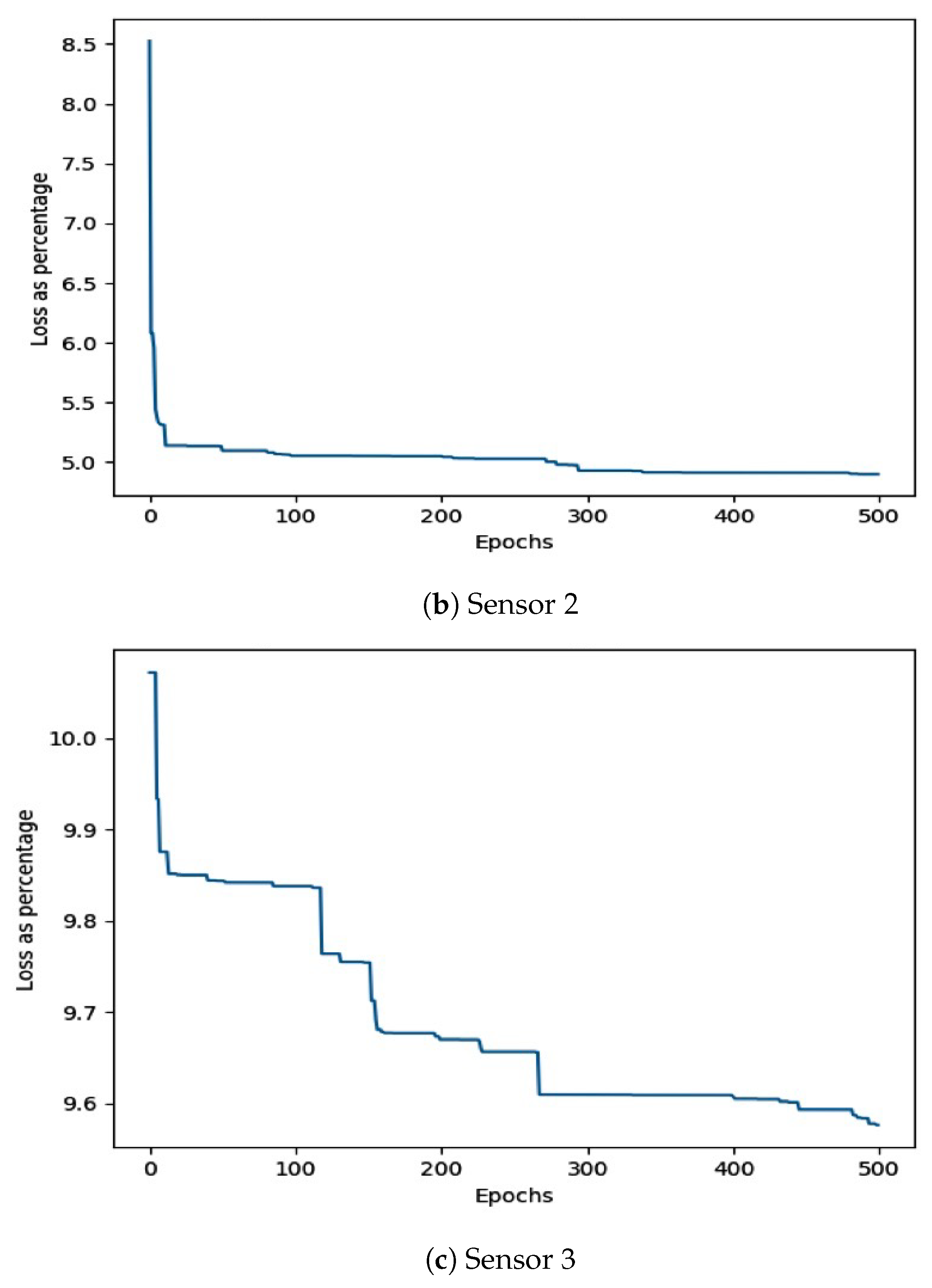
To avoid stagnation in the population as the training epochs increase, every gene, when copied, has a small probability (<=2%), to be completely randomised instead of copied over from the parent MLPs. This ensures that there is always some diversity in the genetic pool of the MLP population. This evolutionary process typically continues until it produces an optimal solution. In the application environment the process is repeated beginning with the forward propagation step until the specified epoch number has been reached. Specifying the optimal number of epochs is thus very important because if this value is too small an optimal solution will not be found but if it is too large it could lead to overfitting. For this application the training loss was simulated over 500 epochs for each sensor node and the results are shown in Figure 6.

5. Results

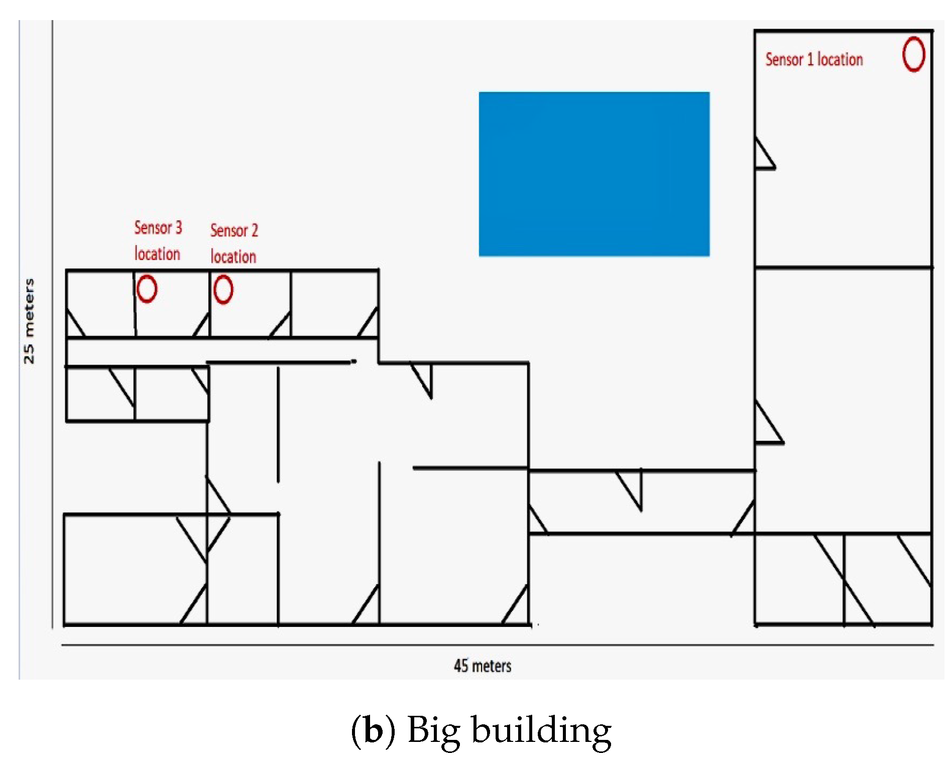
To test the performance of the proposed system it was deployed in 2 different scenarios as shown in Figure 7.

5.1. Virtual Sensor Accuracy

An experiment was carried out to test the accuracy of the virtual sensor imputation values. The analysis was performed using 14,000 VS and physical sensor readings acquired from the experimental setup over a five-day period. Then physical sensor readings were considered the ground-truth when acquiring the accuracy percentage for the VS. The sensor readings were saved onto a dataset and the accuracy is evaluated offline for convenience. The system contains three virtual sensors, one for each physical sensor, and each of them are evaluated independently. For VS1, physical sensors 2 and 3 (and the timestamp) are used to predict the values of physical sensor 1. The accuracy of the prediction is then found using Equation (8). The process continues for each time instance until all 14,000 data points have been evaluated. Once completed the minimum, maximum and average accuracy for the VS values can be calculated and the system evaluated. VSs 2 and 3 go through the same process so that there are three independent accuracy metrics for each VS. In this way the system is able to simulate what would happen if the physical sensor values had to be imputed and evaluate how accurate the imputed values will be. The results of the experiment are shown in

Table 1. Accuracy results of the deployed virtual sensors.

Building	VS #	Min acc %	Max acc %	Avg acc %
	VS 1	78.96847	99.99847	94.03248
Small	VS 2	92.47204	99.99996	97.07589
	VS 3	86.52291	99.99825	95.15422
	VS 1	85.52389	99.99967	94.70205
Large	VS 2	88.34544	99.99998	96.54874
	VS 3	87.90576	99.99992	96.28131

.

$$acc=(1-\frac{|V{S}_i-senso{r}_i|}{senso{r}_i}\times 100)$$

(8)

The minimum, maximum and average accuracy expressed in percentages were recorded for each virtual sensor using both acquired datasets. The overall averages of the small residential building virtual sensors were around 95%. The overall averages of the large residential building virtual sensors also had similar performance. The worst-case accuracy experienced was by virtual sensor 1 in both cases with 78.97% and 85.52%. The best-case scenario resulted in a near 100% accuracy for all three sensors in both test cases. This means that the system is accurately able to model the relationship between the 3 sensors.

Comparison with State-of-the-Art

To adequately evaluate how well the system works it was compared to the performance of other state-of-the-art techniques. The two techniques chosen in this regard are kNN and linear regression. The former is a typical data-mining used to impute missing values in large datasets. The latter is a typical statistical approach the models the input out relationship of the system to deduce future values. These techniques were chosen to represent the aforementioned algorithm types in the application environment. The results of the experiment are shown in

Table 2. Accuracy of the deployed virtual sensors vs state-of-the-art techniques.

Building	VS #	MLP %	kNN %	LinReg %
	VS 1	94.03248	91.34519	91.80413
Small	VS 2	97.07589	92.55777	93.88260
	VS 3	95.15422	81.60299	79.39729
	VS 1	94.70205	78.94263	71.84740
Large	VS 2	96.54874	85.37011	86.25564
	VS 3	96.28131	81.38311	81.31372

.

In the small building the results of all of the algorithms are comparable except when looking at VS3. This is because sensor 3 is in a different environment when compared to the other two sensors. The result is that both kNN and linear regression struggle a lot more to predict this value accurately whereas the proposed scheme has little difference between the three sensors. This means that it is more robust than both kNN and linear regression. In the big building there is a significant disparity between the proposed scheme and the state-of-the-art techniques. The results of the proposed scheme are only slightly lower than they were in the small building but even in this case the results are comparable. There is also little difference in the results when looking at the sensor location within the building. Both kNN and linear regression have far lower accuracies in this configuration than they did in the small building. The latter struggles particularly to infer the value of VS1 because the sensor is in a vastly different environment when compared to the other two sensors. In general though, all three algorithms perform well in the application environment with the proposed scheme being the most accurate and robust of the three algorithms.

5.2. Standard Deviation

An experiment was carried out to calculate the standard deviation of the virtual sensor imputation values. The analysis was performed using 14,000 VS and physical sensor readings acquired from the experimental setup over a five-day period for the small building and a seven-day period for the bigger building. The sensor readings were considered the ground-truth when acquiring the errors for the VS. The standard deviation in °C is recorded in

Table 3. Standard deviation results of the deployed virtual sensors.

Building	VS #	STD DEV (°C)
	VS 1	1.226344
Small	VS 2	0.518652
	VS 3	0.721729
	VS 1	0.964535
Large	VS 2	0.784815
	VS 3	0.692576

the small and large residential buildings. The 5-day plots of the virtual sensor and physical sensor readings for the small residential building and the 7-day plots for the large residential building are displayed in Figure 8 and Figure 9 respectively.

5.3. Imputation Time

An experiment was set up to evaluate the time it takes to impute values on but the server and the physical sensor nodes. The time data is then averaged for each individual sensor over multiple iterations to get a mean-time-to-impute as well as the virtual sensors on the server. The minimum time and maximum time to impute is also extracted from the data. These results are shown in

Table 4. Virtual sensor time to impute.

Location	VS #	min (ms)	max (ms)	avg (ms)
	VS 1	382	588	413
Node	VS 2	391	547	412
	VS 3	378	550	412
	VS 1	9.322	9.366	9.379
Server	VS 2	9.343	9.392	9.379
	VS 3	9.327	9.374	9.379

.

6. Discussion

The success of any virtual sensor system using machine learning at the core of the design is dependent on the successful design and implementation of the chosen machine learning method as well as the quality of the training data that is used to train the virtual sensors. This was evident in the results obtained for the overall virtual sensor network and its associated subsystems. When the results for the accuracy are compared with regards to the size of a building it was found that a virtual sensor network deployed in a large residential building very marginally outperforms a small residential building, but this was negligible. It was further found that the system was able to impute values with an accuracy of around 95% for both deployed scenarios. The system was trained and evaluated using real sensor readings from the experimental setup described in the previous section. This means that the trained MLPs were deployed on the sensor nodes and could impute values in real time on the physical system. A more detailed discussion on the computational consideration will be deferred for later in this section.

When compared to state-of-the-art techniques it is evident that the proposed approach has better comparable results on average. Zhang [28] evaluated three kNN implementations on two popular datasets. The mean accuracy for all three algorithms on both datasets ranged from 85% in the worst case to 98% in the best case. As mentioned previously though, the approach proposed in this paper is more suitable for WSNs than kNN because of the resource constraints of the application environment. Folguera et al. [36] proposed and SOM technique for data imputation of physicochemical water parameters and compared it to data imputed by expert inference. The expert data yielded a mean accuracy of around 84% while the proposed SOM technique achieved a mean accuracy of almost 90%. The approach proposed in this paper is again preferred in the application environment because it is more resource friendly.

The choice of using genetic algorithms to train the MLP proved to be well suited in all three virtual sensor cases as evidenced by the standard deviation measurements in Table 3 and visualised by the plots shown in Figure 8 and Figure 9. It was seen that the virtual sensors accurately depicted the changes with very little variation between the measured and imputed temperatures values over several days.

It was found that with the increase in computational power in the modern-day has resulted in very fast turnaround times when imputing sensor values using an MLP. Even the 40 MHz processing speed of the PIC32 was able to impute values in under a second with the longest imputation lasting 0.588 s. On the server-side the desktop PC used for this system was able to impute values on average in 9.379 ms for all three sensors. Depending on the size and topology of the network, imputing the sensor values on the physical sensor node may not always be practical. In large networks where multiple sensor values have to be imputed an execution time of 0.588 s could cause significant delays which could affect overall system performance. The purpose of the proposed system is to maintain system performance even when some of the sensors are malfunctioning so if the proposed scheme also affects overall system performance it would be counterproductive.

The approach to implement the wireless communication in the WSN using WiFi communication was a positive design choice as many IoT applications in the literature make use of the TCP/IP stack which works well over the WiFi 2.4 GHz spectrum and allows easier management of clients that connect to the network. It was found that due to the power spikes that occur when transmitting data from the server that a query could only be sent every 5 s or WiFi module connected to the server would crash and require a cold restart which is due to the oscillations in current draw.

7. Conclusions

In this paper, a virtual sensor using machine learning was proposed for use in wireless sensor networks. The system was designed and implemented using an MLP neural network trained using a genetic algorithm. The genetic algorithm was able to converge on an optimal solution in a relatively small amount of time despite no parallelism being implemented into the training algorithm. A SKF was also designed and implemented to filter out noisy readings as well as to smooth out the received values. The SKF proved to be an effective filtering method in this application and could deal with anomalous values such as the ground glitches. In general, the system was able to successfully identify and replace a physical sensor node that was disconnected from the network with a virtual sensor. The virtual sensor imputed values with a very good accuracy when compared to the physical sensor values. For future work the algorithms ability to impute values of different sensor types in more complex application scenarios will be investigated. The number of sensors required in order to accurately impute values in dynamic and potentially non-linear environments will also be explored. Lastly, the use of multiple machine learning algorithms in combination (i.e., hybrid and ensemble schemes) to get possibly even more accurate virtual sensor results will also be investigated.

References

1. Kocakulak, M.; Butun, I. An overview of Wireless Sensor Networks towards internet of things. In Proceedings of the IEEE 7th Annual Computing and Communication Workshop and Conference (CCWC), Las Vegas, NV, USA, 9–11 January 2017; pp. 1–6. [Google Scholar]
2. Yaqoob, I.; Ahmed, E.; Hashem, I.A.T.; Ahmed, A.I.A.; Gani, A.; Imran, M.; Guizani, M. Internet of things architecture: Recent advances, taxonomy, requirements, and open challenges. IEEE Wirel. Commun. 2017, 24, 10–16. [Google Scholar] [CrossRef]
3. Sibanyoni, S.V.; Ramotsoela, D.T.; Silva, B.J.; Hancke, G.P. A 2-D Acoustic Source Localization System for Drones in Search and Rescue Missions. IEEE Sens. J. 2019, 19, 332–341. [Google Scholar] [CrossRef]
4. Nkomo, M.; Hancke, G.; Abu-Mahfouz, A.; Sinha, S.; Onumanyi, A. Overlay virtualized wireless sensor networks for application in industrial internet of things: A review. Sensors 2018, 18, 3215. [Google Scholar] [CrossRef] [PubMed] [Green Version]
5. Lu, W.; Gong, Y.; Liu, X.; Wu, J.; Peng, H. Collaborative energy and information transfer in green wireless sensor networks for smart cities. IEEE Trans. Ind. Inform. 2018, 14, 1585–1593. [Google Scholar] [CrossRef]
6. Peng, Y.; Qiao, W.; Qu, L.; Wang, J. Sensor fault detection and isolation for a wireless sensor network-based remote wind turbine condition monitoring system. IEEE Trans. Ind. Appl. 2018, 54, 1072–1079. [Google Scholar] [CrossRef]
7. Ramotsoela, D.T.; Hancke, G.P.; Abu-Mahfouz, A.M. A Survey of Anomaly Detection in Industrial Wireless Sensor Networks with Critical Water System Infrastructure as a Case Study. Sensors 2018, 18, 2491. [Google Scholar] [CrossRef] [Green Version]
8. Bhushan, B.; Sahoo, G. Recent advances in attacks, technical challenges, vulnerabilities and their countermeasures in wireless sensor networks. Wirel. Pers. Commun. 2018, 98, 2037–2077. [Google Scholar] [CrossRef]
9. Ramotsoela, D.T.; Hancke, G.P.; Abu-Mahfouz, A.M. Attack detection in water distribution systems using machine learning. Hum.-Centric Comput. Inf. Sci. 2019, 9, 13. [Google Scholar] [CrossRef]
10. Anwar, S.; Mohamad Zain, J.; Zolkipli, M.F.; Inayat, Z.; Khan, S.; Anthony, B.; Chang, V. From intrusion detection to an intrusion response system: Fundamentals, requirements, and future directions. Algorithms 2017, 10, 39. [Google Scholar] [CrossRef] [Green Version]
11. Inayat, Z.; Gani, A.; Anuar, N.B.; Anwar, S.; Khan, M.K. Cloud-based intrusion detection and response system: Open research issues, and solutions. Arab. J. Sci. Eng. 2017, 42, 399–423. [Google Scholar] [CrossRef]
12. Oke, J.T.; Agajo, J.; Nuhu, B.K.; Kolo, J.G.; Ajao, L. Two Layers Trust-Based Intrusion Prevention System for Wireless Sensor Networks. Adv. Electr. Electron. Eng. 2018, 1, 23–29. [Google Scholar]
13. Liu, X.; Liu, A.; Wang, T.; Ota, K.; Dong, M.; Liu, Y.; Cai, Z. Adaptive data and verified message disjoint security routing for gathering big data in energy harvesting networks. J. Parallel Distrib. Comput. 2020, 135, 140–155. [Google Scholar] [CrossRef]
14. Liu, Y.; Liu, A.; He, S. A novel joint logging and migrating traceback scheme for achieving low storage requirement and long lifetime in WSNs. AEU-Int. J. Electron. Commun. 2015, 69, 1464–1482. [Google Scholar] [CrossRef]
15. Liu, X.; Dong, M.; Ota, K.; Yang, L.T.; Liu, A. Trace malicious source to guarantee cyber security for mass monitor critical infrastructure. J. Comput. Syst. Sci. 2018, 98, 1–26. [Google Scholar] [CrossRef]
16. Jerez, J.M.; Molina, I.; García-Laencina, P.J.; Alba, E.; Ribelles, N.; Martín, M.; Franco, L. Missing data imputation using statistical and machine learning methods in a real breast cancer problem. Artif. Intell. Med. 2010, 50, 105–115. [Google Scholar] [CrossRef]
17. Sovilj, D.; Eirola, E.; Miche, Y.; Björk, K.M.; Nian, R.; Akusok, A.; Lendasse, A. Extreme learning machine for missing data using multiple imputations. Neurocomputing 2016, 174, 220–231. [Google Scholar] [CrossRef]
18. Duan, Y.; Lv, Y.; Liu, Y.L.; Wang, F.Y. An efficient realization of deep learning for traffic data imputation. Transp. Res. Part C Emerg. Technol. 2016, 72, 168–181. [Google Scholar] [CrossRef]
19. Liu, Y.; Gopalakrishnan, V. An overview and evaluation of recent machine learning imputation methods using cardiac imaging data. Data 2017, 2, 8. [Google Scholar] [CrossRef] [Green Version]
20. Dong, X.; Lin, L.; Zhang, R.; Zhao, Y.; Christiani, D.C.; Wei, Y.; Chen, F. TOBMI: Trans-omics block missing data imputation using a k-nearest neighbor weighted approach. Bioinformatics 2018, 35, 1278–1283. [Google Scholar] [CrossRef]
21. Verpoort, P.; MacDonald, P.; Conduit, G.J. Materials data validation and imputation with an artificial neural network. Comput. Mater. Sci. 2018, 147, 176–185. [Google Scholar] [CrossRef] [Green Version]
22. Wang, S. Application of self-organising maps for data mining with incomplete data sets. Neural Comput. Appl. 2003, 12, 42–48. [Google Scholar] [CrossRef]
23. Sen, J. A Survey on Wireless Sensor Network Security. Int. J. Commun. Netw. Inf. Secur. (IJCNIS) 2009, 1, 55–78. [Google Scholar]
24. Ramotsoela, T.D.; Hancke, G.P. Data aggregation using homomorphic encryption in wireless sensor networks. In Proceedings of the Information Security for South Africa (ISSA), Johannesburg, South Africa, 12–13 August 2015; pp. 1–8. [Google Scholar]
25. Oehmcke, S.; Zielinski, O.; Kramer, O. Input quality aware convolutional LSTM networks for virtual marine sensors. Neurocomputing 2018, 275, 2603–2615. [Google Scholar] [CrossRef]
26. Osman, M.S.; Abu-Mahfouz, A.M.; Page, P.R. A survey on data imputation techniques: Water distribution system as a use case. IEEE Access 2018, 6, 63279–63291. [Google Scholar] [CrossRef]
27. Salehi, H.; Das, S.; Chakrabartty, S.; Biswas, S.; Burgueño, R. A machine-learning approach for damage detection in aircraft structures using self-powered sensor data. In Proceedings of the SPIE Smart Structures and Materials + Nondestructive Evaluation and Health Monitoring, Portland, OR, USA, 25–29 March 2017; Volume 10168. [Google Scholar]
28. Zhang, S. Nearest neighbor selection for iteratively kNN imputation. J. Syst. Softw. 2012, 85, 2541–2552. [Google Scholar] [CrossRef]
29. Song, G.; Rochas, J.; Huet, F.; Magoules, F. Solutions for processing k nearest neighbor joins for massive data on mapreduce. In Proceedings of the 23rd Euromicro International Conference on Parallel, Distributed, and Network-Based Processing, Turku, Finland, 4–6 March 2015; pp. 279–287. [Google Scholar]
30. Walters-Williams, J.; Li, Y. Comparative study of distance functions for nearest neighbors. In Advanced Techniques in Computing Sciences and Software Engineering; Springer: Berlin/Heidelberg, Germany, 2010; pp. 79–84. [Google Scholar]
31. Sheng, Z.; Wang, H.; Yin, C.; Hu, X.; Yang, S.; Leung, V.C. Lightweight management of resource-constrained sensor devices in internet of things. IEEE Internet Things J. 2015, 2, 402–411. [Google Scholar] [CrossRef]
32. Tkáč, M.; Verner, R. Artificial neural networks in business: Two decades of research. Appl. Soft Comput. 2016, 38, 788–804. [Google Scholar] [CrossRef]
33. Ramchoun, H.; Idrissi, M.A.J.; Ghanou, Y.; Ettaouil, M. Multilayer Perceptron: Architecture Optimization and Training. Int. J. Interact. Multimed. Artif. Intell. 2016, 4, 26–30. [Google Scholar] [CrossRef]
34. Iwashita, Y.; Stoica, A.; Nakashima, K.; Kurazume, R.; Torresen, J. Virtual sensors determined through machine learning. In Proceedings of the World Automation Congress (WAC), Stevenson, WA, USA, 3–6 June 2018; pp. 1–5. [Google Scholar]
35. Singh, N.; Javeed, A.; Chhabra, S.; Kumar, P. Missing value imputation with unsupervised kohonen self organizing map. In Emerging Research in Computing, Information, Communication and Applications; Springer: Berlin/Heidelberg, Germany, 2015; pp. 61–76. [Google Scholar]
36. Folguera, L.; Zupan, J.; Cicerone, D.; Magallanes, J.F. Self-organizing maps for imputation of missing data in incomplete data matrices. Chemom. Intell. Lab. Syst. 2015, 143, 146–151. [Google Scholar] [CrossRef]
37. Madria, S.; Kumar, V.; Dalvi, R. Sensor cloud: A cloud of virtual sensors. IEEE Softw. 2014, 31, 70–77. [Google Scholar] [CrossRef]
38. Rallo, R.; Ferré-Giné, J.; Giralt, F. Best feature selection and data completion for the design of soft neural sensors. In Proceedings of the AIChE 2003, 2nd Topical Conference on Sensors, San Francisco, CA, USA, 16–21 November 2003. [Google Scholar]
39. Oehmcke, S.; Zielinski, O.; Kramer, O. Recurrent neural networks and exponential PAA for virtual marine sensors. In Proceedings of the International Joint Conference on Neural Networks (IJCNN), Anchorage, AK, USA, 14–19 May 2017; pp. 4459–4466. [Google Scholar]
40. D’Aniello, G.; Gaeta, M.; Hong, T.P. Effective quality-aware sensor data management. IEEE Trans. Emerg. Top. Comput. Intell. 2018, 2, 65–77. [Google Scholar] [CrossRef]
41. Siddique, M.; Tokhi, M. Training neural networks: Backpropagation vs. genetic algorithms. In Proceedings of the International Joint Conference on Neural Networks, Washington, DC, USA, 15–19 July 2001; pp. 2673–2678. [Google Scholar]
42. Chen, C. Evaluation of resistance–temperature calibration equations for NTC thermistors. Measurement 2009, 42, 1103–1111. [Google Scholar] [CrossRef]
43. Mitchell, M. Genetic Algorithms: An Overview. In An Introduction to Genetic Algorithms; MIT Press: Cambridge, MA, USA, 1998; pp. 2–26. [Google Scholar]
Figure 1. Conceptual design of the virtual sensor system.
Jsan 09 00025 g001
Figure 2. Conceptual design of the virtual sensor system.
Jsan 09 00025 g002
Figure 3. Scalar Kalman filter function.
Jsan 09 00025 g003
Figure 4. Scalar Kalman filter function with different Q values.
Jsan 09 00025 g004
Figure 5. Genetic Algorithm.
Jsan 09 00025 g005
Figure 6. Training loss of the MLP over 500 epochs.
Jsan 09 00025 g006aJsan 09 00025 g006b
Figure 7. Floor Plans for small and large residential units used in experiments.
Jsan 09 00025 g007aJsan 09 00025 g007b
Figure 8. Virtual Sensor Readings in small residential building.
Jsan 09 00025 g008
Figure 9. Virtual Sensor Readings in large residential building.
Jsan 09 00025 g009