
Public Debt and Economic Growth: A Panel Kink Regression Latent Group Structures Approach †


Abstract
:1. Introduction
2. The Model and Estimates
2.1. The Model
2.2. Estimation
| Algorithm 1: EM-type iterative algorithm |
Initialize as a random starting point for the group structure G and set . Step 1 Given , compute the following: Step 2 Given and , compute the slope coefficients for each group: Step 3 Compute the following for all : Step 4 Set and continue repeating steps 1–3 until numerical convergence is achieved. |
3. Asymptotic Results
4. Monte Carlo Simulation
5. Empirical Results
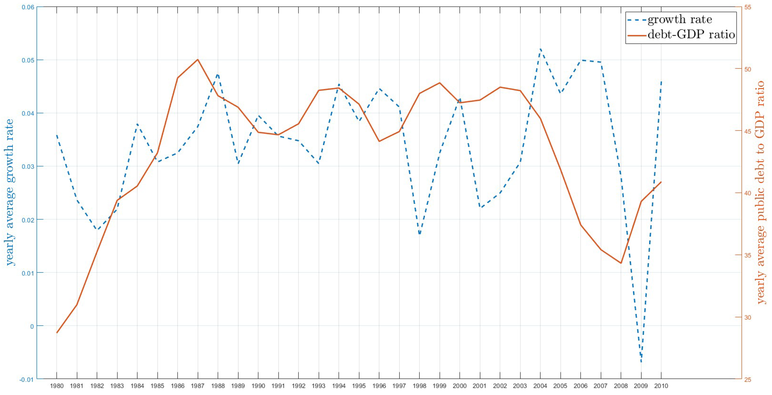
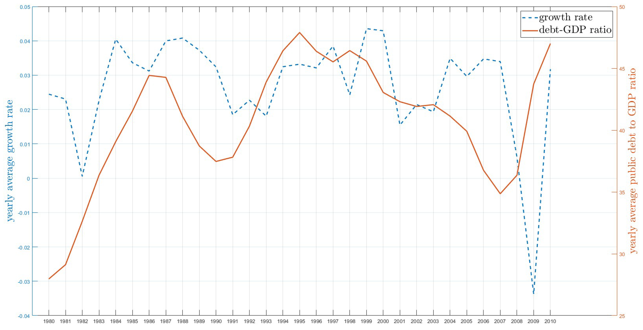
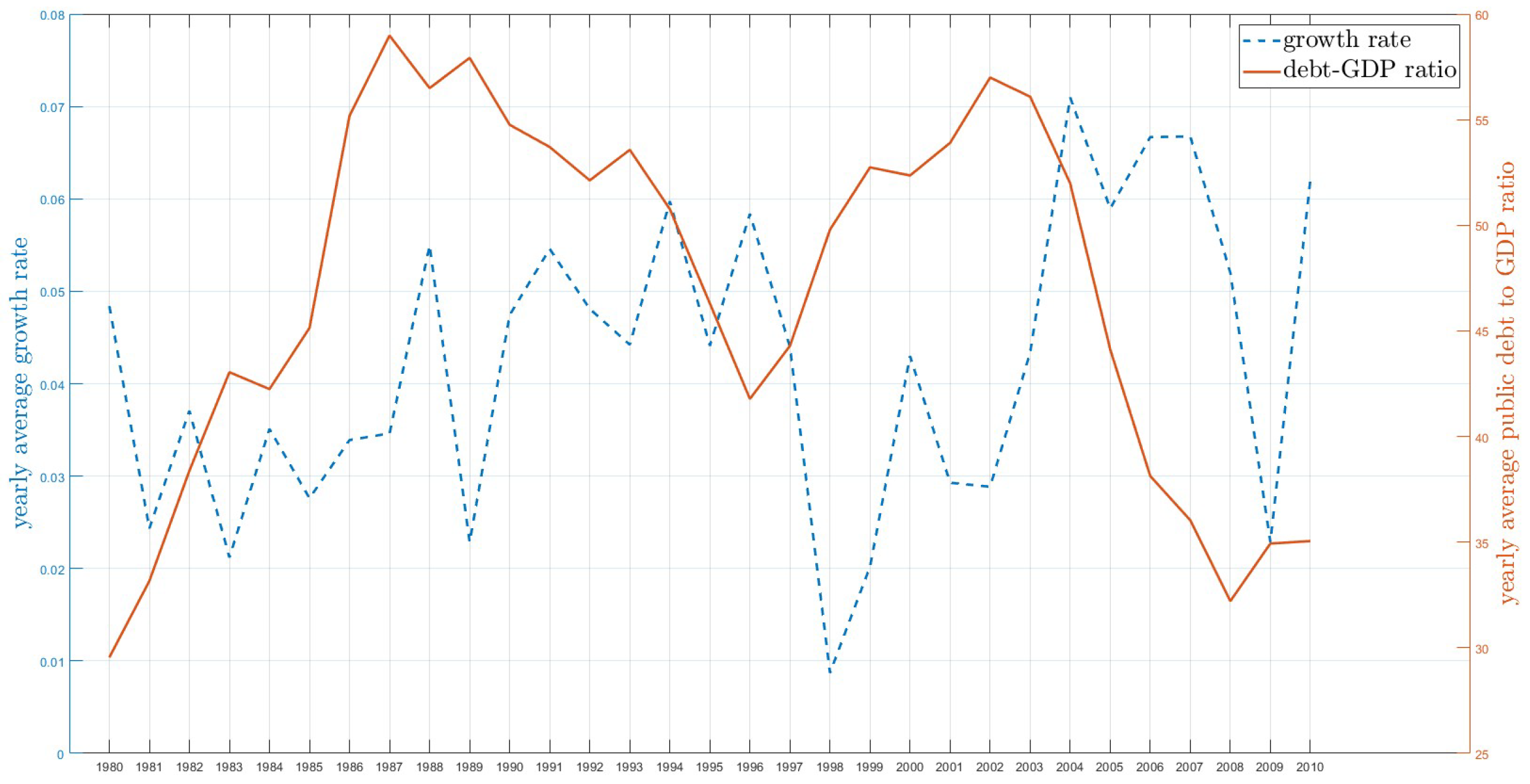
5.1. Data
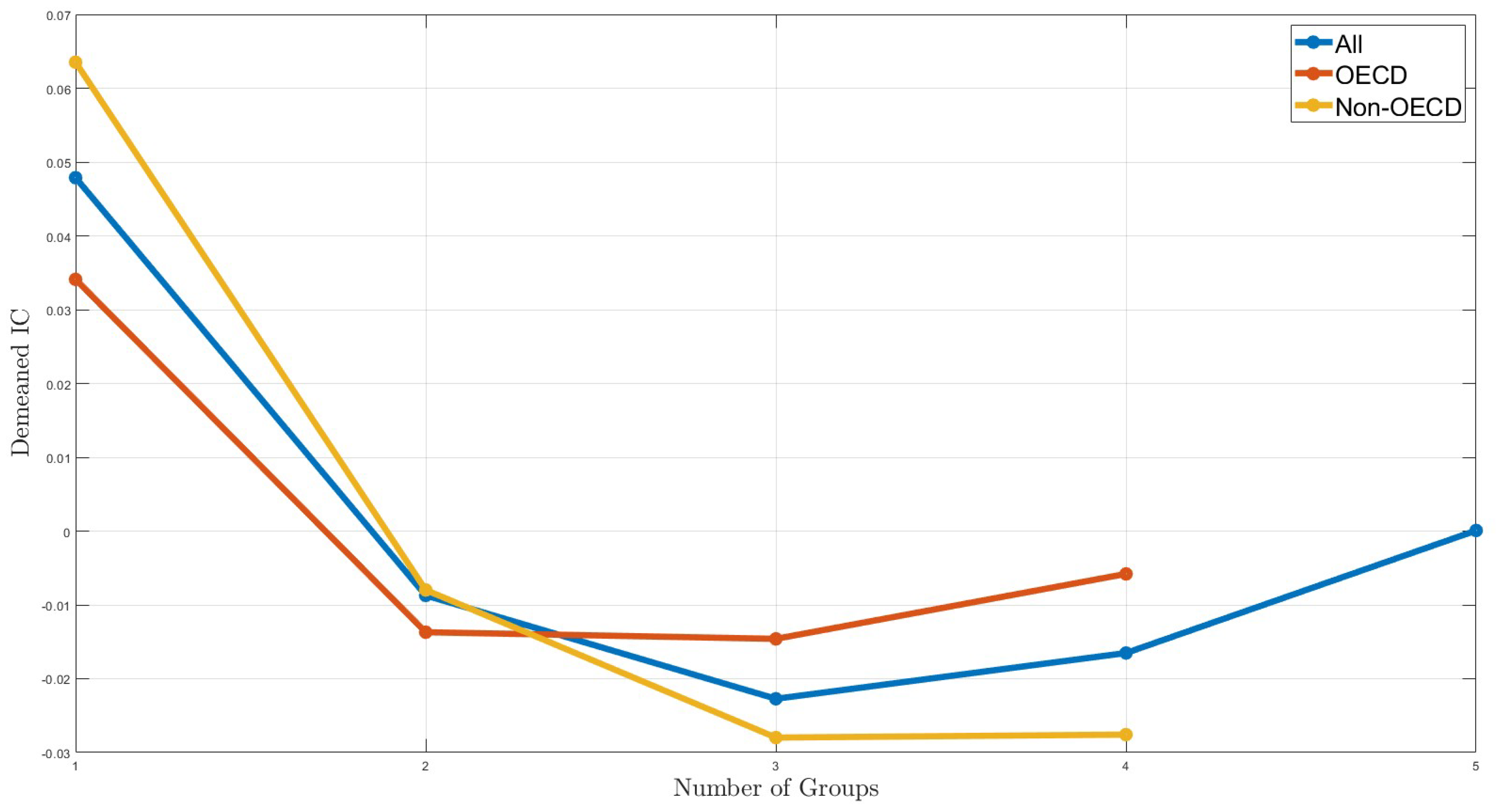
5.2. Identifying the Number of Groups
5.3. Estimation Results
6. Conclusions
Author Contributions
Funding
Data Availability Statement
Conflicts of Interest
Appendix A. Lemmas
Appendix B. Theorem
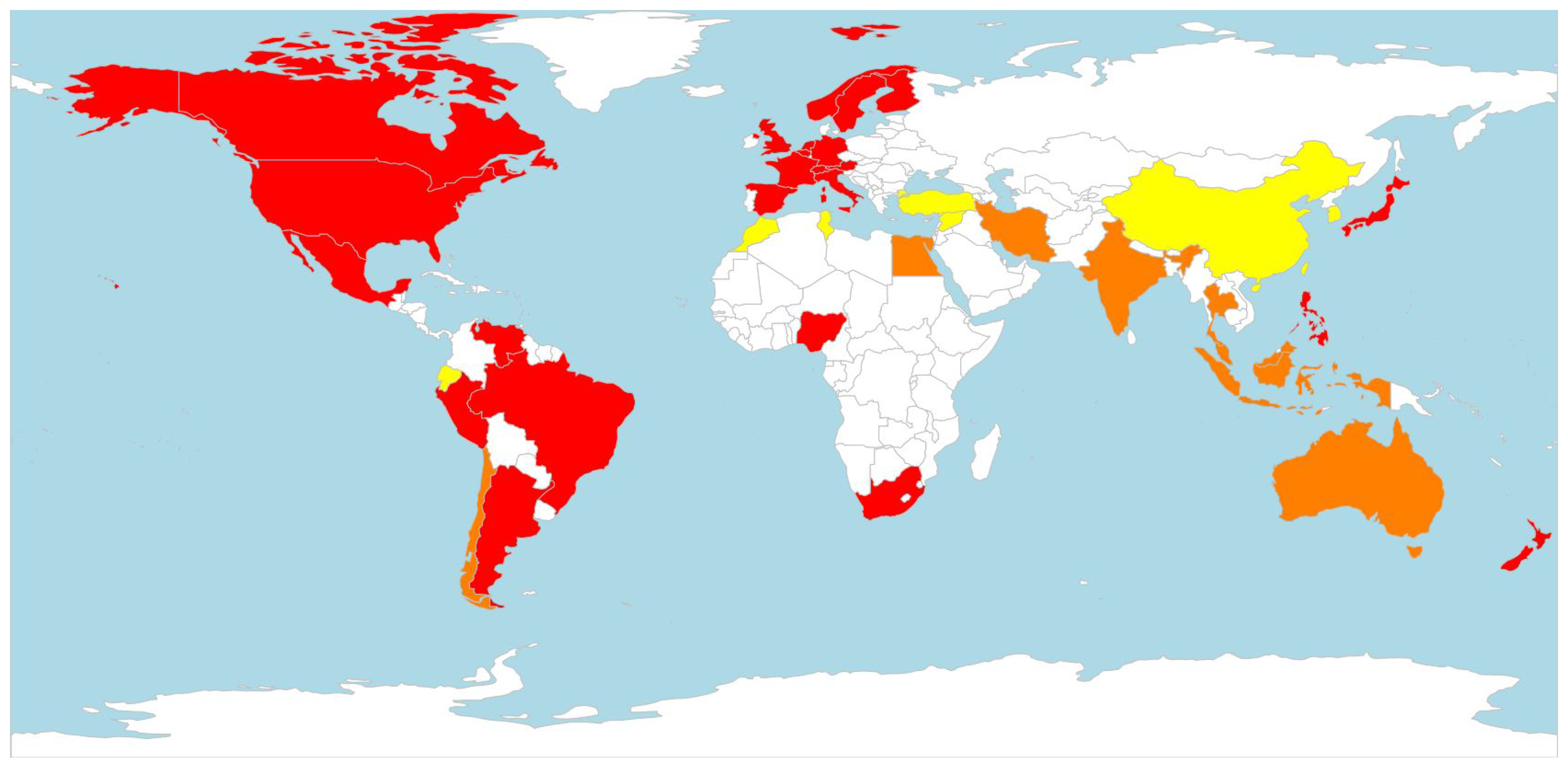
Appendix C. List of Countries

| Country | OECD | Country | OECD |
|---|---|---|---|
| Argentina | Mexico | √ | |
| Australia | √ | Morocco | |
| Austria | √ | Netherlands | √ |
| Belgium | √ | New Zealand | √ |
| Brazil | Nigeria | ||
| Canada | √ | Norway | √ |
| Chile | √ | Peru | |
| China | Philippines | ||
| Ecuador | Singapore | ||
| Egypt, Arab Rep. | South Africa | ||
| Finland | √ | Spain | √ |
| France | √ | Sweden | √ |
| Germany | √ | Switzerland | √ |
| India | Syria | ||
| Indonesia | Thailand | ||
| Iran, Islamic Rep. | Tunisia | ||
| Italy | √ | Turkey | √ |
| Japan | √ | United Kingdom | √ |
| Korea, Rep. | √ | United States | √ |
| Malaysia | Venezuela |
| 1 | Zhang et al. (2023) study the endogenous kink regression model by applying a nonparametric control function approach. Their method can be extended to our latent structure model. We leave this for future study. |
| 2 | Including can be attractive for other applications. However, in our empirical study, we only include the constant term, assuming |
| 3 | We exclude the panel nonstationary regressors. Chen and Stengos (2022) study a threshold model with hybrid stochastic local unit root regressors. Their study offers a potential extension to the panel kink regression model. We leave this for future study. |
| 4 | |
| 5 | In the empirical application, as suggested by Miao et al. (2020), we use . |
| 6 | The IC values for various groupings are as follows: For the full sample of all countries, the IC values are −6.6269, −6.6835, −6.6975, −6.6913, −6.6747 for , respectively. For OECD countries, the IC values are −7.1278, −7.1756, −7.1765, and −7.1677, corresponding to . For non-OECD countries, the values are −6.3126, −6.3841, −6.4041, and −6.4037 for , respectively. |
References
- Afonso, António, and João Tovar Jalles. 2013. Growth and productivity: The role of government debt. International Review of Economics & Finance 25: 384–407. [Google Scholar]
- Barro, Robert J. 1974. Are government bonds net wealth? Journal of Political Economy 82: 1095–117. [Google Scholar] [CrossRef]
- Baum, Anja, Cristina Checherita-Westphal, and Philipp Rother. 2013. Debt and growth: New evidence for the euro area. Journal of International Money and Finance 32: 809–21. [Google Scholar] [CrossRef]
- Blanchard, Olivier J. 1985. Debt, deficits, and finite horizons. Journal of Political Economy 93: 223–47. [Google Scholar] [CrossRef]
- Bonhomme, Stéphane, Thibaut Lamadon, and Elena Manresa. 2022. Discretizing unobserved heterogeneity. Econometrica 90: 625–43. [Google Scholar] [CrossRef]
- Bonhomme, Stéphane, and Elena Manresa. 2015. Grouped patterns of heterogeneity in panel data. Econometrica 83: 1147–84. [Google Scholar] [CrossRef]
- Caner, Mehmet, Thomas Grennes, and Fritzi Koehler-Geib. 2010. Finding the tipping point: When sovereign debt turns bad. Sovereign Debt and the Financial Crisis 63–75. Available online: https://papers.ssrn.com/sol3/papers.cfm?abstract_id=1612407 (accessed on 15 October 2023).
- Cecchetti, Stephen G., Madhusudan S. Mohanty, and Zampolli Fabrizio. 2011. The Real Effects of Debt. Bank for International Settlements Working Papers No 352. Basel: Bank for International Settlements. [Google Scholar]
- Chan, Kung-Sik. 1993. Consistency and limiting distribution of the least squares estimator of a threshold autoregressive model. The Annals of Statistics 21: 520–33. [Google Scholar] [CrossRef]
- Chan, Kung-Sig, and Ruey S. Tsay. 1998. Limiting properties of the least squares estimator of a continuous threshold autoregressive model. Biometrika 85: 413–26. [Google Scholar] [CrossRef]
- Chen, Chaoyi, and Thanasis Stengos. 2022. Estimation and inference for the threshold model with hybrid stochastic local unit root regressors. Journal of Risk and Financial Management 15: 242. [Google Scholar] [CrossRef]
- Chen, Chaoyi, Thanasis Stengos, and Yiguo Sun. 2023. Endogeneity in semiparametric threshold regression models with two threshold variables. Econometric Reviews 42: 758–79. [Google Scholar] [CrossRef]
- Chudik, Alexander, Kamiar Mohaddes, M. Hashem Pesaran, and Mehdi Raissi. 2017. Is there a debt-threshold effect on output growth? Review of Economics and Statistics 99: 135–50. [Google Scholar] [CrossRef]
- Eberhardt, Markus, and Andrea F. Presbitero. 2015. Public debt and growth: Heterogeneity and non-linearity. Journal of International Economics 97: 45–58. [Google Scholar] [CrossRef]
- Elmendorf, Douglas W., and N. Gregory Mankiw. 1999. Chapter 25 government debt. Handbook of Macroeconomics 1: 1615–69. [Google Scholar]
- Frankel, Jeffrey A., and David Romer. 1999. Does trade cause growth? American Economic Review 89: 379–99. [Google Scholar] [CrossRef]
- Gómez-Puig, Marta, Simón Sosvilla-Rivero, and Inmaculada Martínez-Zarzoso. 2022. On the heterogeneous link between public debt and economic growth. Journal of International Financial Markets, Institutions and Money 77: 101528. [Google Scholar] [CrossRef]
- Hansen, Bruce E. 2000. Sample splitting and threshold estimation. Econometrica 68: 575–603. [Google Scholar] [CrossRef]
- Hansen, Bruce E. 2017. Regression kink with an unknown threshold. Journal of Business & Economic Statistics 35: 228–40. [Google Scholar]
- Hidalgo, Javier, Jungyoon Lee, and Myung Hwan Seo. 2019. Robust inference for threshold regression models. Journal of Econometrics 210: 291–309. [Google Scholar] [CrossRef]
- Kourtellos, Andros, Thanasis Stengos, and Chih Ming Tan. 2013. The effect of public debt on growth in multiple regimes. Journal of Macroeconomics 38: 35–43. [Google Scholar] [CrossRef]
- Miao, Ke, Liangjun Su, and Wendun Wang. 2020. Panel threshold regressions with latent group structures. Journal of Econometrics 214: 451–81. [Google Scholar] [CrossRef]
- Panizza, Ugo, and Andrea F. Presbitero. 2013. Public debt and economic growth in advanced economies: A survey. Swiss Journal of Economics and Statistics 149: 175–204. [Google Scholar] [CrossRef]
- Reinhart, Carmen M., and Kenneth S. Rogoff. 2010. Growth in a time of debt. American Economic Review 100: 573–78. [Google Scholar] [CrossRef]
- Su, Liangjun, and Qihui Chen. 2013. Testing homogeneity in panel data models with interactive fixed effects. Econometric Theory 29: 1079–135. [Google Scholar] [CrossRef]
- Su, Liangjun, Zhentao Shi, and Peter C. Phillips. 2016. Identifying latent structures in panel data. Econometrica 84: 2215–64. [Google Scholar] [CrossRef]
- Zhang, Jianhan, Chaoyi Chen, Yiguo Sun, and Thanasis Stengos. 2023. Endogenous kink threshold regression. SSRN Electronic Journal. Available online: https://ssrn.com/abstract=4742634 (accessed on 1 February 2024).


| Group 1 | Group 2 | Group 3 | ||||||||
|---|---|---|---|---|---|---|---|---|---|---|
| MSE | ||||||||||
| N = 50 | T = 30 | 0.014 | 0.030 | 0.209 | 0.007 | 0.017 | 0.126 | 0.458 | 0.035 | 0.336 |
| N = 100 | T = 30 | 0.010 | 0.007 | 0.107 | 0.005 | 0.003 | 0.065 | 0.007 | 0.010 | 0.118 |
| N = 50 | T = 60 | 0.043 | 0.141 | 0.173 | 0.004 | 0.003 | 0.051 | 0.007 | 0.186 | 0.170 |
| N = 100 | T = 60 | 0.002 | 0.002 | 0.027 | 0.002 | 0.001 | 0.030 | 0.003 | 0.003 | 0.033 |
| BIAS | ||||||||||
| N = 50 | T = 30 | −0.019 | 0.049 | 0.030 | −0.014 | 0.030 | 0.010 | −0.069 | 0.054 | 0.064 |
| N = 100 | T = 30 | −0.021 | −0.011 | −0.037 | −0.006 | 0.002 | −0.003 | −0.010 | 0.015 | 0.019 |
| N = 50 | T = 60 | −0.030 | 0.053 | 0.012 | −0.012 | 0.001 | −0.049 | −0.010 | 0.069 | 0.018 |
| N = 100 | T = 60 | 0.001 | 0.009 | 0.024 | 0.001 | 0.005 | 0.009 | −0.013 | 0.004 | −0.026 |
| STD | ||||||||||
| N = 50 | T = 30 | 0.118 | 0.166 | 0.457 | 0.085 | 0.127 | 0.355 | 0.673 | 0.180 | 0.576 |
| N = 100 | T = 30 | 0.100 | 0.081 | 0.325 | 0.067 | 0.057 | 0.254 | 0.081 | 0.098 | 0.343 |
| N = 50 | T = 60 | 0.205 | 0.371 | 0.416 | 0.066 | 0.053 | 0.219 | 0.082 | 0.426 | 0.412 |
| N = 100 | T = 60 | 0.042 | 0.042 | 0.163 | 0.040 | 0.037 | 0.173 | 0.051 | 0.050 | 0.179 |
| Group 1 | Group 2 | Group 3 | ||||||||
|---|---|---|---|---|---|---|---|---|---|---|
| MSE | ||||||||||
| N = 50 | T = 30 | 0.139 | 0.731 | 0.391 | 0.024 | 0.401 | 0.288 | 0.011 | 0.043 | 0.255 |
| N = 100 | T = 30 | 0.016 | 0.003 | 0.099 | 0.003 | 0.003 | 0.035 | 0.006 | 0.033 | 0.144 |
| N = 50 | T = 60 | 0.028 | 0.010 | 0.135 | 0.005 | 0.004 | 0.074 | 0.036 | 0.034 | 0.173 |
| N = 100 | T = 60 | 0.007 | 0.001 | 0.055 | 0.001 | 0.001 | 0.020 | 0.001 | 0.010 | 0.072 |
| BIAS | ||||||||||
| N = 50 | T = 30 | −0.100 | 0.112 | 0.008 | −0.016 | 0.122 | 0.065 | −0.028 | 0.051 | −0.044 |
| N = 100 | T = 30 | −0.025 | 0.017 | 0.021 | −0.003 | 0.006 | 0.018 | −0.018 | 0.030 | −0.005 |
| N = 50 | T = 60 | −0.036 | 0.008 | −0.013 | −0.018 | 0.005 | −0.046 | −0.019 | 0.031 | 0.008 |
| N = 100 | T = 60 | −0.010 | 0.009 | 0.020 | 0.001 | 0.004 | 0.002 | −0.004 | 0.025 | −0.005 |
| STD | ||||||||||
| N = 50 | T = 30 | 0.164 | 0.098 | 0.368 | 0.069 | 0.062 | 0.268 | 0.188 | 0.182 | 0.416 |
| N = 100 | T = 30 | 0.085 | 0.035 | 0.233 | 0.036 | 0.036 | 0.140 | 0.033 | 0.097 | 0.268 |
| N = 50 | T = 60 | 0.359 | 0.847 | 0.625 | 0.153 | 0.622 | 0.533 | 0.102 | 0.200 | 0.504 |
| N = 100 | T = 60 | 0.124 | 0.056 | 0.314 | 0.059 | 0.052 | 0.186 | 0.076 | 0.179 | 0.380 |
| N = 50 | N = 100 | N = 50 | N = 100 | |
| T = 30 | 0.0036 | 0.0021 | 0.0114 | 0.0088 |
| T = 60 | 0 | 0 | 0.004 | 0.002 |
| Group 1 | Group 2 | Group 3 | ||||||||||
|---|---|---|---|---|---|---|---|---|---|---|---|---|
| MSE | 0.001 | 0.009 | 0.023 | 0.004 | 0.000 | 0.011 | 0.017 | 0.003 | 0.000 | 0.016 | 0.027 | 0.002 |
| 0.001 | 0.005 | 0.011 | 0.002 | 0.000 | 0.006 | 0.013 | 0.002 | 0.000 | 0.014 | 0.015 | 0.002 | |
| 0.000 | 0.002 | 0.006 | 0.002 | 0.000 | 0.003 | 0.007 | 0.001 | 0.000 | 0.004 | 0.007 | 0.001 | |
| 0.000 | 0.002 | 0.004 | 0.001 | 0.000 | 0.002 | 0.004 | 0.000 | 0.000 | 0.003 | 0.005 | 0.001 | |
| BIAS | 0.006 | 0.018 | −0.068 | 0.016 | 0.005 | −0.029 | −0.037 | 0.036 | −0.001 | −0.095 | 0.007 | 0.040 |
| 0.009 | 0.007 | −0.060 | 0.020 | 0.006 | −0.036 | −0.062 | 0.031 | 0.001 | −0.096 | −0.015 | 0.041 | |
| 0.001 | −0.011 | −0.021 | 0.015 | 0.002 | −0.022 | −0.031 | 0.016 | 0.001 | −0.047 | −0.021 | 0.019 | |
| 0.001 | −0.015 | −0.026 | 0.013 | 0.002 | −0.019 | −0.036 | 0.013 | 0.000 | −0.040 | −0.034 | 0.017 | |
| STD | 0.031 | 0.094 | 0.134 | 0.058 | 0.017 | 0.099 | 0.125 | 0.038 | 0.015 | 0.081 | 0.163 | 0.029 |
| 0.021 | 0.072 | 0.085 | 0.044 | 0.012 | 0.068 | 0.094 | 0.026 | 0.010 | 0.068 | 0.123 | 0.024 | |
| 0.020 | 0.048 | 0.077 | 0.039 | 0.011 | 0.047 | 0.078 | 0.024 | 0.009 | 0.047 | 0.079 | 0.018 | |
| 0.013 | 0.036 | 0.054 | 0.028 | 0.008 | 0.036 | 0.048 | 0.017 | 0.007 | 0.042 | 0.064 | 0.015 | |
| Group 1 | Group 2 | Group 3 | ||||||||||
|---|---|---|---|---|---|---|---|---|---|---|---|---|
| MSE | 0.001 | 0.016 | 0.011 | 0.005 | 0.000 | 0.007 | 0.018 | 0.002 | 0.001 | 0.012 | 0.053 | 0.006 |
| 0.001 | 0.006 | 0.005 | 0.003 | 0.000 | 0.006 | 0.010 | 0.002 | 0.001 | 0.007 | 0.045 | 0.004 | |
| 0.000 | 0.006 | 0.004 | 0.002 | 0.000 | 0.003 | 0.007 | 0.001 | 0.000 | 0.003 | 0.026 | 0.002 | |
| 0.000 | 0.002 | 0.002 | 0.001 | 0.000 | 0.002 | 0.004 | 0.001 | 0.000 | 0.002 | 0.012 | 0.001 | |
| BIAS | 0.017 | −0.036 | −0.046 | 0.030 | 0.003 | −0.050 | −0.053 | 0.032 | −0.022 | −0.080 | −0.089 | 0.068 |
| 0.017 | −0.015 | −0.045 | 0.025 | 0.001 | −0.059 | −0.042 | 0.035 | −0.020 | −0.067 | −0.105 | 0.061 | |
| 0.011 | −0.015 | −0.021 | 0.015 | 0.001 | −0.027 | −0.037 | 0.015 | −0.011 | −0.041 | −0.046 | 0.034 | |
| 0.010 | −0.004 | −0.025 | 0.011 | 0.001 | −0.025 | −0.036 | 0.015 | −0.010 | −0.035 | −0.048 | 0.029 | |
| STD | 0.028 | 0.123 | 0.095 | 0.061 | 0.016 | 0.069 | 0.125 | 0.035 | 0.015 | 0.071 | 0.213 | 0.036 |
| 0.018 | 0.075 | 0.059 | 0.044 | 0.011 | 0.046 | 0.091 | 0.025 | 0.011 | 0.050 | 0.184 | 0.025 | |
| 0.017 | 0.076 | 0.062 | 0.042 | 0.011 | 0.048 | 0.078 | 0.023 | 0.009 | 0.040 | 0.154 | 0.020 | |
| 0.014 | 0.046 | 0.038 | 0.028 | 0.007 | 0.035 | 0.052 | 0.016 | 0.007 | 0.033 | 0.097 | 0.016 | |
| N = 50 | N = 100 | N = 50 | N = 100 | |
| T = 30 | 0.0038 | 0.005 | 0.057 | 0.0539 |
| T = 60 | 0 | 0 | 0.005 | 0.0064 |
| Latent Group | ✓ | |||
|---|---|---|---|---|
| G1 | G2 | G3 | ||
| 3.7020 | 3.7773 | 3.7906 | 4.0630 | |
| 0.0190 *** | 0.0391 *** | 0.0402 *** | 0.0190 *** | |
| (0.0023) | (0.0055) | (0.0053) | (0.0026) | |
| 0.3366 *** | −0.0842 | 0.3035 *** | 0.2975 *** | |
| (0.0388) | (0.0775) | (0.0626) | (0.0579) | |
| −0.0057 ** | −0.0315 *** | 0.0147 *** | 0.0084 *** | |
| (0.0028) | (0.0044) | (0.0044) | (0.0029) | |
| 0.0076 ** | 0.0022 | 0.0061 | 0.0032 | |
| (0.0037) | (0.0083) | (0.0077) | (0.0066) | |
| Country | 40 | 7 | 9 | 24 |
| Latent Group | ✓ | |||
|---|---|---|---|---|
| G1 | G2 | G3 | ||
| 3.6366 | 2.8289 | 4.4960 | 3.9997 | |
| 0.0205 *** | 0.0304 *** | 0.0169 ** | 0.0192 *** | |
| (0.0026) | (0.0068) | (0.0070) | (0.0022) | |
| 0.2864 *** | 0.0455 | 0.0768 | 0.2855 *** | |
| (0.0539) | (0.1289) | (0.1047) | (0.0600) | |
| 0.0005 | 0.0036 | −0.0239 *** | 0.0069 *** | |
| (0.0030) | (0.0074) | (0.0075) | (0.0026) | |
| −0.0042 | 0.0217 *** | 0.0473 | −0.0102 * | |
| (0.0042) | (0.0082) | (0.0389) | (0.0059) | |
| Country | 21 | 3 | 2 | 16 |
| Latent Group | ✓ | |||
|---|---|---|---|---|
| G1 | G2 | G3 | ||
| 3.7685 | 3.8292 | 4.3691 | 4.1174 | |
| 0.0224 *** | 0.0381 *** | 0.0314 *** | 0.0244 *** | |
| (0.0038) | (0.0062) | (0.0070) | (0.0058) | |
| 0.3078 *** | 0.3512 *** | −0.1717 | 0.3224 *** | |
| (0.0536) | (0.0760) | (0.1108) | (0.0810) | |
| −0.0111 ** | 0.0166 * | −0.0326 *** | 0.0256 *** | |
| (0.0044) | (0.0084) | (0.0046) | (0.0080) | |
| 0.0142 ** | −0.0049 | 0.0285 | 0.0530 *** | |
| (0.0056) | (0.0072) | (0.0173) | (0.0188) | |
| Country | 19 | 8 | 4 | 7 |
Disclaimer/Publisher’s Note: The statements, opinions and data contained in all publications are solely those of the individual author(s) and contributor(s) and not of MDPI and/or the editor(s). MDPI and/or the editor(s) disclaim responsibility for any injury to people or property resulting from any ideas, methods, instructions or products referred to in the content. |
© 2024 by the authors. Licensee MDPI, Basel, Switzerland. This article is an open access article distributed under the terms and conditions of the Creative Commons Attribution (CC BY) license (https://creativecommons.org/licenses/by/4.0/).
Share and Cite
Chen, C.; Stengos, T.; Zhang, J. Public Debt and Economic Growth: A Panel Kink Regression Latent Group Structures Approach. Econometrics 2024, 12, 7. https://doi.org/10.3390/econometrics12010007
Chen C, Stengos T, Zhang J. Public Debt and Economic Growth: A Panel Kink Regression Latent Group Structures Approach. Econometrics. 2024; 12(1):7. https://doi.org/10.3390/econometrics12010007
Chicago/Turabian StyleChen, Chaoyi, Thanasis Stengos, and Jianhan Zhang. 2024. "Public Debt and Economic Growth: A Panel Kink Regression Latent Group Structures Approach" Econometrics 12, no. 1: 7. https://doi.org/10.3390/econometrics12010007
APA StyleChen, C., Stengos, T., & Zhang, J. (2024). Public Debt and Economic Growth: A Panel Kink Regression Latent Group Structures Approach. Econometrics, 12(1), 7. https://doi.org/10.3390/econometrics12010007