The Gini and Mean Log Deviation Indices of Multivariate Inequality of Opportunity

Abstract

The most common approach to measuring inequality of opportunity in income is to apply the Gini inequality index or the Mean Log Deviation (MLD) index to a smoothed distribution (i.e., a distribution of type mean incomes). We show how this approach can be naturally extended to include life outcomes other than income (e.g., health, education). We propose two measures: the Gini and MLD indices of multivariate inequality of opportunity. We show that they can be decomposed into the contribution of each outcome and the dependence of the outcomes. Using these measures, we calculate inequality of opportunity in health and income across European countries.

1. Introduction

In recent years, the concept of Equality of Opportunity (EOP for short) has gained significant prominence in public policy discussions. It lies at the core of the policy-making of many countries and organizations; for example, it is part of the European Union’s growth strategy and the United Kingdom’s “levelling up” of citizens and regions. Broadly speaking, EOP argues that differences in life outcomes should be the result of individual effort and choice, rather than factors beyond the individual’s control, known as circumstances. It is a widely respected theory of fairness developed in political philosophy (e.g., Rawls 1971; Dworkin 1981; Arneson 1989; Cohen 1989; Roemer 1993, 1998) with applied quantitative models developed in the economics literature (Roemer 1993, 1998; Fleurbaey 1995, 2008; Van de Gaer 1993). Equality of opportunity has become a central tenet in political discourse, leading to a surge in academic research on the topic (see Ferreira and Peragine 2016; Ramos and Van de Gaer 2016; Roemer and Trannoy 2015 for recent surveys). In contrast to pure inequality, which measures inequality in today’s incomes, inequality of opportunity (IOP) focuses on the sources of today’s inequality located in the past. It links today’s income inequality to differences in past conditions, such as parental education or household income when the respondent was a child. Such early differences account for unequal starts in life and—as the literature shows—have an impact on future life outcomes. Given the IOP framework, pure income inequality can thus be thought of as consisting of two types of inequality, namely inequality due to past conditions that are beyond individual control (inequality of opportunity) and a residual component reflecting inequality due to individual effort.

EOP is becoming increasingly important as recent research shows that its lack can be detrimental to economic growth (Marrero and Rodríguez 2013; Ferreira et al. 2018; Aiyar and Ebeke 2020). In particular, several research papers (Marrero and Rodríguez 2013; Brunori et al. 2023; Marrero et al. 2016; Hsieh et al. 2019) showed that inequality of opportunity is negatively related to economic growth. There are two main channels of transmission: first, unequal access to resources leads to lower human capital accumulation among poorer individuals; second, inequality of opportunity creates a perception that it is not worth to put in effort, because outcomes depend on circumstances beyond the individual’s control, which may further reduce investment in human capital. At the same time, there is little consensus in the literature on the precise relationship between pure income inequality and growth. Recently, Aiyar and Ebeke (2020) show that this may be due to the lack of consideration of IOP in empirical analyses. They show that the relationship between inequality and economic growth is conditioned on inequality of opportunity. In societies with greater inequality of opportunity, income inequality exerts a greater drag on future growth. The greater the inequality of opportunity, the more negative the impact of inequality on economic growth.1 EOP becomes an attractive policy objective not only for reasons of social justice, but also for purely economic reasons.

Recent developments in the inequality of opportunity literature relate to the development of advanced computational methods (Brunori et al. 2023), the measurement of long-term inequality of opportunity (Aaberge et al. 2011; Bussolo et al. 2023), and the measurement of inequality of opportunity jointly across multiple life outcomes (Kapera et al. 2023). This paper relates to the latter strand of ongoing research. The traditional focus has been on income and our description so far also refers to income inequality and income inequality of opportunity. However, the understanding of well-being has expanded to include multidimensional factors beyond income (Stiglitz et al. 2010). Inequality measurement theory has followed suit, and multivariate measures of inequality have emerged (see Aaberge and Brandolini 2015 for the latest survey). However, this is not the case for inequality of opportunity. Despite the recognition of the multivariate nature of well-being and the fact that a multivariate extension of inequality of opportunity theory has been called for (Bourguignon et al. 2007), existing methods for measuring inequality of opportunity have long remained underdeveloped. As a result, various researchers have analysed IOP in different outcomes (e.g., Peragine and Serlenga 2008; de Barros et al. 2009; Ferreira and Gignoux 2010, 2011), but treated them as separate, thus losing information on their dependence, which is not neutral for multivariate measurement. Depending on whether the outcomes are treated as substitutes or complements, their higher dependence is considered to increase (or decrease) multivariate inequality beyond the effects of the respective dimensions (Atkinson and Bourguignon 1982). The inclusion of this information in this paper is ensured by taking a joint welfare function that is sensitive to dimension dependence. Furthermore, treating outcomes jointly allows for arrival at a unified conclusion in particular when univariate conclusions diverge.

Research in the multivariate direction has only recently begun with Kapera et al. (2023), who developed a theory of multivariate inequality of opportunity. They did so in an axiomatic framework in which ethical postulates of EOP are developed in the form of properties of social welfare functions and linked to multivariate measures of IOP. These measures are thus normative in the sense that a reduction in IOP leads to an increase in welfare, following the classical approach of Atkinson (1970) to the construction of inequality indices. They applied the axiomatic method to the area of inequality of opportunity, which has only recently been performed for a single outcome (income) (Bosmans and Öztürk 2021). Thus, they introduced a fully developed theory of multivariate IOP. As the most practical consequence, they characterized (i.e., derived from axioms) a relative multivariate IOP measure which is a standard multidimensional inequality index (Tsui 1995) applied to the multidimensional IOP framework. The measure has the advantage of being easily interpreted as reflecting two components: inequality between types (a type being a set of individuals with the same circumstances, e.g., low parental background) and inequality within types. It is sensitive to both the spread of the respective outcomes and their dependence, so it is truly a multivariate measure. From a purely theoretical point of view, our goal in this paper is much less ambitious, as we do not develop measures axiomatically. On the other hand, our measures have a higher application potential, since the Gini index and the Mean Logarithmic Deviation are much more used in applied research than the Tsui index, especially in the area of income inequality of opportunity. In fact, we are not aware of any application of the Tsui index to income IOP. Therefore, we propose measures that are more familiar to researchers working in the area of equality of opportunity. Furthermore, the measure in Kapera et al. (2023) has an additional vector of exogenous weights that must be chosen by the researcher. Our measures do not have this complication.

Let us now describe in more detail what we achieve in the paper. The most widely used approach to measuring inequality of opportunity for a single outcome (typically income) is based on two principles: ex ante compensation (which advocates equalizing inequalities among individuals with the same circumstances—types) and the utilitarian principle of reward (which deems any inequality arising within types, for example, due to differential individual effort, irrelevant). In practice, utilitarian reward is fulfilled by smoothing the distribution within a type by assigning to each individual in a type a type’s mean income. Then, consistently with ex ante compensation, an inequality index is applied to such smoothed distribution. The index then measures inequality between types. Indeed, the most popular approach to the measurement of IOP is between-group inequality, with groups defined by circumstances. Typically, the Gini index or the Mean Log Deviation are used as inequality indices. This approach has been used in numerous empirical papers (for a survey, please see, e.g., Ferreira and Peragine 2016 or Ramos and Van de Gaer 2016).

We offer a simple extension of this approach to multiple outcomes, i.e., taking into account, in addition to income, other dimensions of well-being such as health and education. The index then measures the extent to which these outcomes are jointly determined by past circumstances. Therefore, instead of looking only at income, we offer to look at welfare, in line with the welfarist tradition in the measurement of inequality (Dardanoni 1992; Maasoumi 1986). Welfare is measured by the Cobb–Douglas utility function applied to the type mean distribution which, as mentioned, is a distribution such that each individual in a type is assigned the mean value in that type of each attribute. This reflects the use of type mean incomes in the standard case and ensures consistency with the utilitarian reward. The Cobb–Douglas utility is sensitive to both inequality in respective outcomes and to their dependence, which reflects the multidimensional nature of our measure. The index is normalised to the highest welfare achieved for the perfectly equal distribution, i.e., the distribution of population means. We rely on Sen’s (Sen 1973; Dutta 2002) formulation of the Gini index, in which linear weights are assigned to types according to the ranking of type welfare, with the highest weight assigned the type with the lowest welfare. The construction of the MLD is similar, namely type mean income is replaced by type mean welfare. The use of such defined welfare has the advantage of the ability to decompose both indices into the contribution of the respective dimensions to the joint inequality and into the contribution of their dependence (in the case of the Gini)—the property known as attribute decomposability (Abul Naga and Geoffard 2006). It is useful in practical applications as it allows for better tracing the sources of the observed inequality. Policies to address inequalities can be very different depending on the dominant factor.

We apply our two measures to the European Union Statistics on Income and Living Conditions, which collects rich individual data across European countries. In the years 2005, 2011 and 2019, a special module was added to the main study, providing detailed information on family background. This made it possible to calculate inequality of opportunity. We use all three waves, as well as income and health as outcomes, and sex, age, parental education and occupation as circumstances. The average value of the Gini index is 20% of total inequality (i.e., “pure” inequality in the distribution of health and income) in 2005 and 25% in 2019. The MLD values are much lower2—8.6% in 2005 and 9.8% in 2019. Thus, by both measures, joint inequality of opportunity has increased on average in recent decades. Country rankings also change over the years. The most striking observation is that of three Scandinavian countries (Denmark, Norway and Sweden), which are either very or fairly unequal in terms of opportunity when more outcomes than incomes are taken into account. This is consistent with some other research (Heckman and Landersø 2002). The contribution of dependence to the Gini index is small—around 1.5%, which may be due to the smoothing of the distribution. The dominant factor is income (average contribution in 2019— 62%) and similarly for MLD (64%). The univariate health IOP and income IOP rankings of countries diverge a lot, which calls for a joint measure to arrive at a unified ranking.

All in all, we show how popular IOP measures used to measure income IOP can be naturally extended to measure IOP in multiple outcomes and illustrate their use with European data. In Section 2, we introduce notation, present the measures and also show their attribute decomposability (Lemmas 1 and 2). In Section 3, we present an empirical analysis and conclude.

2. The Measures

We have a society of N individuals and each individual is fully described by their outcomes, circumstances (factors beyond their control), and effort (factors within their control). Ex ante inequality concerns the situation before any effort is made, so the focus is on the opportunities available to individuals in a given set of circumstances. These are represented by the set of outcomes in a given circumstance group (called a type). The outcome distribution in type $X^h$ is thus the primitive of the model. It defines the opportunity set available to individuals in a type.

Formally, we divide society into n ordered types $1<\dots <n$. As mentioned, type h is a set of individuals with the same circumstances. We let $N_h$ be the number of people in type h; ${\sum }_{h=1}^n{N}_h=N$. Since we deal with the case of multivariate outcomes, $X^h$ comprises k outcomes for each individual. $M_{N_h\times k}$ is the set of all such matrices. We let $X\in M_{N\times k}$ represent outcome profile of the whole society and $M_{N\times k}$ be the set of all possible outcome profiles. $X^h$ and X give rise to two special distributions, namely a distribution in type h where every individual is assigned type’s h mean of each attribute, and a distribution where every individual is assigned a population mean of each attribute. We let $X_{\mu }\in M_{N\times k}$ be a matrix of type-means. It represents the case of perfect within-type equality, but not between-type equality. The latter is denoted $X^{\mu }\in M_{N\times k}$; it is a matrix of population means. Finally, $I:M_{N\times k}\to [0,1]$ is an index of inequality of opportunity. It is a continuous function taking the minimum value of 0 for the perfectly equal distribution (i.e., $I\left(X^{\mu }\right)=0$ and $I\left(X\right)\ge 0$).

There are two basic postulates of ex ante equality theory that are related to the widely used measures. First, there is the utilitarian principle of reward, which states that any inequality within a type is irrelevant. In other words, any form of inequality arising from differential effort is accepted. Second, there is the ex ante principle of compensation, which states that any inequality between types is undesirable. In practice, this is implemented by smoothing the within-type distribution by assigning each individual in a type the mean income of a type, and then calculating the inequality in such a smoothed vector of incomes. In effect, then, any within-type inequality is removed from the evaluation (consistent with utilitarian reward) and inequality is measured between types (consistent with the principle of compensation). As mentioned above, we follow this approach in a multidimensional setting. The difference is that instead of a vector of incomes, we have a vector of utilities, which are multivariate functions of k outcomes. Typically, smoothing takes the form of computing utility at the mean values of attributes. This produces type mean distribution $X_{\mu }$, and inequality measures are computed using this distribution. We focus on this approach, but we also comment on the second approach, which involves computing mean utility instead. Both forms are present in the literature on multidimensional inequality measures (see, for example, Aaberge and Brandolini 2015).

We measure welfare using the well-known Cobb–Douglas function as in, for example, Tsui (1995) multivariate inequality index, here applied to type mean distribution $X_{\mu }$, i.e., ${\prod }_{j=1}^k{\left({\left(X_{\mu }\right)}_j^h\right)}^{r_j}$. This utility function pays attention to both the spread in respective outcomes and to the outcome dependence. Parameters $r_j$ are dimensional weights; they correspond to the degree of inequality aversion. In particular, $r_j=1-{ϵ}_j$, where ${ϵ}_j$ is an inequality aversion parameter for dimension j (see, e.g., Atkinson 1970). As ${ϵ}_j$ increases, it becomes more efficient from a welfare point of view to reduce inequality at the bottom of the distribution than at the top, because with a higher degree of inequality aversion, a transfer at the bottom reduces inequality by more than the same transfer at the top. In his seminal paper, Atkinson (1970) arbitrarily set the income inequality aversion parameters to 1, 1.5 and 2. Since then, the empirical literature has attempted to estimate it from tax plans that are assumed to reflect societal preferences for redistribution in democratic societies (see, for example, Young 1990; Aristei and Perugini 2016).

Before proposing the first multivariate IOP measure, let us recall the univariate version of the Gini inequality index. The original formula for the Gini index is $G\left(y\right)=\frac{{\sum }_{i=1}^N{\sum }_{j=1}^N|y_i-y_j|}{2N^2\overline{y}}$, which provides its interpretation as one half of the relative mean difference. That is, the Gini measure computes the average income gap over all possible pairs of individuals in proportion to mean income $\overline{y}$.3 However, we use an equivalent formula for the Gini index according to Sen (1973). For a vector of decreasing individual incomes $y_i\ge y_{i+1}$ for all $i=1,\dots ,N$, we have

$$G\left(y\right)=1-\sum _{i=1}^N\frac{(2i-1)}{N^2}\frac{y_i}{\overline{y}},$$

(1)

where $\overline{y}$ denotes the mean income. Linear rank-based weights are inversely related to income values; the first individual $i=1$ that has the highest income obtains the lowest weight $(2\ast 1-1)=1$. Note that

$$N^2=2\frac{N(N+1)}{2}-N=2\left(\sum _{i=1}^{N}i\right)-N=\sum _{i=1}^N(2i-1).$$

Therefore, we can rewrite (1) as

$$G\left(y\right)=1-\sum _{i=1}^N\frac{(2i-1)}{{\sum }_{i=1}^N(2i-1)}\frac{y_i}{\overline{y}}.$$

(2)

Ina multivariate IOP measure, we replace i with h which denotes a type. Every individual in a type receives the same weight $(2h-1)$ (since their values are the same in a type) and there are $N_h$ individuals in a type; therefore, type weight is $N_h(2h-1)$. Furthermore, we replace income with welfare. As mentioned, this is measured by Cobb–Douglas function applied to type mean distribution $X_{\mu }$, i.e., ${\prod }_{j=1}^k{\left({\left(X_{\mu }\right)}_j^h\right)}^{r_j}$ and normalized by the welfare for perfectly equal distribution $X^{\mu }$ which is the distribution of population means for each attribute, similarly to mean income in (1). Types are ordered in descending order, i.e., $h=1$ denotes the type with the highest ${\prod }_{j=1}^k{\left(\frac{{\left(X_{\mu }\right)}_j^h}{{\left(X^{\mu }\right)}_j^h}\right)}^{r_j}$ and $h=n$ denotes the type with the lowest ${\prod }_{j=1}^k{\left(\frac{{\left(X_{\mu }\right)}_j^h}{{\left(X^{\mu }\right)}_j^h}\right)}^{r_j}$. In other words, a higher weight is assigned to a type with a lower value of the normalized utility of the type means. This ordering of types is thus based on outcomes consistent with the standard approach to ordering types. From the properties of the utility function (Aczél 1988), we know that for $r_j\in (0,1),{\sum }_{j=1}^k{r}_1\le 1$, it is concave and increasing, so $-{\prod }_{j=1}^k{\left({\left(X_{\mu }\right)}_j^h\right)}^{r_j}$ is convex.

A technical note: as you may have noticed, for the sake of brevity and clarity, we slightly abuse the notation by writing ${\left(X_{\mu }\right)}_j^h$ or ${\left(X^{\mu }\right)}_j$, whereas to be formally precise we should specify which specific row (individual) of these matrices we are taking. However, all rows in these matrices are the same, as they are matrices of type means and population means, respectively, so we omit additional subscripts. Finally, a multivariate analogue of (2) is

Definition 1. 

The Gini index of multivariate inequality of opportunity:

$$I_G\left(X\right)=1-\sum _{h=1}^n\frac{N_h(2h-1)}{{\sum }_{h=1}^n{N}_h(2h-1)}\prod _{j=1}^k{\left(\frac{{\left(X_{\mu }\right)}_j^h}{{\left(X^{\mu }\right)}_j}\right)}^{r_j},r_j\in (0,1),\sum _{j=1}^k{r}_1\le 1$$

(3)

Another index often used to measure income inequality of opportunity is the Mean Log Deviation. To recall, the univariate MLD index is as follows: for a vector of incomes $y_1,\dots ,y_N$, we have4

$$MLD\left(y\right)=\sum _{i=1}^N\frac{1}{N}ln\frac{\overline{y}}{y_i}.$$

(4)

Redefining this in a multivariate IOP framework, with individuals replaced by types of size $N_h$ and individual incomes with type mean values $X_{\mu }$, we obtain the following measure:

Definition 2. 

The Mean Log Deviation index of multivariate inequality of opportunity:

$$I_{MLD}\left(X\right)=\sum _{h=1}^n\frac{N_h}{{\sum }_{h=1}^n{N}_h}ln\prod _{j=1}^k{\left(\frac{{\left(X^{\mu }\right)}_j}{{\left(X_{\mu }\right)}_j^h}\right)}^{r_j},r_j>0$$

(5)

Parameters $r_j$ are again dimensional weights that appear in front of the logarithm because of the properties of the logarithm (which become clear in Lemma 2). Note the reverse order of $\frac{{\left(X^{\mu }\right)}_j^h}{{\left(X_{\mu }\right)}_j}$ compared to (3), which together with the logarithm ensures convexity.

In both measures, we use ${\prod }_{j=1}^k{\left({\left(X^{\mu }\right)}_j\right)}^{r_j}$ as the normalizing factor. This is the value of the highest welfare, which is the welfare for the perfectly equal distribution $X^{\mu }$. This is a natural normalization, e.g., Bourguignon (1999) writes: “maximising social welfare under the constraint of fixed total resources of attributes (...) requires giving each individual the average available quantity of attributes”. However, in the literature on multivariate inequality measurement, another normalization can be used, namely mean welfare (see, for example, Aaberge and Brandolini 2015). Then, type-mean welfare and mean welfare are as follows: ${\overline{u}}^h:=-\frac{1}{N_h}{\sum }_{i=1}^{N_h}{\prod }_{j=1}^k{\left(X_{ij}^h\right)}^{r_j}$ and $\overline{u}:=-\frac{1}{N}{\sum }_{i=1}^N{\prod }_{j=1}^k{\left(X_{ij}\right)}^{r_j}$, where $X_{ij}^h$ denotes the value of attribute j for individual i of type h and $X_{ij}$ the same without type membership. In other words, individual utilities are averaged within type and across the population. The Gini index then becomes $I_G\left(X\right)=1-\frac{1}{N^2}{\sum }_{h=1}^n{N}_h(2h-1)\frac{{\overline{u}}^h}{\overline{u}}$ and the MLD index is $I_{MLD}\left(X\right)={\sum }_{h=1}^n\frac{N_h}{{\sum }_{h=1}^n{N}_h(2h-1)}ln\frac{\overline{u}}{{\overline{u}}^h}$. We apply these measures to the data, too. For the Gini index, the results are almost unchanged, while for MLD they differ by around 10% percent.

Using the Cobb–Douglas utility function has the advantage of the possibility to decompose multivariate indices into the inequality of the respective outcomes and into the dependence of the outcomes. Abul Naga and Geoffard (2006) provide such a decomposition for multivariate equality measures. However, their aim and therefore their approach in this area is more ambitious because they develop a full theory by linking equality measures to welfare functions. We use their results to interpret the dependence measure. Furthermore, for equality measures, the decomposition can be exact, without the approximation which is needed for inequality measures (see, e.g., Zhong 2009).

For the sake of brevity, we present the case of $k=2$ outcomes, but this can be easily extended to any number of outcomes.

Lemma 1. 

The Gini multivariate IOP index (3) can be decomposed as

$$I_G\left(X\right)=I_G^1\left(X^1\right)+I_G^2\left(X^2\right)+(1-\kappa )+R,$$

(6)

where

$$\begin{array}{ccc}\hfill I_G^1\left(X^1\right)=1-\sum _{h=1}^n\frac{N_h(2h-1)}{{\sum }_{h=1}^n{N}_h(2h-1)}{\left(\frac{{\left(X_{\mu }\right)}_1^h}{{\left(X^{\mu }\right)}_1}\right)}^{r_1}& & \mathrm{I}\mathrm{O}\mathrm{P} (1\mathrm{s}\mathrm{t} \mathrm{o}\mathrm{u}\mathrm{t}\mathrm{c}\mathrm{o}\mathrm{m}\mathrm{e})\hfill \\ \hfill I_G^2\left(X^2\right)=1-\sum _{h=1}^n\frac{N_h(2h-1)}{{\sum }_{h=1}^n{N}_h(2h-1)}{\left(\frac{{\left(X_{\mu }\right)}_2^h}{{\left(X^{\mu }\right)}_2}\right)}^{r_2}& & \mathrm{I}\mathrm{O}\mathrm{P} (2\mathrm{n}\mathrm{d} \mathrm{o}\mathrm{u}\mathrm{t}\mathrm{c}\mathrm{o}\mathrm{m}\mathrm{e})\hfill \\ \hfill \kappa \left(X\right)=1-\frac{\left[{\sum }_{h=1}^n{N}_h(2h-1)\right]{\sum }_{h=1}^n{N}_h(2h-1){\left(\frac{{\left(X_{\mu }\right)}_1^h}{{\left(X^{\mu }\right)}_1}\right)}^{r_1}{\left(\frac{{\left(X_{\mu }\right)}_2^h}{{\left(X^{\mu }\right)}_2}\right)}^{r_2}}{\left({\sum }_{h=1}^n{N}_h(2h-1){\left(\frac{{\left(X_{\mu }\right)}_1^h}{{\left(X^{\mu }\right)}_1}\right)}^{r_1}\right)\left({\sum }_{h=1}^n{N}_h(2h-1){\left(\frac{{\left(X_{\mu }\right)}_2^h}{{\left(X^{\mu }\right)}_2}\right)}^{r_2}\right)}& & \mathrm{d}\mathrm{e}\mathrm{p}\mathrm{e}\mathrm{n}\mathrm{d}\mathrm{e}\mathrm{n}\mathrm{c}\mathrm{e}\hfill \\ \hfill R& & \mathrm{r}\mathrm{e}\mathrm{s}\mathrm{i}\mathrm{d}\mathrm{u}\mathrm{a}\mathrm{l}.\hfill \end{array}$$

Proof. 

$$\begin{gathered} I_G\left(X\right)=1-\sum _{h=1}^n\frac{N_h(2h-1)}{{\sum }_{h=1}^n{N}_h(2h-1)}\prod _{j=1}^k{\left(\frac{{\left(X_{\mu }\right)}_j^h}{{\left(X^{\mu }\right)}_j}\right)}^{r_j}= \\ =1-\sum _{h=1}^n\frac{N_h(2h-1)}{{\sum }_{h=1}^n{N}_h(2h-1)}{\left(\frac{{\left(X_{\mu }\right)}_1^h}{{\left(X^{\mu }\right)}_1}\right)}^{r_1}\times \sum _{h=1}^n\frac{N_h(2h-1)}{{\sum }_{h=1}^n{N}_h(2h-1)}{\left(\frac{{\left(X_{\mu }\right)}_2^h}{{\left(X^{\mu }\right)}_2}\right)}^{r_2}\times \\ \times \frac{\left[{\sum }_{h=1}^n{N}_h(2h-1)\right]{\sum }_{h=1}^n{N}_h(2h-1){\left(\frac{{\left(X_{\mu }\right)}_1^h}{{\left(X^{\mu }\right)}_1}\right)}^{r_1}{\left(\frac{{\left(X_{\mu }\right)}_2^h}{{\left(X^{\mu }\right)}_2}\right)}^{r_2}}{\left({\sum }_{h=1}^n{N}_h(2h-1){\left(\frac{{\left(X_{\mu }\right)}_1^h}{{\left(X^{\mu }\right)}_1}\right)}^{r_1}\right)\left({\sum }_{h=1}^n{N}_h(2h-1){\left(\frac{{\left(X_{\mu }\right)}_2^h}{{\left(X^{\mu }\right)}_2}\right)}^{r_2}\right)}= \\ =1-(1-I_G^1)(1-I_G^2)\kappa \end{gathered}$$

Linearizing around the point of perfect equality (i.e., $I_G^1=I_G^2=0$ and $\kappa =1$), we obtain (6). □

Lemma 1 shows that the multivariate Gini IOP index can be decomposed into univariate Gini IOP indices: the IOP for the first outcome corresponds to the dimensional weight for the second outcome equal to zero, $r_2=0$, and symmetrically for the IOP for the second outcome. The decomposition also includes measure of dependence $\kappa$. Abul Naga and Geoffard (2006) show that such a defined $\kappa$ increases after a correlation-increasing switch. This is a transformation between two types that assigns lower mean values of each attribute to one type and higher mean values to the other. As such, it increases the correlation of attributes in the type mean distribution. A reasonable measure of association should respond positively to this transformation, and so does $\kappa$. For uncorrelated attributes, $\kappa$ is equal to 1; $\kappa <1(\kappa >1)$ for negatively (positively) dependent attributes. In a two-dimensional model, $\kappa =1$ together with unidimensional inequalities equal to zero (i.e., $I_G^1=I_G^2=0$) represents the case of perfectly equal distribution.

The multivariate MLD can also be decomposed, but there is no term corresponding to dependence.

Lemma 2. 

The MLD multivariate IOP index (5) can be decomposed as

$$I_{MLD}\left(X\right)=r_1{I}_{MLD}^1\left(X^1\right)+r_2{I}_{MLD}^2\left(X^2\right)$$

(7)

where

$$\begin{array}{ccc}\hfill I_{MLD}^1\left(X^1\right)=\sum _{h=1}^n\frac{N_h}{{\sum }_{h=1}^n{N}_h}ln\frac{{\left(X^{\mu }\right)}_1}{{\left(X_{\mu }\right)}_1^h}& & \mathrm{I}\mathrm{O}\mathrm{P} (1\mathrm{s}\mathrm{t} \mathrm{o}\mathrm{u}\mathrm{t}\mathrm{c}\mathrm{o}\mathrm{m}\mathrm{e})\hfill \\ \hfill I_{MLD}^2\left(X^2\right)=\sum _{h=1}^n\frac{N_h}{{\sum }_{h=1}^n{N}_h}ln\frac{{\left(X^{\mu }\right)}_2}{{\left(X_{\mu }\right)}_2^h}& & \mathrm{I}\mathrm{O}\mathrm{P} (2\mathrm{n}\mathrm{d} \mathrm{o}\mathrm{u}\mathrm{t}\mathrm{c}\mathrm{o}\mathrm{m}\mathrm{e})\hfill \end{array}$$

Proof. 

Using the properties of a logarithm,

$$I_{MLD}\left(X\right)=\sum _{h=1}^n\frac{N_h}{{\sum }_{h=1}^n{N}_h}\left(r_{1}ln\frac{{\left(X^{\mu }\right)}_1}{{\left(X_{\mu }\right)}_1^h}+r_{2}ln\frac{{\left(X^{\mu }\right)}_2}{{\left(X_{\mu }\right)}_2^h}\right),$$

which after simple modifications leads to (7). □

3. Inequality of Opportunity in Health and Income in Europe

We utilize our two measures to assess the multidimensional inequality of opportunity in Europe, employing data from EU-SILC (European Union Statistics on Income and Living Conditions). EU-SILC offers information on various individual life aspects like income, education, health, and family background across European nations. Our study focuses on three waves: 2005, 2011, and 2019, all of which feature a special module called “Intergenerational Transmission of Disadvantages, Household Composition, and Income Development”. This module provides detailed data on family background characteristics, allowing for us to have standardized individual-level information on outcomes and situations for 23 European countries in 2005, 31 countries in 2011, and 30 countries in 2019.

As outcomes, we use two variables, namely income and health. Income is annual household disposable income in euros, scaled using the modified OECD equivalence scale. Health is self-reported health status measured on a five-point Likert scale ranging from very poor to very good.5 Circumstance variables are sex (one for male) and age (four groups), and also two variables derived from an ad hoc module: parental education (highest education of both parents, where 1—low: pre-primary, primary or lower secondary education; 2—medium: upper secondary and post-secondary non-tertiary education; 3—high: first stage of tertiary education) and parental occupation (highest occupational category of both parents, where 1—low: Craft and related trades workers, Plant and machine operators and assemblers, Elementary occupations; 2—medium: Armed forces occupations, Technicians and associate professionals, Clerks, Service and sales workers, Skilled agricultural, Forestry and fishery workers; 3—high: Managers, Professionals). This gives 72 types in total, but some types are empty, so on average, in each wave, there are 66–69 types.

For both the Gini and MLD indices, we calculate relative indices, i.e., Indices (3) and (5) divided by the value of the multivariate Gini and MLD in the absence of a type partition. This is how IOP measures are usually presented, as a fraction of total inequality (see, for example, Ferreira and Peragine 2016). Formally, relative measures, denoted by the letter R, are as follows. We let $X_{ij}$ denote the value of the jth attribute for the ith individual. Individuals are ordered, similarly to types, in the descending order of the value of their welfare: $i=1$ denotes an individual with the highest ${\prod }_{j=1}^k{\left(\frac{X_{ij}}{{\left(X^{\mu }\right)}_j}\right)}^{r_j}$ and $i=N$ the one with the lowest such value. The relative Gini index of multivariate IOP is therefore

$$I_G^R\left(X\right)=\frac{1-{\sum }_{h=1}^n\frac{N_h(2h-1)}{{\sum }_{h=1}^n{N}_h(2h-1)}{\prod }_{j=1}^k{\left(\frac{{\left(X_{\mu }\right)}_j^h}{{\left(X^{\mu }\right)}_j}\right)}^{r_j}}{1-{\sum }_{i=1}^N\frac{(2i-1)}{{\sum }_{i=1}^N(2i-1)}{\prod }_{j=1}^k{\left(\frac{X_{ij}}{{\left(X^{\mu }\right)}_j}\right)}^{r_j}}$$

(8)

and the relative MLD index of multivariate IOP is

$$I_{MLD}^R\left(X\right)=\frac{{\sum }_{h=1}^n\frac{N_h}{{\sum }_{h=1}^n{N}_h}ln{\prod }_{j=1}^k{\left(\frac{{\left(X^{\mu }\right)}_j}{{\left(X_{\mu }\right)}_j^h}\right)}^{r_j}}{{\sum }_{i=1}^{N}ln{\prod }_{j=1}^k{\left(\frac{X_{ij}}{{\left(X_{\mu }\right)}_j^h}\right)}^{r_j}}.$$

(9)

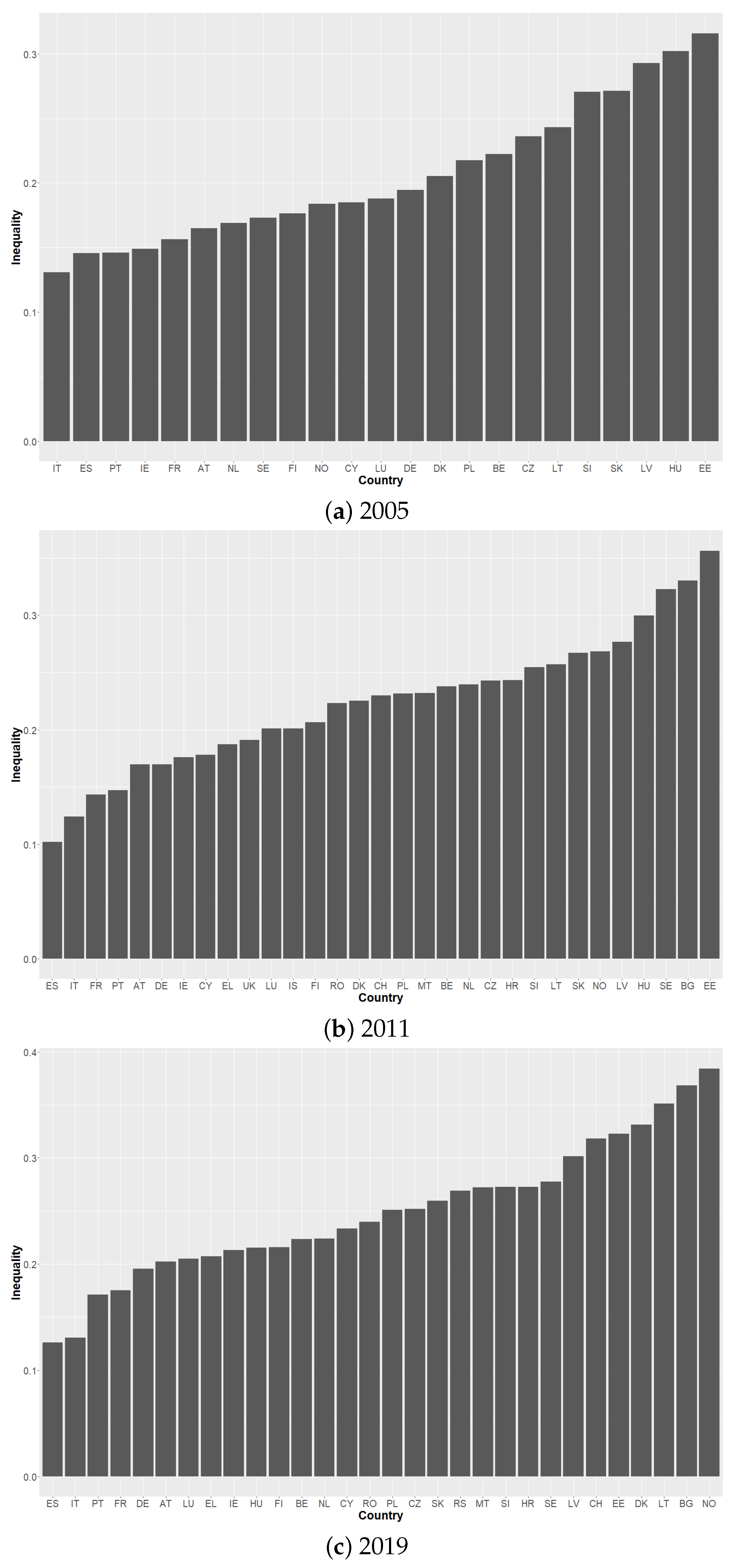
Figure 1 shows the country rankings based on (8) in all three waves. The average IOP is 20% in 2005, 22% in 2011 and 25% in 2019. This means that the average share of opportunity inequality in total inequality across European countries rises from one-fifth in 2005 to one quarter in 2019. Estonia is the most unequal country in terms of opportunity in 2005, with 31% of total inequality explained by unequal past conditions, and it is also the most unequal in 2011 (with a relative IOP value of 35%). In the final wave (2019), it is replaced by Norway. As much as 38% of the total multivariate inequality in income and health in Norway can be attributed to inequality due to parental background, gender and age. Italy and Spain are two countries that are consistently the most equal countries in each wave. They just change positions. In 2005, Italy had the lowest value (13%), whereas in 2011 and 2019, Spain had the lowest relative IOP (10% and 12%, respectively), followed by Italy (12% and 13%, respectively).

Looking at country rankings instead of inequality scores, we see that they change over the waves: considering only countries present in 2005, the rank correlations are 0.77 (2005 vs. 2011) and 0.65 (2005 vs. 2019). The last two waves are more stable, with a rank correlation of 0.81. Let us take a closer look at some countries that have significantly worsened their position between 2005 and 2019. These are Sweden (8th in 2005 and 23rd in 2019)6, Norway (10th in 2005 and 30th in 2019) and Denmark (14th in 2005 and 27th in 2019). This result may seem surprising, as Scandinavia is generally seen as a land of equality, but not when it comes to equality of opportunity, which is also in line with some recent research (Carneiro et al. 2021; Heckman and Landersø 2002). First, these countries are equal in terms of income, but not in terms of health, which is confirmed by our more detailed results: Norway and Denmark were the worst for health opportunity equality in 2019.7 As Heckman and Landersø (2002) show, Scandinavian countries achieve low income inequality through post-redistribution (their tax and transfer programs), but not through pre-redistribution (i.e., improving the human capital of children across generations). They are therefore characterized by significant inequality of opportunity for outcomes such as health or education. Second, these countries are equal in terms of income, but not so much in terms of income opportunity: they occupy middle positions in the ranking of income inequality of opportunity. Kapera et al. (2023) reach a similar conclusion for more outcomes (income, health and education) and a different IOP measure.

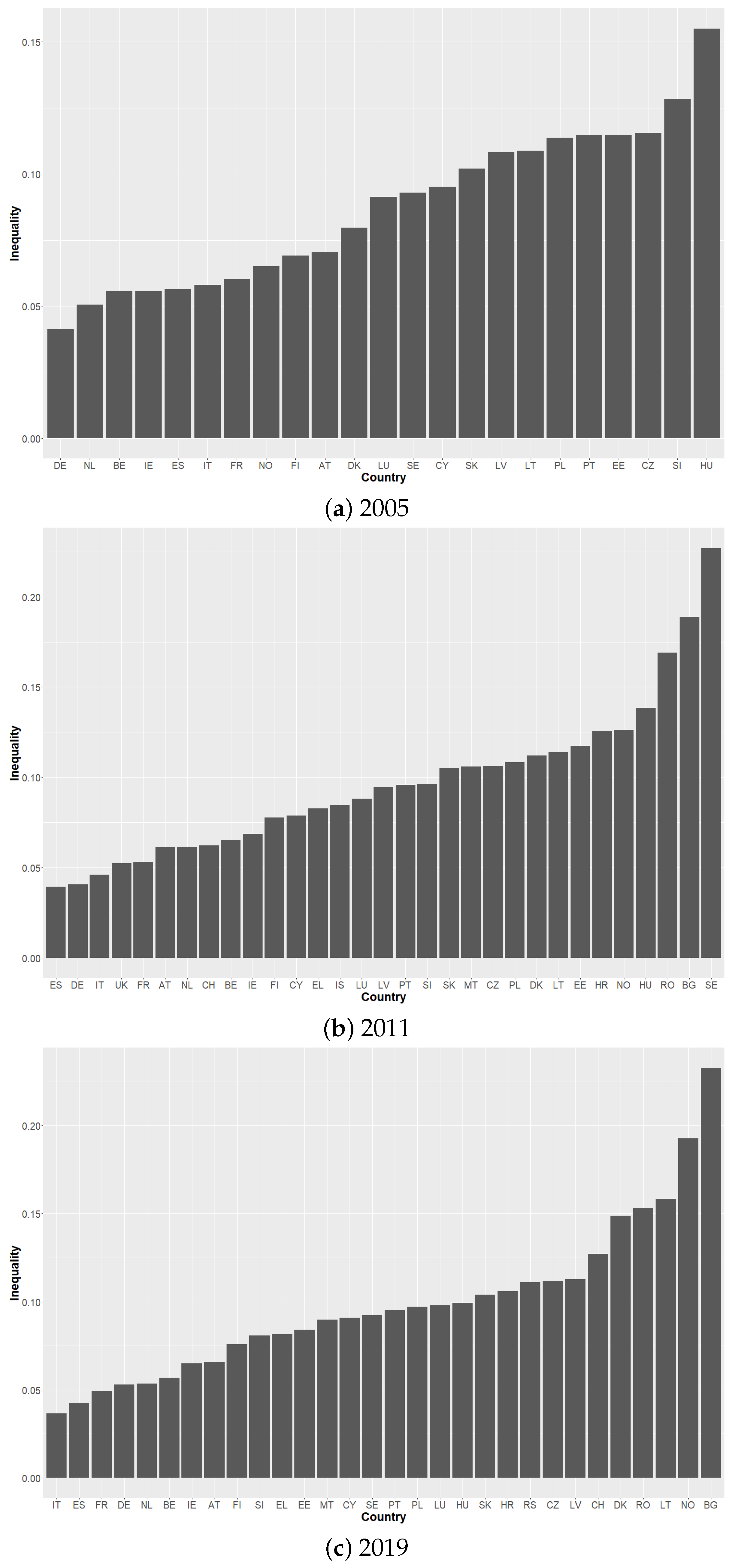
Figure 2 shows the ranking of countries based on the relative MLD index. The average values of the index are 8.6% in 2005, 9.6% in 2011 and 9.8% in 2019, so similar to the average Gini values, there is a slight increase in IOP over the years. Compared to the Gini index, the MLD values are significantly lower, but this is a well-known fact (see, e.g., Brunori et al. 2019). This is because the MLD is very sensitive to extreme values and these are largely removed by smoothing the distribution, so that in terms of overall inequality the MLD is lower than, for example, the Gini. In 2005, the lowest value is for Germany (4%) and the highest for Hungary (15%). In 2011, Germany and the countries that are also the most equal according to Gini, namely Italy and Spain, occupy the lowest IOP positions, with MLD values close to 4%. The highest values are found in Romania (17%), Bulgaria (19%) and Sweden (22%). In 2019, the values range from 3.6% for (again) Italy to 23% for Bulgaria (Figure 2c). Bulgaria also has the second highest value of Gini IOP in 2011. Spain is the second most equal (3.6% for Italy and 4.2% for Spain) and Norway (19%) the second most unequal. For comparison, Checchi et al. (2015) use MLD for the income IOP and obtain a comparable but higher range values for European countries using EU-SILC, i.e., between 2.5% and 30%.

As we can see, the most equal countries are the same for Gini and MLD, but in general, the two measures sometimes diverge. Overall, the rankings induced by the two measures are significantly positively correlated in the last two waves (rank correlations are around 0.77) and less so in 2005 (rank correlation is 0.62). Over the three waves, the Scandinavian countries also move up in the MLD-induced ranking. In 2019, Sweden is the 23rd most unequal country, Denmark the 27th and, as already mentioned, Norway the most unequal country in terms of opportunity. In addition, similar to the results of the Gini index, these countries occupy middle positions in terms of income inequality of opportunity, and Norway and Denmark are the most unequal countries in terms of health opportunity. The inequality scores are different, as might be expected, but the general trends remain the same for both measures.

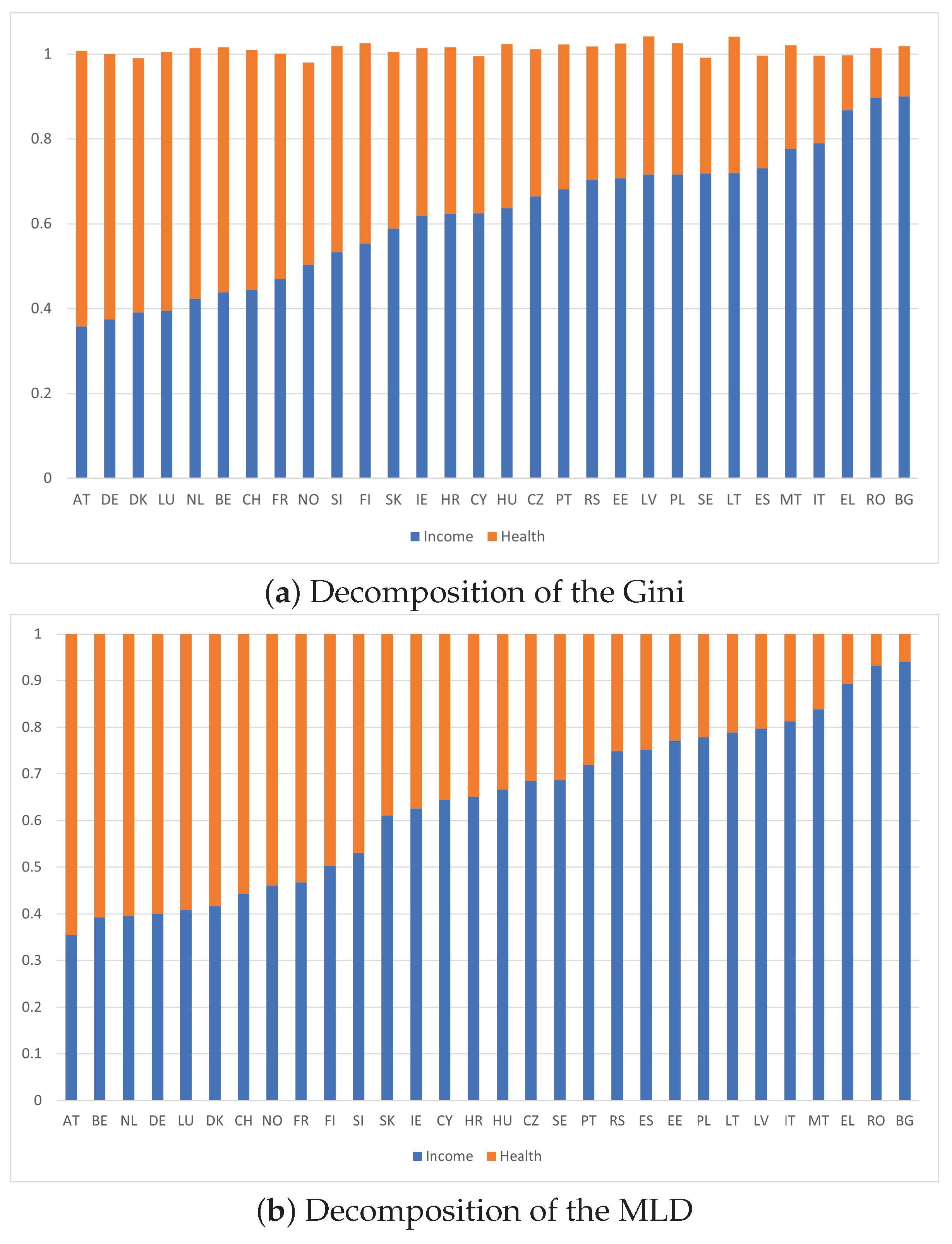
Next, we use our decomposition results, Lemmas 1 and 2. This is shown in Figure 3 for the last wave. It turns out that the impact of dependence measured by $\kappa$ is negligible (no more than 3%, and typically around 1.5%). This does not rule out significant dependence in the original variables at the individual level, which can be largely reduced by smoothing the distribution and does not carry over to the type level. The residual is also very small (typically less than 1%). In Figure 3, we order the countries according to the increasing contribution of income. It is the lowest in Austria (35%) and the highest in Bulgaria (90%). This decomposition is very similar for the MLD index (Figure 3b), both in terms of rankings and values.

The main reference is Kapera et al. (2023), so we attempt to make some comparisons. They also use EU-SILC data, but have more outcomes; in addition to income and health, they also include educational attainment as one of the outcomes. Some qualitative conclusions between their work and ours are similar, such as the above-mentioned observation that the Scandinavian countries are more unequal in terms of opportunity than in terms of income, and that their position has worsened over time. Furthermore, in both studies, Bulgaria and the Baltic countries are also among the most joint-opportunity unequal. In general, however, our results are not directly comparable with theirs, as they do not report relative measures. Moreover, their main measure, and the one they focus on most when describing their results, takes into account inequality within type, which we do not. For these two reasons, we look at the absolute values of our measures ((3) and (5)) and compare them with their “pure between type” measure, which they also report. They generally obtain higher values of inequality for univariate IOP indices. Given that their measure is more sensitive to inequality at the bottom than ours, this suggests more unequal opportunities at the bottom of the distribution for both outcomes considered separately. This explains why the correlation of their joint measure with ours is not perfect and is higher for the MLD (0.81) than for the Gini (0.73), which tends to attenuate more variation in outcomes at the top or bottom of the distribution compared to the MLD (Cowell and Flachaire 2023). However, for both Gini and MLD, the correlation between their rankings and ours is higher for individual dimensions: 0.89 (0.67) and 0.94 (0.70) for income (health) with Gini and MLD, respectively. The fact that the unidimensional rank correlations are significantly higher than the correlations for joint measures most likely indicates the impact of the third outcome (education) in their joint measure. Finally, similar to their case, in our analysis, the unidimensional rankings of the income and health IOPs are very different: for the absolute Gini index, their correlation is 0.27, and for the absolute MLD it is 0.24. This justifies the use of joint measures to obtain an unambiguous ranking of countries.

4. Conclusions

To conclude, we offer a simple way to extend the most popular measures of inequality of opportunity to account for multidimensional outcomes. The measures are not characterized, but characterizations are not very common for measures of inequality of opportunity (with the recent exception of Bosmans and Öztürk 2021), in contrast to inequality measures. We show how our proposed indices can be applied to the data. We calculate inequality of opportunity in joint health and income in Europe. As the most interesting conclusion, with a multivariate measure, some of the countries that appear to be or are equal in terms of income inequality of opportunity are not necessarily equal in terms of joint inequality of opportunity. Furthermore, the comparison between countries differs depending on which outcome is used. The direct implication and recommendation for empirical and policy research is to use multivariate measures, as this resolves the ambiguities associated with treating outcomes separately and, as shown in this paper, may also change our conclusions about which country/region is the most/least equal. The measures we offer have the additional advantage of being decomposable into the contribution of each dimension and (in the case of the Gini index) the contribution of the association of the dimensions. Such a disaggregated view of inequality is often desirable in applications and practical policy issues.

There are some obvious extensions to the current work. We describe two of the most natural. First, the measures are developed for ex ante inequality of opportunity. A natural research step is to develop the multivariate analogues of the Gini and MLD indices in the ex post framework. In the realm of philosophical discourse, there are two main approaches to IOP: the ex ante approach, which involves identifying individual opportunity sets and subsequently devising a method to gauge inequality among these sets; and the ex post approach, where the focus is on initially identifying individual efforts and then measuring the resulting inequality among individuals who exhibit similar levels of effort. Therefore, the ex-ante and ex-post approaches diverge based on when the measurement exercise takes place—either before or after the revelation of individual efforts (or, more broadly, choices). Within the framework of ex post theory, a fundamental unit of analysis is a tranche, defined as a group of individuals sharing the same level of effort. The predominant focus in the literature centers around scenarios where effort remains unobservable, a common occurrence in widely used surveys and databases. In such cases, individual effort is identified using the Romer’s statistical solution (Roemer 1998), a method that involves identifying effort based on its position in the cumulative distribution function of a univariate outcome within a specific type—defined as a set of individuals sharing similar circumstances—to which the individual belongs. This identification method would have to be redefined in a multivariate framework, multivariate tranches constructed and Gini and MLD measures developed on this basis.

Second, in this paper, we implicitly assume that all attributes are cardinal, like income, and in the empirical analysis we treat self-reported health as such. This is still standard practice for health variables, but there is a large body of literature (e.g., Allison and Foster 2004; Kobus 2015) that calls for treating these variables as they are, namely ordinal variables. They consist of several categories (e.g., from very bad to very good health) that are ordered, but the distance between these categories is unknown. Several authors show that cardinalizing such variables, i.e., assigning numbers to categories and thus imposing a scale on the unknown distance between categories, is flawed. In particular, different but valid cardinalizations can lead to different orderings of distributions and to reversals of conclusions, which is obviously undesirable. Therefore, it makes sense to define inequality measures for ordinal data directly on the (discrete) distribution, which is made invariant to monotone rescaling of the data. It would be interesting and important for applications to redefine IOP measures in the context of ordinal data, for example, using the concepts developed by Kobus (2015) who presents a complete theory of measuring inequality for ordinal data. However, with multiple outcomes, it is likely that they are of a different nature, i.e., that some variables are cardinal and some are ordinal. The work of Muller and Trannoy (2012) and Gravel and Moyes (2012), who develop relevant transfer axioms, can then be used to develop the current IOP framework.