Abstract
Non-negative distributions are important tools in various fields. Given the importance of achieving a good fit, the literature offers hundreds of different models, from the very simple to the highly flexible. In this paper, we consider the power–Pareto model, which is defined by its quantile function. This distribution has three parameters, allowing the model to take different shapes, including symmetrical and left- and right-skewed. We provide different distributional characteristics and discuss parameter estimation. In addition to the already-known Maximum Likelihood and Least Squares of the logarithm of the order statistics estimation methods, we propose several additional methods. A simulation study and an application to two datasets are conducted to illustrate the performance of the estimation methods.
1. Introduction
Univariate continuous distributions play a crucial role in modeling real-world phenomena. While well-known distributions like the normal, exponential, and Pareto distributions are commonly used, there is often a need for specialized distributions, to model specific data patterns. One established practice for defining more flexible distributions is through the quantile function (QF)
where represents the cumulative distribution function (CDF) of the random variable X. Thus, if F is strictly increasing, Q and F are inverse functions of each other, and . QFs possess numerous distinct characteristics that are absent in CDFs. We highlight that new and more flexible QFs can be easily constructed from the combination of existing QFs. For example, the product of QFs is still a valid QF.
Since the QF provides all valuable information about the distribution’s shape, several QF models have been proposed in the literature. The symmetric Tukey lambda distribution (Tukey 1960) and its asymmetric version, known as the generalized lambda distribution (Ramberg and Schmeiser 1972), are both defined in terms of their QF. Similarly, the quantile-based skew logistic distribution introduced by Gilchrist (2000) is also defined through its QF. More recently, Sankaran et al. (2016) introduce a new QF resulting from the sum of the QFs of the generalized Pareto and Weibull distributions.
In some cases, the density and distribution functions for distributions expressed through QFs are not available in closed form, except for specific parameter values. However, those functions can be easily computed by numerically inverting the corresponding QF. One significant advantage of these distributions is the simplicity of their QF, which facilitates the generation of random values through the use of uniform random variables and the application of inference procedures based on quantiles.
In this article, we are interested in the power–Pareto distribution introduced in Gilchrist (2000) and further studied in Hankin and Lee (2006). This is a versatile family of distributions for a non-negative random variable, such as income and wealth. This model is formed through the product of the power and Pareto QFs as
where , , and . We write whenever X has the QF in Equation (1). The parameter c is related to the scale, while and control the shape of the distribution. By fixing or restricting some of this distribution’s parameters, we obtain well-known reduced versions. More precisely, if and , then X follows a Pareto (type I) distribution with the QF
and if and , X has a scaled power distribution with the QF
Furthermore, it can be observed that when , X has the well-known log-logistic distribution, which is a special case of Burr (1942) type XII and Dagum (1977) family of distributions (for further details, see Caeiro and Mateus 2024). The case is not considered here, as it results in a degenerate distribution at c. In the literature, the power–Pareto model in Equation (1) is also known as the Davies distribution (Hankin and Lee 2006) or Hankin–Lee distribution (Nair and Vineshkumar 2010). Hankin and Lee (2006) proposed two inference procedures to estimate the parameters c, , and in Equation (1), namely the maximum likelihood and the least squares method for the logged order statistics. Additionally, the authors compare the efficiency of those two estimation methods by comparing their variance. Since maximum likelihood estimators are often severely biased, for small sample sizes, we argue that solely considering the variance of the estimators may not provide a comprehensive assessment of their performance, and thus, it could lead to misleading conclusions. Therefore, the primary goal of this paper is to discuss a broader set of estimation techniques and consider alternative criteria for a more precise and unbiased comparison of the estimators.
The remainder of the paper is organized as follows. In Section 2, we describe various known properties of the power–Pareto model, like probability density and distribution functions, moments, and quantile-based measures. Several inferential procedures for the parameters of the power–Pareto distribution are discussed in Section 3. In Section 4, we conduct Monte Carlo simulations to analyze the performance of the different inferential procedures. In Section 5, we apply the inferential methods to two real datasets, and Section 6 concludes the article.
2. Statistical Properties of the Power–Pareto Distribution
2.1. Functions
From now on, we use to denote the three parameters of the power–Pareto model. The derivative of , denoted as , is known as the quantile density function. For the model in Equation (1), this function is given by
Note that the quantile density function in Equation (2) satisfies the identity
where is the probability density function.
If we exclude the cases where the power–Pareto reduces to the power, the Pareto, or the log-logistic distributions, neither the distribution function nor the density function can be expressed in closed form. Thus, these functions have to be computed through numerical inversion of the QF. Suppose that is the solution of the equation . Then, the CDF can be expressed as , and the density function can be derived from the inverse function rule as
The density at the left tail can be approximated by
Similarly, the right tail density can be approximated by
In addition, we have
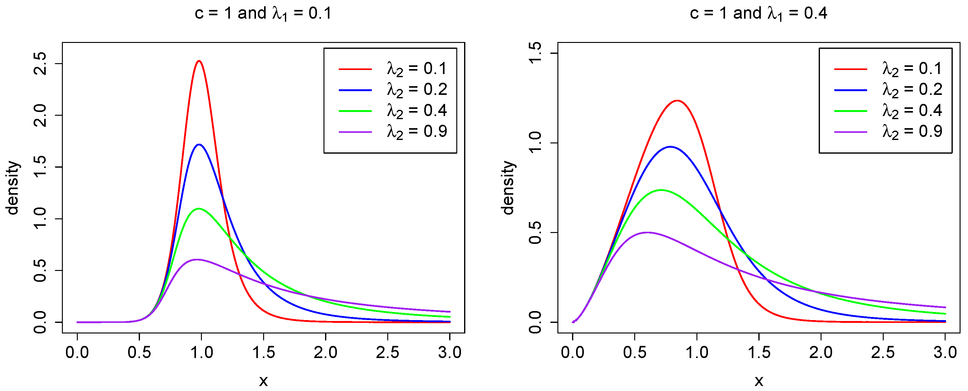
for large x, where is the upper tail index (Finkelstein et al. 2006; Schluter 2018). Hence, the power–Pareto model belongs to the class of heavy-tailed distributions. In numerous applications, it is crucial to estimate accurately the tail index in Equation (6). We refer the reader to Beirlant et al. (2012, 2004); Mehta and Yang (2022); Ndlovu and Chikobvu (2023); Reiss and Thomas (2007), among others. As noted in Hankin and Lee (2006), Equations (4) and (5) show that controls the behavior of the left-hand tail, while governs the right-hand tail. A larger value of results in a shorter left tail, whereas a larger value of leads to a longer right tail. This relationship is illustrated in Figure 1, where different parameter values are used to depict the probability density function.
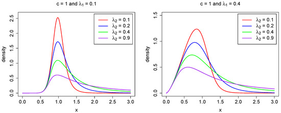
Figure 1.
The density function in (3) for fixed parameters , (left), (right), and selected values for .
2.2. Moments
The k- moment can be expressed in an explicit form as follows:
where , with and , represents the Beta function. Using the notation , the mean () and the variance () are
and exist if and , respectively. Some other measures, like the coefficient of variation (CV), Pearson’s skewness (), and kurtosis () can also be easily obtained in explicit forms,
2.3. Quantile Measures
Quantile-based measures of distributional characteristics, including location, dispersion, skewness, and kurtosis, exhibit less sensitivity to outliers when compared to conventional moments. For the power–Pareto distribution, the median (M) and the interquartile range (IQR) are, respectively, given by
The asymmetry and peakedness of the distribution can be analyzed using Bowley (1901) Skewness () and Moors (1988) Kurtosis () quantile-based coefficients,
and
All the aforementioned quantile-based measures are more robust than moments, since they exist in the complete parameter space, in contrast to moments.
2.4. Order Statistics
Let be a random sample of size n from a population with the QF defined in Equation (1), and let be the corresponding ascending order statistics. Order statistics play a crucial role in statistical inference due to their ability to provide valuable insights into the distribution of X, as well as in estimation procedures for parameters of the model. The density function of is
Note that does not have a closed form, since neither the CDF nor the density function can be expressed in closed form. However, the single moments of the order statistics, , can be easily obtained from the corresponding QF in Equation (1). For the class of distributions in Equation (1), , can be expressed as follows:
Thus, as explicit formulas for moments of order statistics exist, several mathematical quantities associated with order statistics can be derived from Equation (8).
Additional properties can be found in Giorgi and Nadarajah (2010); Nair et al. (2013); Sunoj and Sankaran (2012).
3. Estimation Methods for the Power–Pareto Distribution
In this section, we discuss the parameter estimation methods employed in this paper. For the estimation of the parameters of the aforementioned reduced versions of the power–Pareto model, we refer to Bhatti et al. (2018); Caeiro et al. (2015); Caeiro and Mateus (2023); Lu and Tao (2007); Mateus and Caeiro (2022); Rytgaard (1990); Shakeel et al. (2016); Zaka et al. (2013). Concerning the three-parameter power–Pareto model, in Equation (1), Hankin and Lee (2006) proposed the estimation of the parameters by two methods: maximum likelihood and quantile least squares. The variance–covariance matrix of those two methods is also provided in Hankin and Lee (2006). The maximum likelihood estimators possess desirable asymptotic properties. However, in the case of small samples, this method may exhibit lower efficiency, when compared to other estimation methods. Therefore, in this paper, we consider not only the estimation methods in Hankin and Lee (2006), but also new estimation methods. In the following, let , , …, represent a sample of size n, from the power–Pareto distribution with all three parameters assumed unknown.
3.1. Maximum Likelihood (ML)
The maximum likelihood (ML) estimators of the three parameters are obtained by solving an optimization problem, which involves maximizing the likelihood function, or equivalently, minimizing the negative log-likelihood function. This can be expressed as follows:
where represents the solution of the equation . Here, denotes the ML estimate of .
While the ML estimation method provides asymptotically unbiased estimators and efficiency for large sample sizes, the lack of a closed-form expression for the probability density function requires to be obtained through a three-dimensional numerical search. This makes the ML method computationally intensive, and convergence of the negative log-likelihood to the global minimum can be sensitive to the initial values. Thus, this estimation method for the parameters of the power–Pareto can be computationally complex and challenging, especially for large datasets. Additionally, the ML method can be impacted by model misspecification. Therefore, it is crucial to consider alternative methods, potentially with closed-form expressions for the estimators.
3.2. Log Quantile Least Squares (LQLS)
Hankin and Lee (2006) proposed a regression method for estimating the parameters of the power–Pareto distribution using order statistics. To achieve a simple linear relation involving the parameters, a log transformation is applied, yielding the sum of squares
that needs to be minimized with respect to the vector parameters . Since X is continuous, the inverse probability integral transform guarantees , where U denotes a uniform distribution on the interval . Consequently,
where denotes the -order statistic from a sample of size n from a uniform distribution on . Note that has a Beta distribution with parameters i and . Using Equation (11), we have
with . Thus,
where is the digamma function, the derivative of the log gamma function. For n integer,
where is Euler’s constant. Then, by introducing the notation , Equation (10) can be expressed in matrix form as
where is a column matrix with the logarithm of the order statistics from the sample, , and is an matrix where the row is given by , with . Applying the least squares method, the vector parameters are estimated by
Consequently,
The LQLS method offers several advantages. Firstly, it is more robust against outliers, as the logarithmic transformation reduces the influence of those values. Secondly, unlike the ML method, estimates are based on the order statistics and require straightforward calculations, leading to computational efficiency. However, the LQLS method may exhibit lower efficiency when compared to the ML method and can be sensitive to small sample sizes.
3.3. Percentile (P)
Percentile points were first used for the determination of parameters of the Weibull model (Kao 1959). This method is nowadays popular due to its simplicity. Estimators are found from the relation, through the CDF or the QF, between probabilities and percentile values. To estimate the parameters, one must consider the same number of percentiles. Therefore, given three distinct cumulative probability levels , , and (), the corresponding percentiles, , are the values , , and such that
with Q the QF in Equation (1). Next, applying a log transformation to the ratio between two consecutive percentiles, we obtain
and
Solving the above two equations for and , we obtain
and
Next, we use the following equation for the second percentile:
The estimators are obtained by replacing, in Equations (13)–(15), the percentiles , by the corresponding sample percentiles. A possible choice for the probabilities is . Equivalently, let I be a set of three distinct values from the first n positive integer values, , where n denotes the sample size. Another possible choice of percentiles is , , associated to the cumulative probabilities , where a and b are real constants. A popular choice of the constants is and .
The P method offers simplicity in computation and robustness against outliers. This makes it straightforward to implement and suitable for exploratory analysis and initial estimation, providing a quick and effective way to estimate parameters. However, it may be less efficient and less accurate compared to other methods.
3.4. Least Squares (LS) and Weighted Least Squares (WLS)
Here we consider the difference between the empirical and the theoretical CDF. Then, the least squares (LS) estimator of , denoted by , can be obtained as
Furthermore, the estimation of parameters using the weighted least squares (WLS) method, symbolized as , can be determined by
The LS method involves minimizing the squared difference between the empirical and theoretical CDFs. This method is straightforward to implement and interpret, making it accessible for various applications. However, LS assumes homoscedasticity, which is not valid, since the variance of depends on the index i. This violation does not affect the bias of the estimators, but may increase their variance. On the other hand, the weighting scheme used in the WLS method addresses heteroscedasticity by assigning larger weights to observations that are closer to the center of the sample and smaller weights to observations that are closer to the edges of the sample. Additionally, both the LS and WLS methods are computationally intensive, since both depend on the CDF, which needs to be computed numerically.
3.5. Quantile Least Squares (QLS)
The quantile least squares (QLS) estimator of distribution parameters, denoted by , can be derived by
with defined in Equation (8).
The QLS estimator minimizes the squared difference between the order statistics and their expected value, which can be easily obtained from Equation (8). A limitation of this method is that only exists if ; therefore, the QLS should only be considered if is a small positive value. Furthermore, the accuracy of parameter estimates can be affected by the presence of large outliers.
A weighted version of this method was not considered because it would further restrict its domain of validity.
4. Comparison of the Estimation Methods by Monte Carlo Simulation
In this section, a Monte Carlo simulation study is carried out to compare the performance of the proposed P, LS, WLS, and QLS estimation methods, and to compare them with the ML and LQLS methods, proposed by Hankin and Lee (2006). Davies package was used for the ML method. Parameter estimation with the LS, WLS, and QLS was performed with the R optimization function optim of the R Software version 4.0.0 and using the starting values provided by the davies.start function in Davies package. The power–Pareto distribution was used to generate samples with sizes , 20, 50, 75, and 100. Sample values are generated using the inversion method. In the simulation study, the following parameter combinations were considered:
- Case 1: ;
- Case 2: ;
- Case 3: ;
- Case 4: ;
- Case 5: .
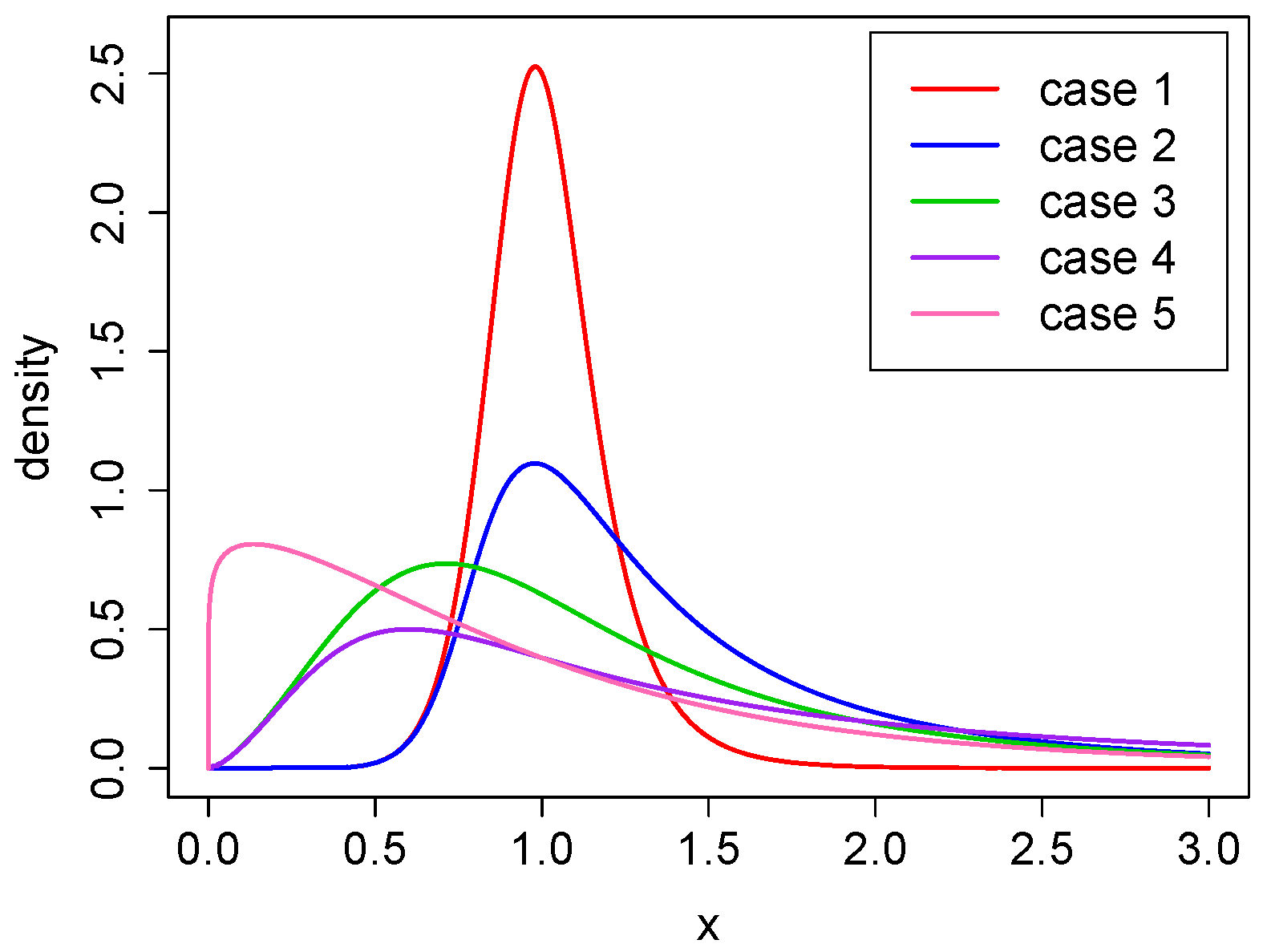
All the parameter combinations provide a power–Pareto distribution with finite mean value and different levels of positive skewness and kurtosis. Both measures increase with respect to and decrease with respect to . The corresponding densities, for all five cases, are presented in Figure 2.

Figure 2.
The density function for cases 1–5.
For each of the three parameters of , denoted generically by , we computed the simulated average bias (ABias), median bias (MBias), and root mean squared error (RMSE) of the corresponding estimator . The statistics are defined by
where is the estimate of computed using the sample.
As a global criterion of comparison, we also computed the average absolute difference between the true and the estimated CDFs,
and the average of the maximum absolute difference between the true and estimated CDFs,
where represents the observation in the sample. The smaller the values of and , the better the fit to the data.
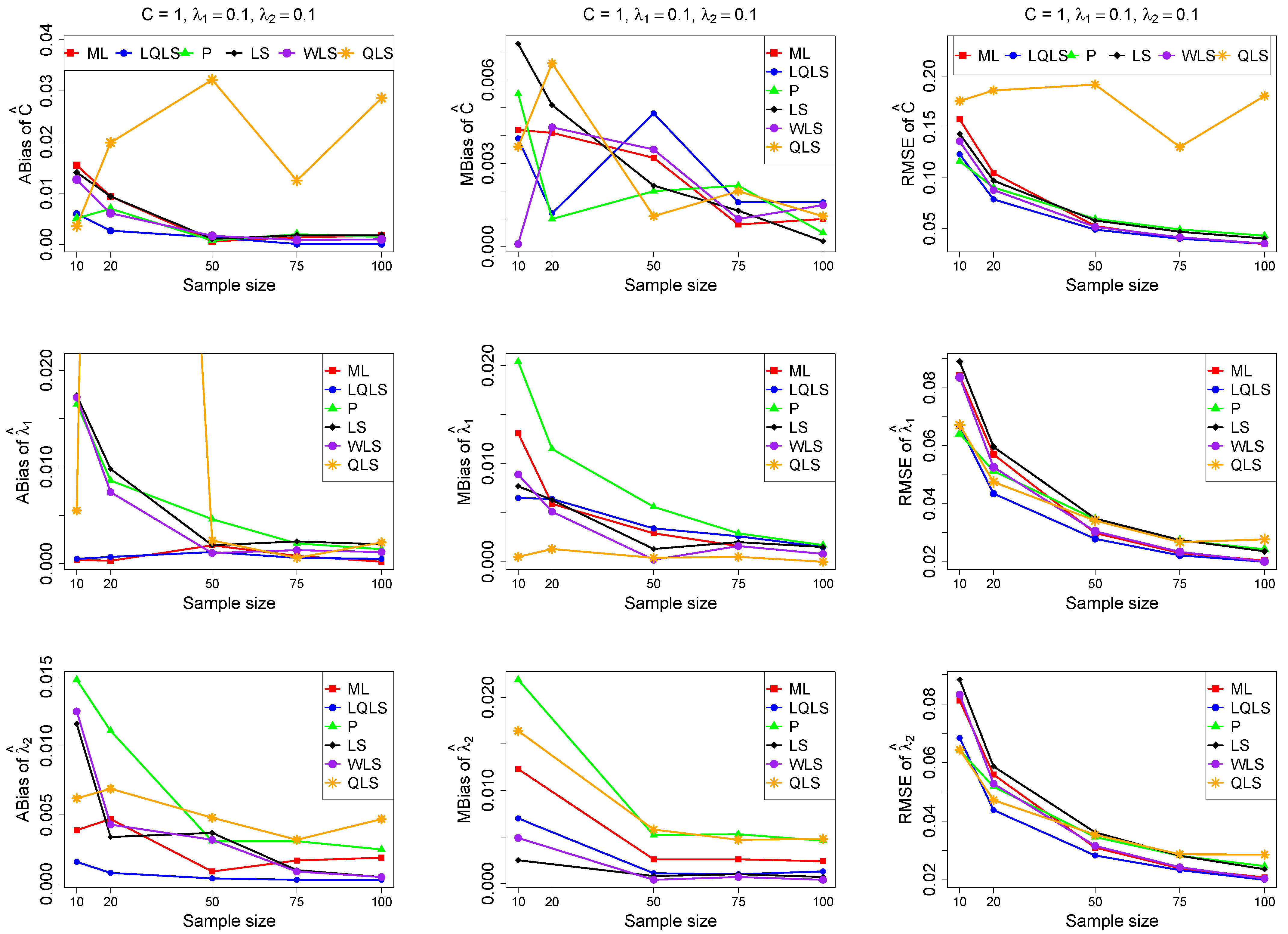
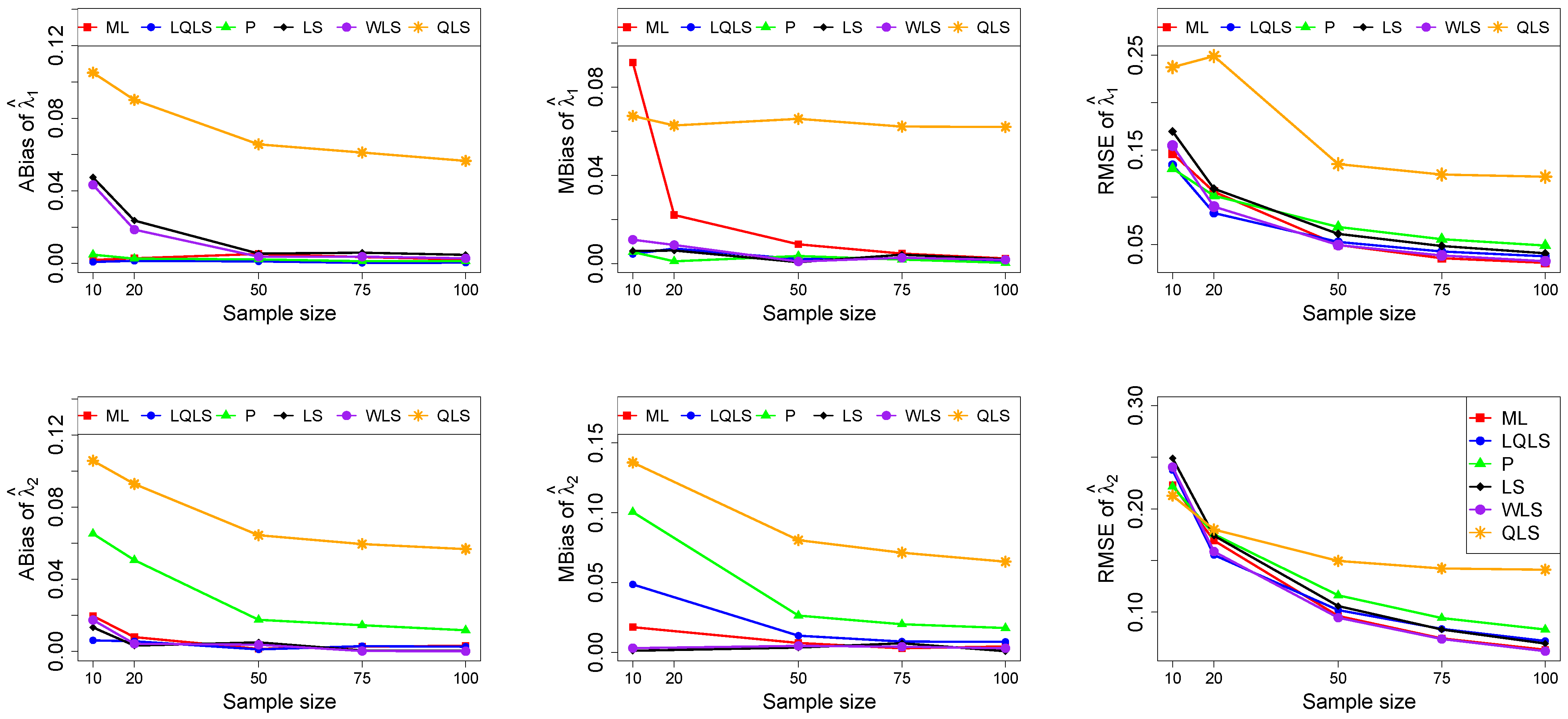
The ABias, MBias, and RMSE are presented in Figure 3, Figure 4, Figure 5, Figure 6 and Figure 7, while the related Table A1, Table A2, Table A3, Table A4 and Table A5, with the corresponding values, are given in Appendix A. It is important to note that it was impossible to obtain estimates provided by the QLS method for a few samples. This was due to the non-convergence of the optimization method used to solve Equation (18). The number of cases where convergence was achieved is indicated beneath each table. This issue is not critical, as the QLS method generally demonstrates the poorest performance. Thus, we do not advise its use.
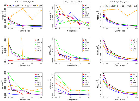
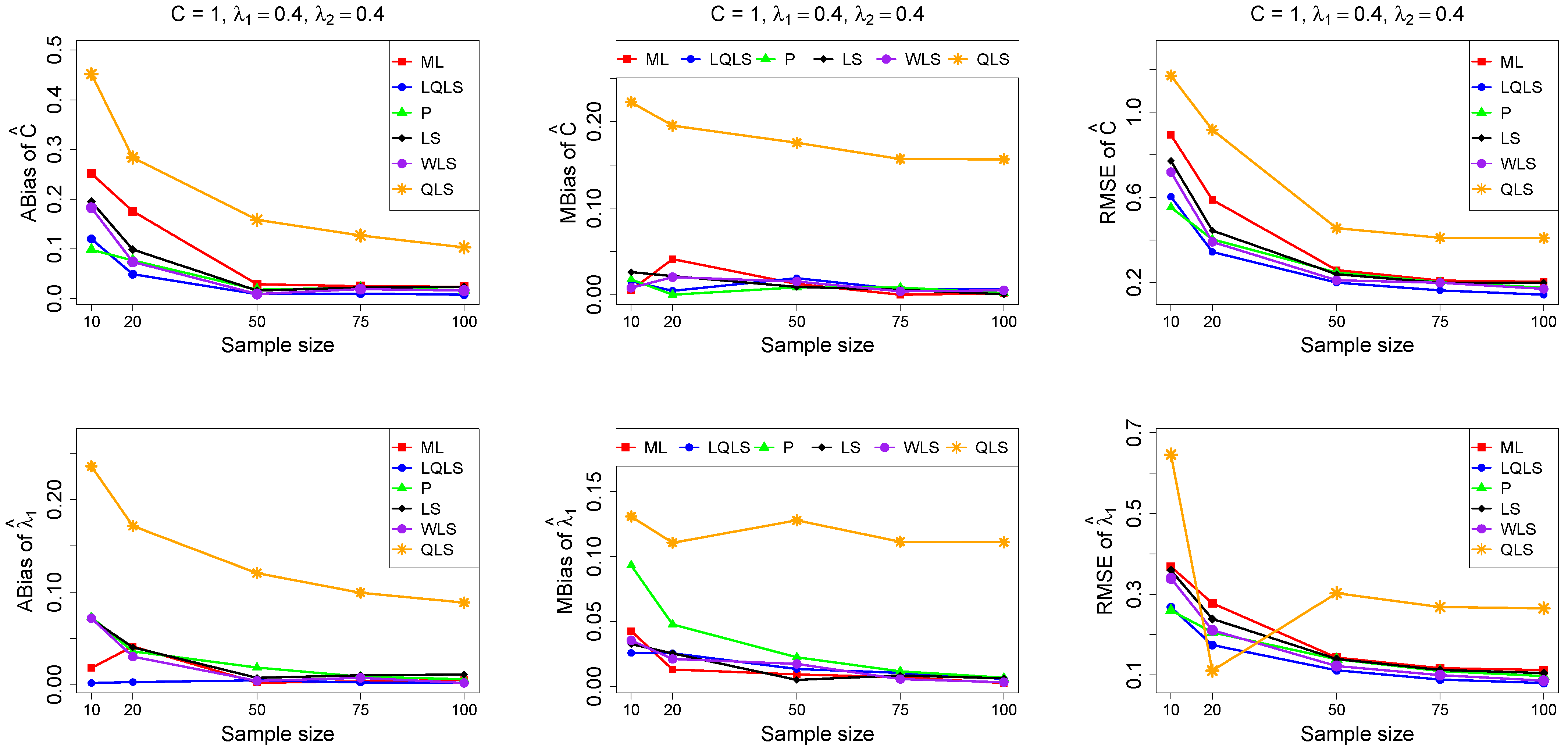
Figure 3.
Monte Carlo simulated ABias, MBias, and RMSE from the power–Pareto distribution with , .

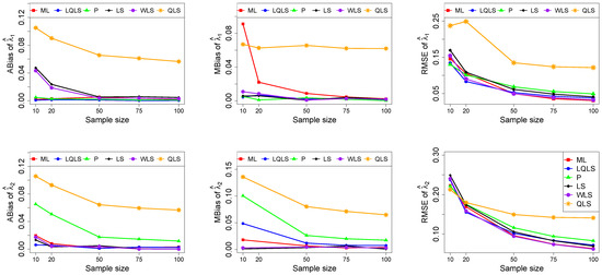
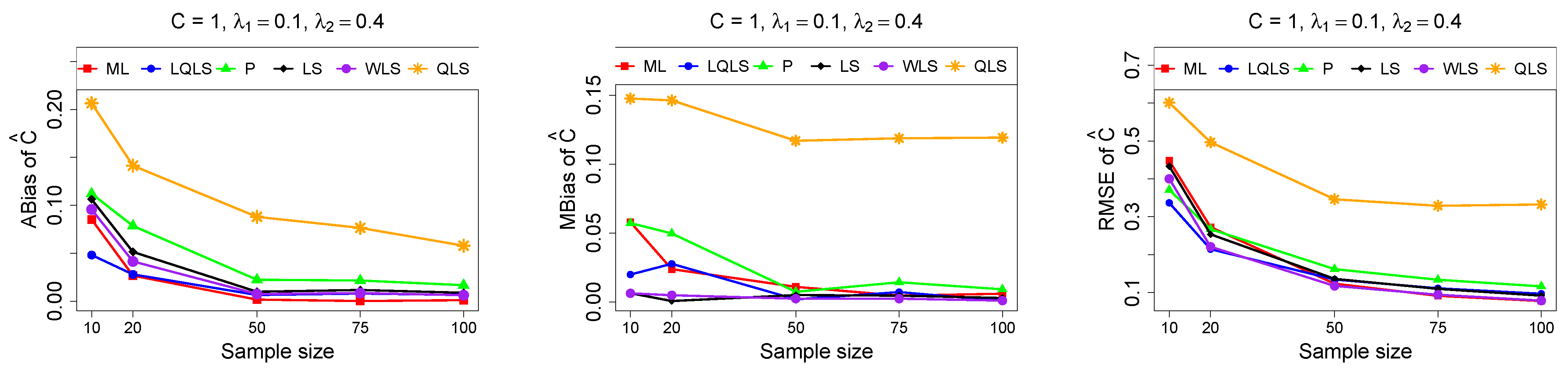
Figure 4.
Monte Carlo simulated ABias, MBias, and RMSE from the power–Pareto distribution with , .
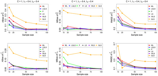
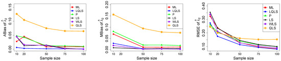
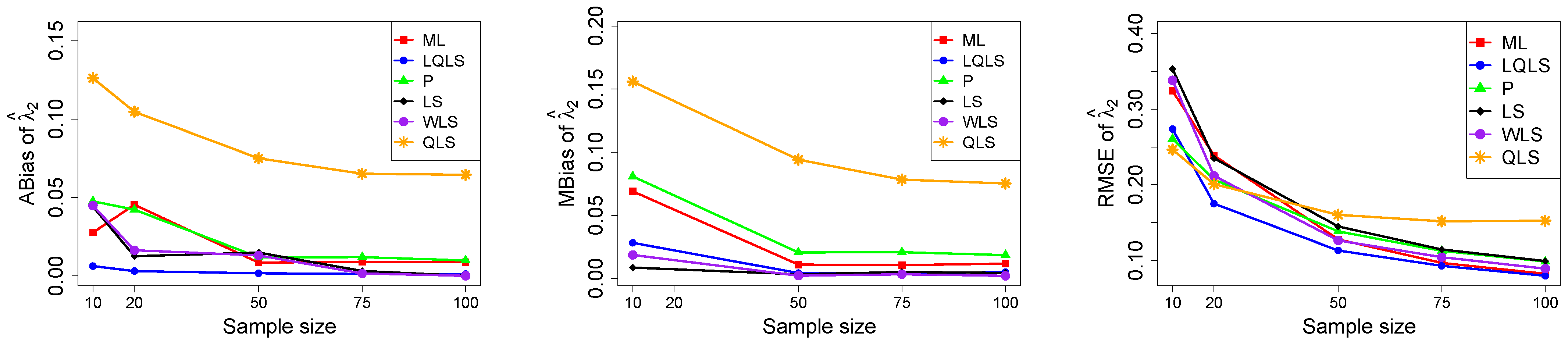
Figure 5.
Monte Carlo simulated ABias, MBias, and RMSE from the power–Pareto distribution with , .
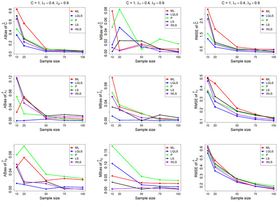
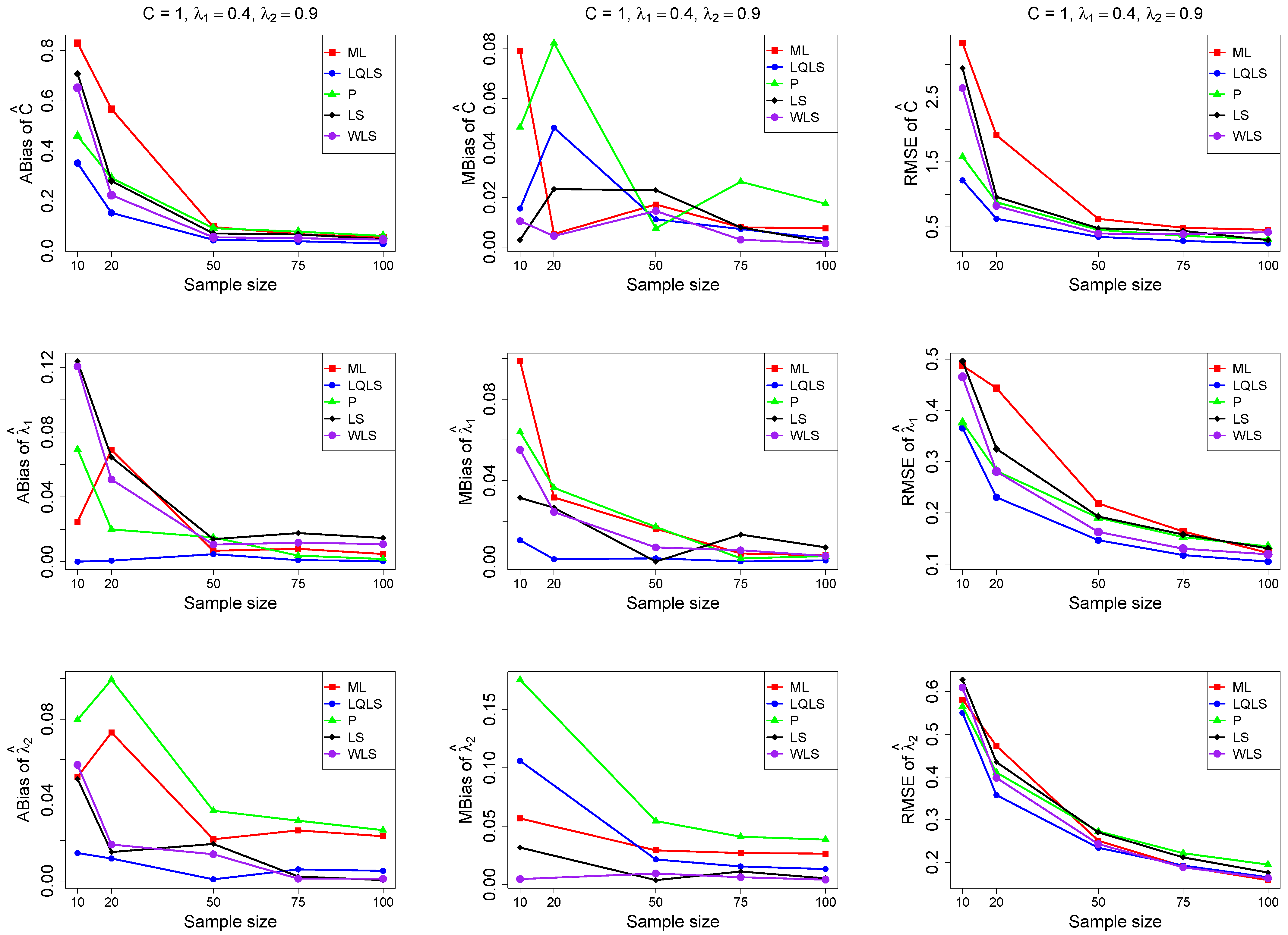
Figure 6.
Monte Carlo simulated ABias, MBias, and RMSE from the power–Pareto distribution with , . Note that we remove the QLS methods because it is out of the range of plot.
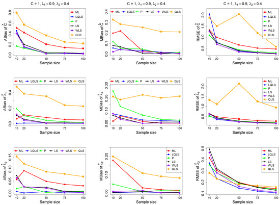
Figure 7.
Monte Carlo simulated ABias, MBias, and RMSE from the power–Pareto distribution with , .
Moreover, since only small sample sizes were considered, it is difficult to assess the convergence of both median and mean simulated bias to zero, likely attributed to sampling error. However, it is evident that if or , the simulated bias is usually closer to zero than if or . In almost all cases, the RMSE of the estimators of the parameters c, , and decreases toward zero, when the sample size increases.
Based on RMSE values in Figure 3, Figure 4, Figure 5, Figure 6 and Figure 7, it is evident that the performance of various estimation methods varies based on the values of and , and also the sample size (n). Regarding the RMSE, we also have the following additional comments:
- For small sample sizes, such as , the P method generally demonstrates the highest efficiency. Moreover, it is not a recommended method for larger sample sizes.
- The WLS method consistently outperforms the LS estimator in estimating each of the three parameters.
- The LQLS method always has a good performance for samples of size . The WLS has a similar performance to the LQLS method if . If , LQLS and WLS methods have a similar performance for .
- The ML method shows strong performance when and and when the sample size is equal to or larger than 50. Thus, we do not recommend its use for samples of size smaller than .
Table 1 and Table 2 provide a comparative analysis of Monte Carlo simulated mean absolute difference and mean maximum absolute difference between true and estimated CDFs. The best values are highlighted in bold. The insights derived from the analysis of these tables can be summarized as follows:

Table 1.
Monte Carlo simulated average absolute difference in Equation (19).
Table 2.
Monte Carlo simulated average of the maximum absolute difference in (20).
- The performance rankings across different methods are consistent between the two tables.
- The WLS methods demonstrate a very good performance, typically yielding the smallest or second smallest values of and .
- The LS method consistently performs slightly worse than WLS, and LQLS shows similar performance to WLS when , except when and . The ML method is never the best performer, but it shows good performance if and or .
- The remaining methods exhibit poor performance. Both P and WLS methods provide generally the largest absolute differences. The exception is the QLS method, for small sample sizes and .
5. Application
In this section, we use two real datasets to illustrate the behavior of the estimators, described in Section 3. To compare the fitted power–Pareto model we computed the Kolmogorov–Smirnov (K-S) statistic and associated p-value for each method. Since parameters are estimated, the p-value of the K-S test is obtained using Monte Carlo simulation. To measure the goodness-of-fit, we also computed the empirical correlation coefficient , between empirical quantiles and the corresponding estimated quantiles , (Beirlant et al. 2004). Since both vectors have monotonically increasing values, will be non-negative.
5.1. Household Income by State in USA
The U.S. Census Bureau defines “household income” as the gross income of all people aged 15 years or older who live in the same housing unit, regardless of their relationship. Household income reflects the standard of living in distinct households and is an important indicator of the local and national economies. Table 3 presents a dataset comprising the median household income in 2016 in the United States, in dollars, of states, as available on the website data.world.1
Table 3.
Household income by state dataset.
The histogram and the boxplot of these observations, in Figure 8, are compatible with the power–Pareto distribution.
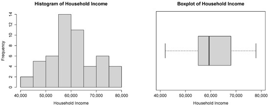
Figure 8.
Histogram and boxplot for the household income dataset.
Table 4 summarizes the estimated parameters, K-S statistics, associated p-values, and the empirical correlation coefficient for various statistical methods applied to the household income dataset.
Table 4.
Parameter estimates under all methods, K-S statistics, and the associated values for the household income data.
Regarding Table 4, it is shown that all estimation techniques produce p-values exceeding , indicating a favorable fit of the power–Pareto distribution. Considering that a lower K-S statistic and a higher p-value signify a better fit, and a higher implies a stronger relationship between observed and expected quantiles, the P method stands out with notably high p-value and , indicating a good fit. Moreover, the LQLS method achieves the highest , further supporting its efficacy. Although the QLS method has a large value, the p-value is the lowest.
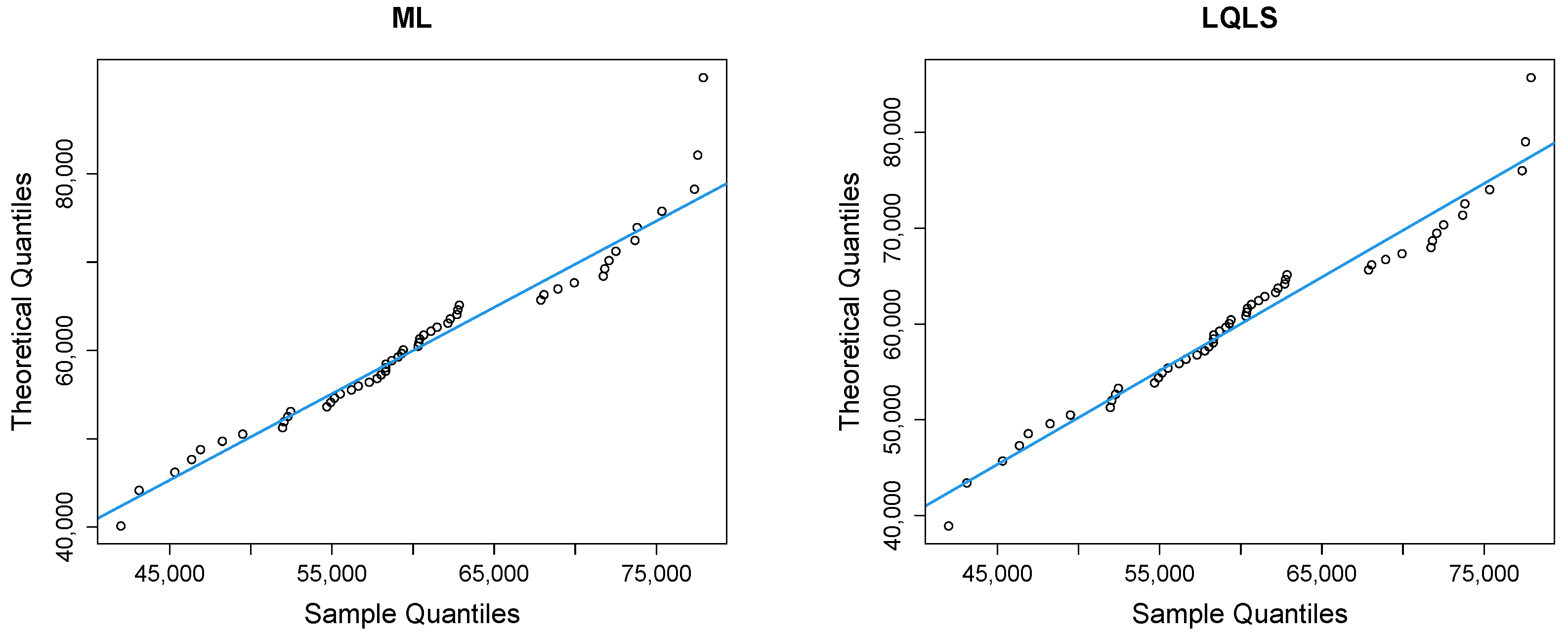
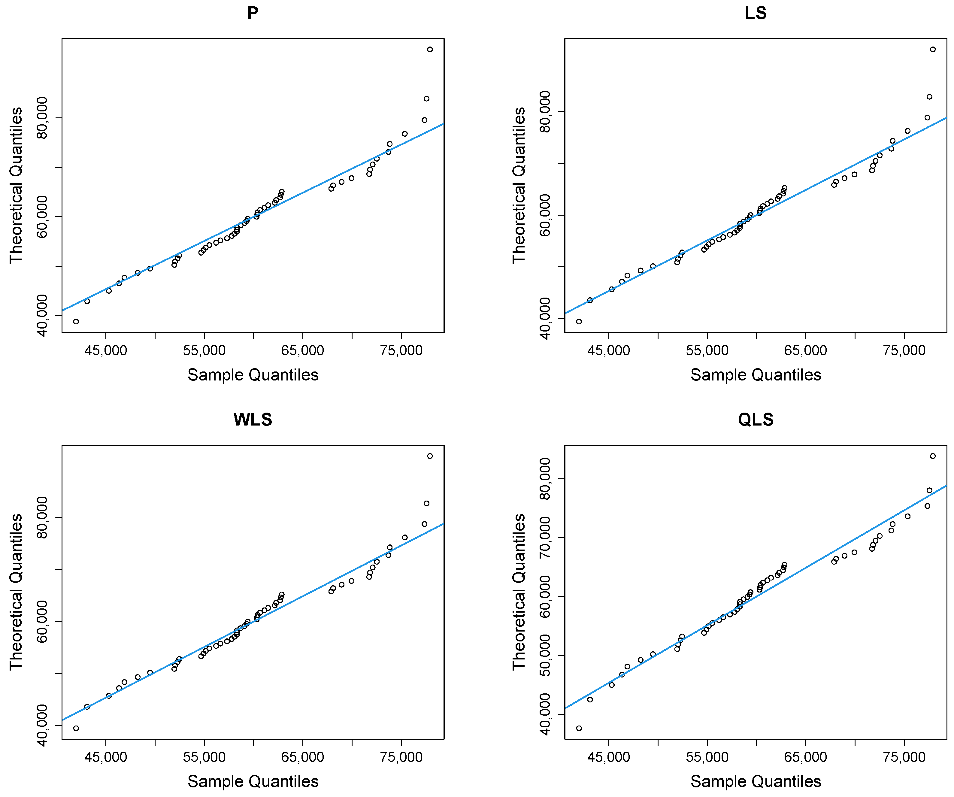
Figure 9 depicts Q-Q plots, comparing the observed data with the estimated quantiles provided from various methods. If the points in the Q-Q plots align closely along the diagonal line, it indicates that the estimated distribution provides an adequate statistical fit. Figure 10 provides the empirical CDF vs. the fitted CDF, for the six different estimation methods.
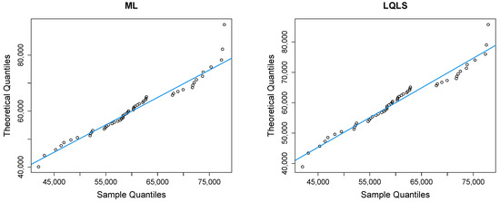
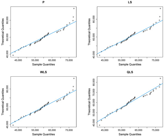
Figure 9.
Q-Q plots of the household income dataset.
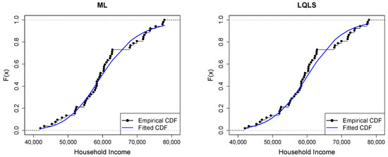
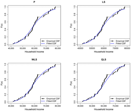
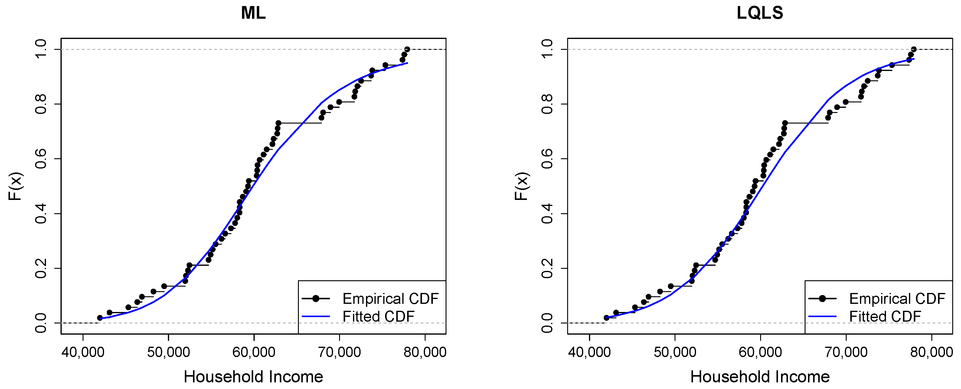
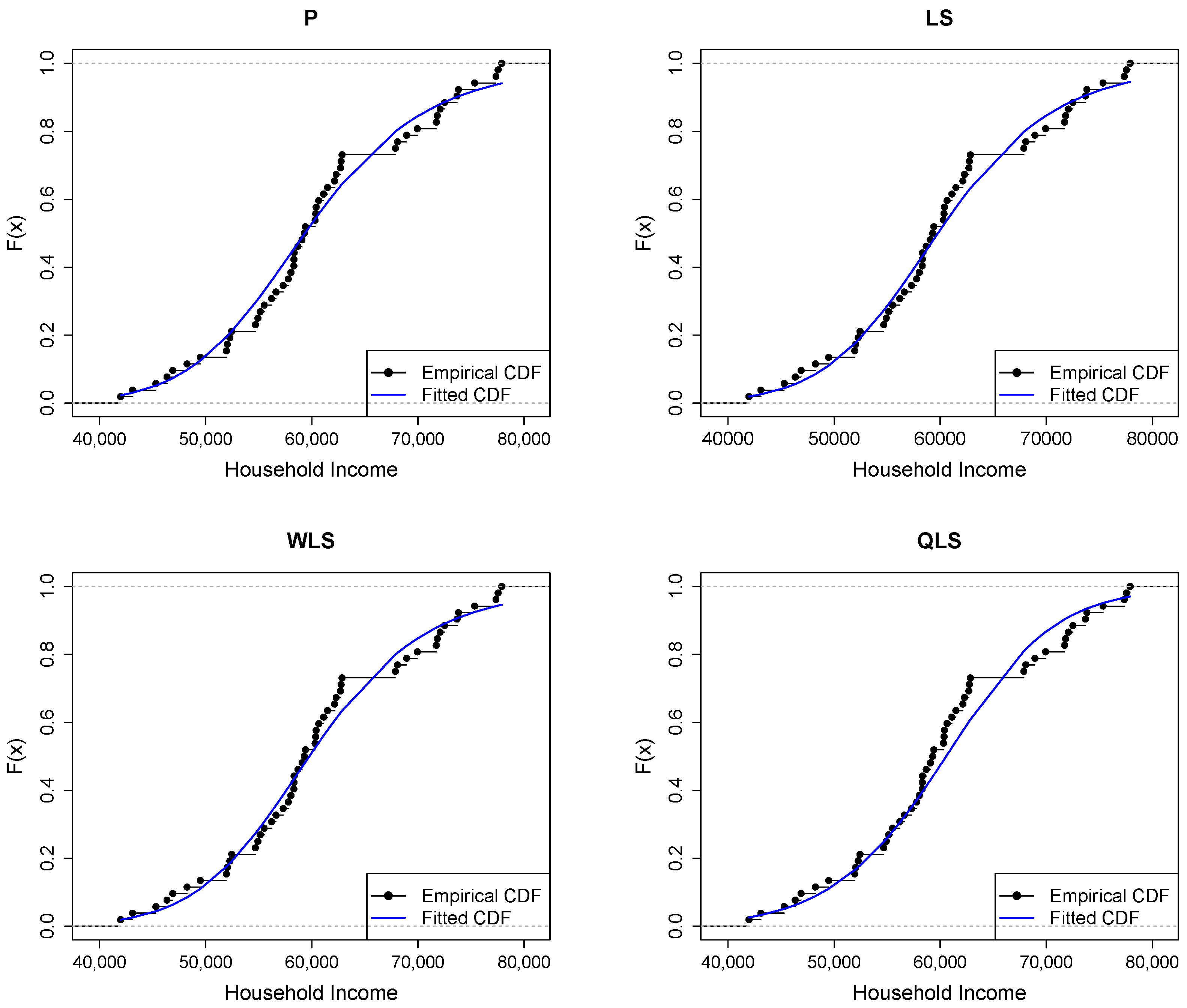
Figure 10.
Empirical vs. fitted CDFs using different estimators for the household income dataset.
Figure 9 shows a good similarity between empirical and fitted quantiles in the body of the distribution, although there are discrepancies in the right tail. All methods provide a good correspondence in the body of the distribution. But the LQLS and QLS methods provide the best correspondence in the right tail. Similar conclusions can be drawn from Figure 10.
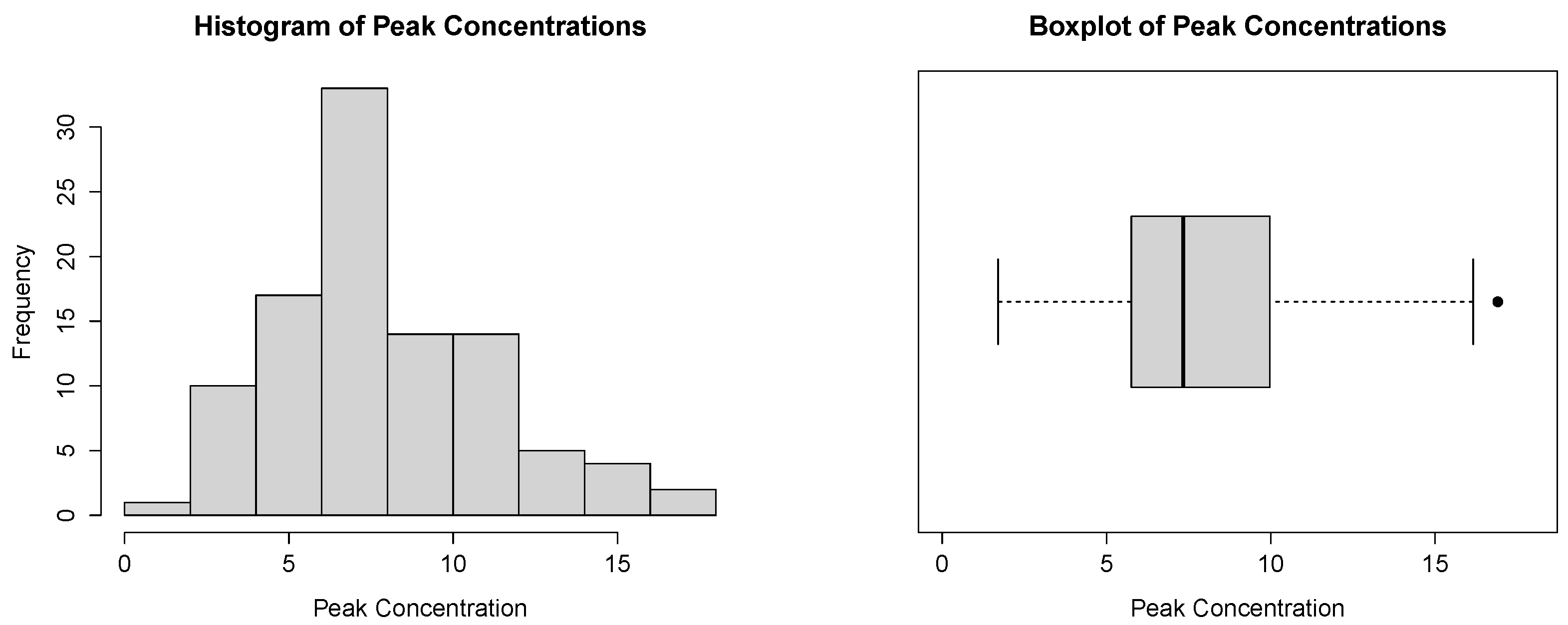
5.2. Peak Concentrations
For the examination of accidental releases of hazardous gases, a method commonly employed is the instantaneous release of a finite volume of gas into a surrounding flow field. Concentration measurements are then taken at a fixed location downwind. In a series of experiments conducted by Hall (1991) involving 100 repetitions, a key parameter for risk assessment was the peak concentrations achieved. The dataset, studied by Hankin and Lee (2006), is provided in Table 5.
Table 5.
Peak concentration dataset.
In Figure 11, we present the histogram and the boxplot of the dataset. Both plots are compatible with the power–Pareto distribution.
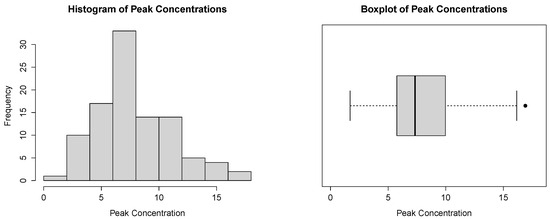
Figure 11.
Histogram and boxplot for the peak concentration dataset.
Table 6 provides the estimated parameters, K-S statistics, the associated p-values, and the empirical correlation coefficient for various statistical methods for the peak concentration dataset.
Table 6.
Parameter estimates under all methods, K-S statistics, and the associated values for the peak concentration dataset.
It is observed that the data conform well to the distribution for all estimation methods, with all associated p-values exceeding and empirical correlation coefficient close to 1. Results for the different estimation methods are similar, except for the QLS, which presents a much higher K-S value. Furthermore, the P, LS, and WLS methods demonstrate favorable outcomes, as indicated by the low K-S statistic, high p-value, and high empirical correlation coefficient, .
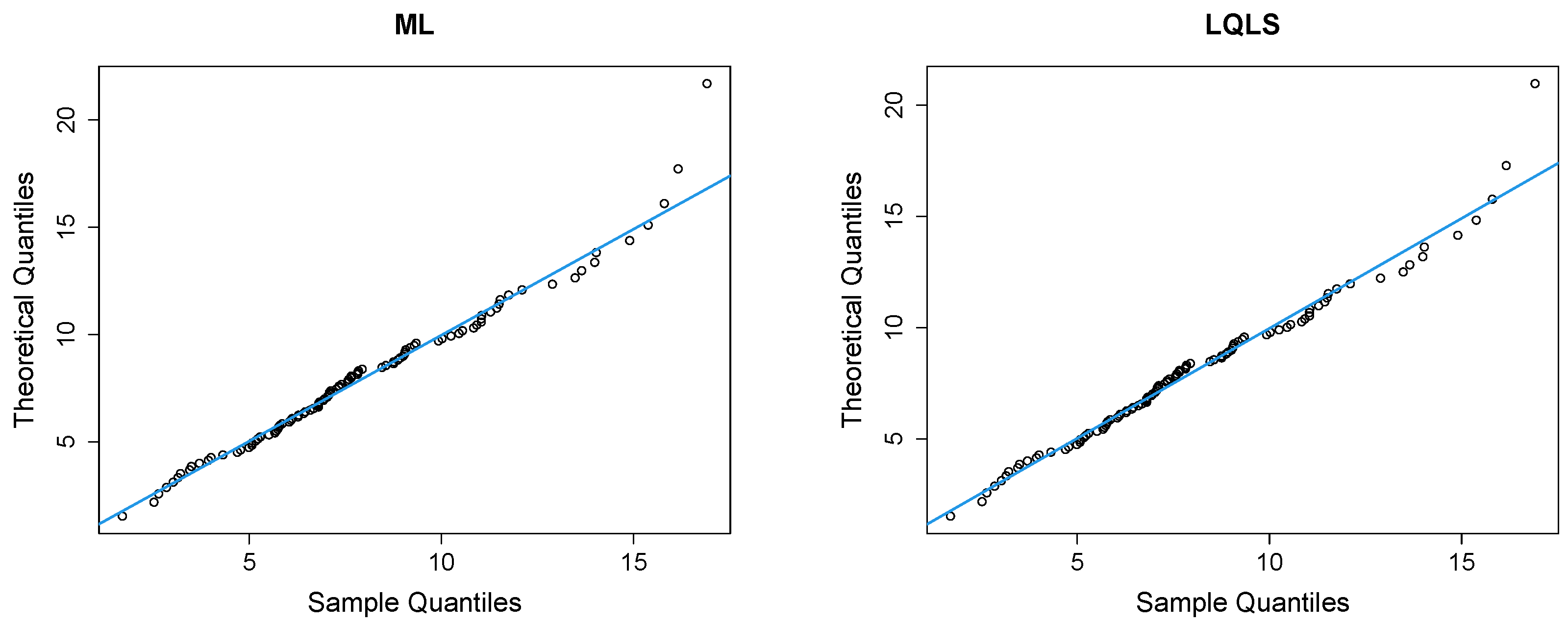
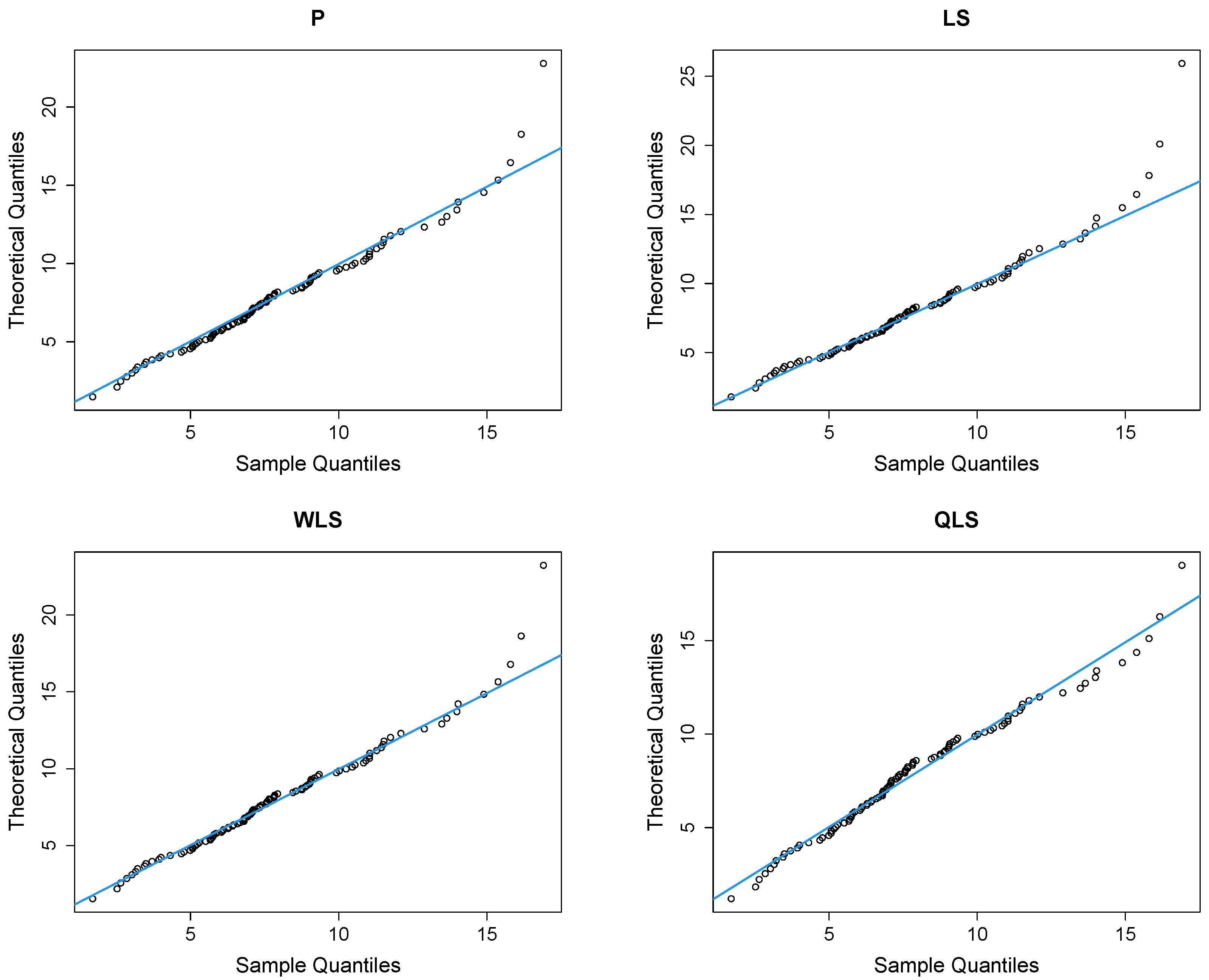
Figure 12 presents Q-Q plots, contrasting the observed data with the estimated quantiles derived from the fitted power–Pareto distribution. Both the P and WLS methods demonstrate a good correspondence, with similar patterns and some discrepancies in the right tail. The QLS again evidences overfitting in the right tail.

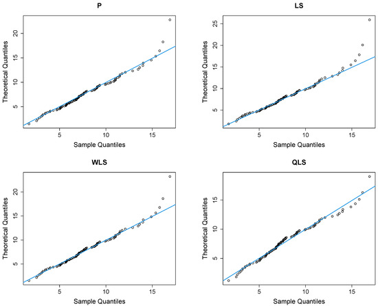
Figure 12.
Q-Q plots of the peak concentration dataset.
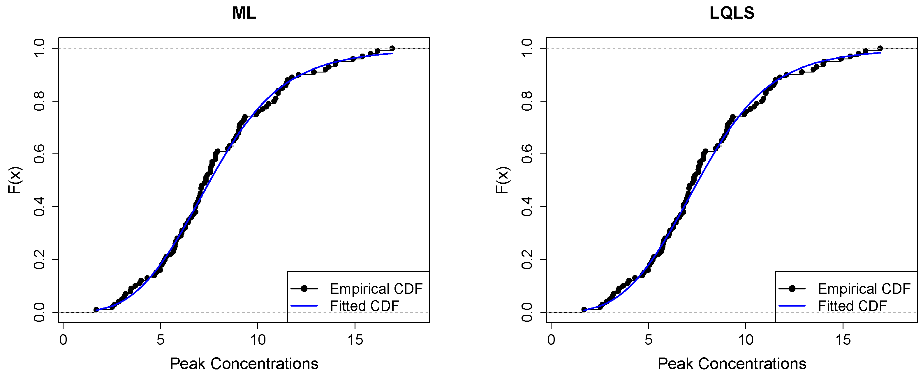
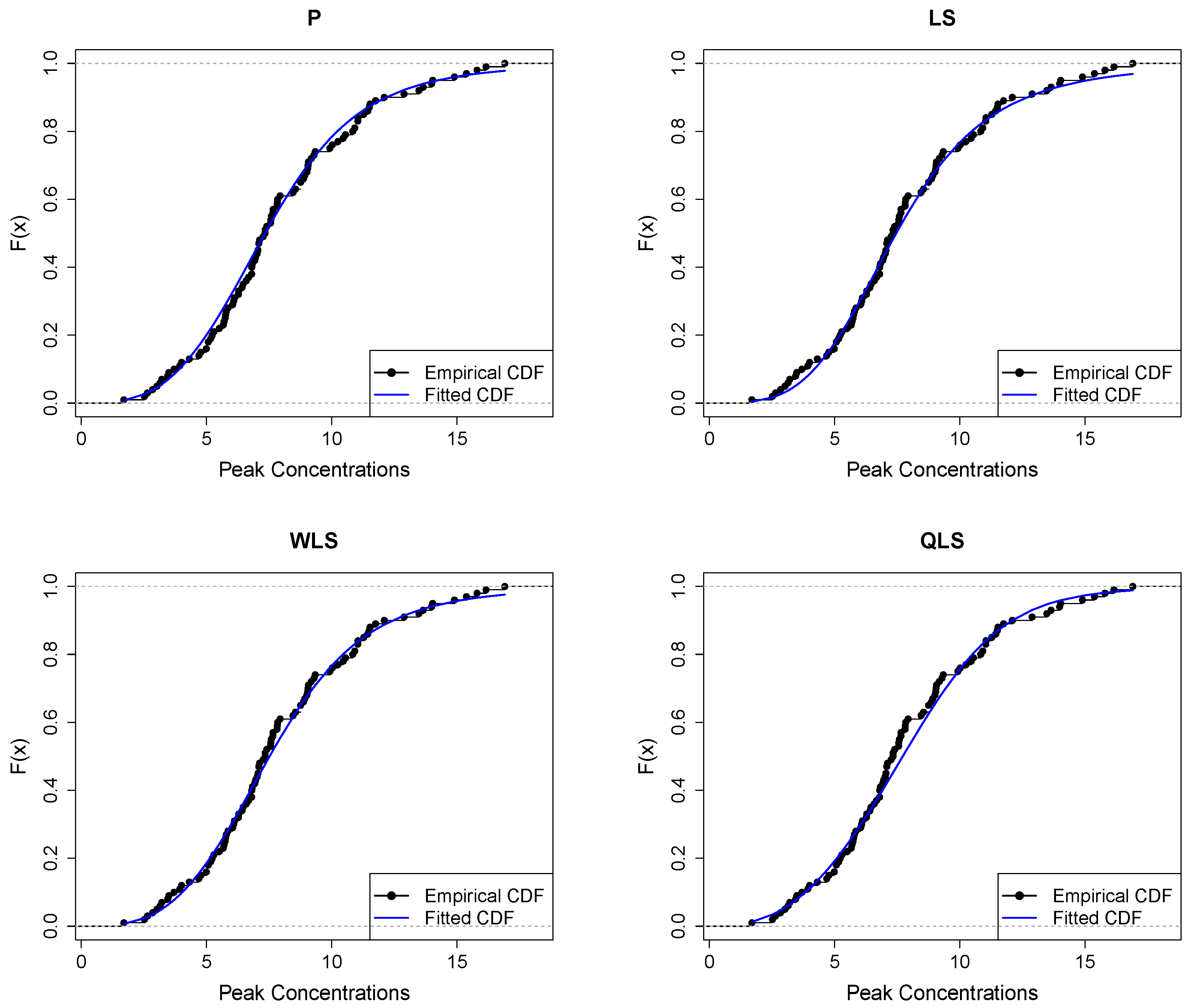
Figure 13 displays the empirical and fitted CDFs. All methods work quite well for analyzing this dataset. However, the P and WLS are the ones that provide the best correspondence between CDFs.
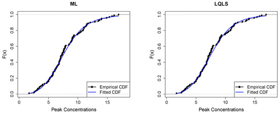
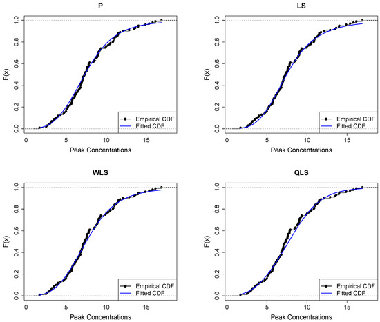
Figure 13.
Empirical vs. fitted CDFs using different estimators for the peak concentration dataset.
6. Conclusions
This study examines the power–Pareto model for non-negative variables. The model has three parameters and can exhibit various shapes, making it suitable for modelling both symmetrical and skewed data. The paper explores distributional characteristics, with a particular focus on different parameter estimation techniques, some of them introduced in this work.
The numerical analysis reveals the importance of selecting an appropriate estimation method based on both sample size and the values of the power–Pareto distribution parameters. Our results indicate that for very small sample sizes, the P method performs well in terms of RMSE. However, for larger sample sizes, the LQLS and WLS methods emerge as adequate choices and are recommended for practical applications.
Additionally, it is worth noting that the ML method also exhibits good performance for larger sample sizes, typically with at least 100 observations. However, it is essential to consider the computational time associated with this method, which is longer when compared to other methods, a factor to weigh in the decision-making process.
Author Contributions
Conceptualization, F.C.; methodology, F.C. and M.N.; software, F.C. and M.N.; validation, F.C.; formal analysis, F.C.; investigation, F.C. and M.N.; data curation, F.C. and M.N.; writing—original draft preparation, M.N.; writing—review and editing, F.C. and M.N.; visualization, F.C. and M.N. All authors have read and agreed to the published version of the manuscript.
Funding
This work is funded by national funds through the FCT—Fundação para a Ciência e a Tecnologia, I.P., under the scope of the projects UIDB/00297/2020 (https://doi.org/10.54499/UIDB/00297/2020, accessed on 6 June 2024) and UIDP/00297/2020 (https://doi.org/10.54499/UIDP/00297/2020, accessed on 6 June 2024) (Center for Mathematics and Applications).
Data Availability Statement
The data supporting the findings in Section 5 of this study are available within the article.
Acknowledgments
The authors thank the referees for their comments and suggestions that led to an improvement of the manuscript.
Conflicts of Interest
The authors declare no conflicts of interest.
Abbreviations
The following abbreviations are used in this manuscript:
| QF | Quantile function |
| CDF | Cumulative distribution function |
| IQR | Interquartile range |
| ML | Maximum Likelihood |
| LQLS | Log quantile least squares |
| P | Percentile |
| LS | Least squares |
| WLS | Weighted least squares |
| QLS | Quantile least squares |
| ABias | Average bias |
| MBias | Median bias |
| RMSE | Root mean squared error |
Appendix A. Monte Carlo Simulation Results
Table A1, Table A2, Table A3, Table A4 and Table A5 provide the ABias, MBias, and RMSE for the cases in Section 4, with the best values highlighted in bold. Figure 3, Figure 4, Figure 5, Figure 6 and Figure 7 are related with these tables.
Table A1.
Monte Carlo simulated ABias, MBias, and RMSE from the power–Pareto distribution with , .
Table A1.
Monte Carlo simulated ABias, MBias, and RMSE from the power–Pareto distribution with , .
| n | ML | LQLS | P | LS | WLS | QLS* | |
|---|---|---|---|---|---|---|---|
| 10 | |||||||
| 20 | |||||||
| 50 | |||||||
| 75 | |||||||
| 100 | |||||||
* The numbers of convergence cases are 983 (n = 10), 978 (n = 20), 966 (n = 50), 985 (n = 75), and 969 (n = 100).
Table A2.
Monte Carlo simulated ABias, MBias, and RMSE from the power–Pareto distribution with , .
Table A2.
Monte Carlo simulated ABias, MBias, and RMSE from the power–Pareto distribution with , .
| n | ML | LQLS | P | LS | WLS | QLS* | |
|---|---|---|---|---|---|---|---|
| 10 | |||||||
| 20 | |||||||
| 50 | |||||||
| 75 | |||||||
| 100 | |||||||
* The numbers of convergence cases are 949 (n = 10), 962 (n = 20), 960 (n = 50), 959 (n = 75), and 952 (n = 100).
Table A3.
Monte Carlo simulated ABias, MBias, and RMSE from the power–Pareto distribution with , .
Table A3.
Monte Carlo simulated ABias, MBias, and RMSE from the power–Pareto distribution with , .
| n | ML | LQLS | P | LS | WLS | QLS* | |
|---|---|---|---|---|---|---|---|
| 10 | |||||||
| 20 | |||||||
| 50 | |||||||
| 75 | |||||||
| 100 | |||||||
* The numbers of convergence cases are 977 (n = 10), 958 (n = 20), 962 (n = 50), 960 (n = 75), and 949 (n = 100).
Table A4.
Monte Carlo simulated ABias, MBias, and RMSE from the power–Pareto distribution with , .
Table A4.
Monte Carlo simulated ABias, MBias, and RMSE from the power–Pareto distribution with , .
| n | ML | LQLS | P | LS | WLS | QLS* | |
|---|---|---|---|---|---|---|---|
| 10 | |||||||
| 20 | |||||||
| 50 | |||||||
| 75 | |||||||
| 100 | |||||||
* The numbers of convergence cases are 913 (n = 10), 936 (n = 20), 941 (n = 50), 946 (n = 75), and 944 (n = 100).
Table A5.
Monte Carlo simulated ABias, MBias, and RMSE from the power–Pareto distribution with , .
Table A5.
Monte Carlo simulated ABias, MBias, and RMSE from the power–Pareto distribution with , .
| n | ML | LQLS | P | LS | WLS | QLS* | |
|---|---|---|---|---|---|---|---|
| 10 | |||||||
| 20 | |||||||
| 50 | |||||||
| 75 | |||||||
| 100 | |||||||
* The numbers of convergence cases are 971 (n = 10), 974 (n = 20), 963 (n = 50), 955 (n = 75), and 967 (n = 100).
Note
| 1 | https://data.world/garyhoov/household-income-by-state (accessed on 6 June 2024). |
References
- Beirlant, Jan, Frederico Caeiro, and M. Ivette Gomes. 2012. An overview and open research topics in statistics of univariate extremes. Revstat–Statistical Journal 10: 1–31. [Google Scholar] [CrossRef]
- Beirlant, Jan, Yuri Goegebeur, Johan Segers, and Jozef L. Teugels. 2004. Statistics of Extremes: Theory and Applications. Chichester: John Wiley & Sons. [Google Scholar] [CrossRef]
- Bhatti, Sajjad Haider, Shahzad Hussain, Tanvir Ahmad, Muhammad Aslam, Muhammad Aftab, and Muhammad Ali Raza. 2018. Efficient estimation of pareto model: Some modified percentile estimators. PLoS ONE 13: e0196456. [Google Scholar] [CrossRef] [PubMed]
- Bowley, Arthur L. 1901. Elements of Statistics. London: PS King & Son. [Google Scholar] [CrossRef]
- Burr, Irving W. 1942. Cumulative frequency functions. The Annals of Mathematical Statistics 13: 215–32. [Google Scholar] [CrossRef]
- Caeiro, Frederico, Ana P. Martins, and Inês J. Sequeira. 2015. Finite sample behaviour of classical and quantile regression estimators for the pareto distribution. In AIP Conference Proceedings. New York: AIP Publishing LLC. [Google Scholar] [CrossRef]
- Caeiro, Frederico, and Ayana Mateus. 2023. A new class of generalized probability-weighted moment estimators for the pareto distribution. Mathematics 11: 1076. [Google Scholar] [CrossRef]
- Caeiro, Frederico, and Ayana Mateus. 2024. Reduced bias estimation of the shape parameter of the log-logistic distribution. Journal of Computational and Applied Mathematics 436: 115347. [Google Scholar] [CrossRef]
- Dagum, Camilo. 1977. A new model for personal income distribution: Specification and estimation. Economie Appliqué 30: 413–37. [Google Scholar] [CrossRef]
- Finkelstein, Mark, Howard G. Tucker, and Jerry Alan Veeh. 2006. Pareto tail index estimation revisited. North American Actuarial Journal 10: 1–10. [Google Scholar] [CrossRef]
- Gilchrist, Warren. 2000. Statistical Modelling with Quantile Functions. Boca Raton: Chapman & Hall/CRC. [Google Scholar] [CrossRef]
- Giorgi, Giovanni Maria, and Saralees Nadarajah. 2010. Bonferroni and gini indices for various parametric families of distributions. METRON 68: 23–46. [Google Scholar] [CrossRef]
- Hall, David J. 1991. Repeat Variability in Instantaneously Released Heavy Gas Clouds–Some Wind Tunnel Experiments. Technical report LR 804 (PA). Stevenage: Warren Spring Laboratory. [Google Scholar]
- Hankin, Robin K. S., and Alan Lee. 2006. A new family of non-negative distributions. Australian & New Zealand Journal of Statistics 48: 67–78. [Google Scholar] [CrossRef]
- Kao, John H. K. 1959. A graphical estimation of mixed weibull parameters in life-testing of electron tubes. Technometrics 1: 389–407. [Google Scholar] [CrossRef]
- Lu, Hai-Lin, and Shin-Hwa Tao. 2007. The estimation of pareto distribution by a weighted least square method. Quality & Quantity 41: 913–26. [Google Scholar] [CrossRef]
- Mateus, Ayana, and Frederico Caeiro. 2022. Improved shape parameter estimation for the three-parameter log-logistic distribution. Computational and Mathematical Methods 2022: 8400130. [Google Scholar] [CrossRef]
- Mehta, Navya Jayesh, and Fan Yang. 2022. Portfolio optimization for extreme risks with maximum diversification: An empirical analysis. Risks 10: 101. [Google Scholar] [CrossRef]
- Moors, Johannes Josephus Antonius. 1988. A quantile alternative for kurtosis. Journal of the Royal Statistical Society: Series D (The Statistician) 37: 25–32. [Google Scholar] [CrossRef]
- Nair, Narayanan Unnikrishnan, and Balakrishnapillai Vineshkumar. 2010. L-moments of residual life. Journal of Statistical Planning and Inference 140: 2618–31. [Google Scholar] [CrossRef]
- Nair, Narayanan Unnikrishnan, Paduthol Godan Sankaran, and Narayanaswamy Balakrishnan. 2013. Quantile-Based Reliability Analysis. New York: Springer. [Google Scholar] [CrossRef]
- Ndlovu, Thabani, and Delson Chikobvu. 2023. The generalised pareto distribution model approach to comparing extreme risk in the exchange rate risk of bitcoin/us dollar and south african rand/us dollar returns. Risks 11: 100. [Google Scholar] [CrossRef]
- Ramberg, John S., and Bruce W. Schmeiser. 1972. An approximate method for generating symmetric random variables. Communications of the Association for Computing Machinery 15: 987–90. [Google Scholar] [CrossRef]
- Reiss, Rolf-Dieter, and Michael Thomas. 2007. Statistical Analysis of Extreme Values with Applications to Insurance, Finance, Hydrology and Other Fields. Basel: Birkhäuser Verlag. [Google Scholar] [CrossRef]
- Rytgaard, Mette. 1990. Estimation in the pareto distribution. ASTIN Bulletin: The Journal of the IAA 20: 201–16. [Google Scholar] [CrossRef]
- Sankaran, Paduthol Godan, Narayanan Unnikrishnan Nair, and Narayanan Nellikkattu Midhu. 2016. A new quantile function with applications to reliability analysis. Communications in Statistics-Simulation and Computation 45: 566–82. [Google Scholar] [CrossRef]
- Schluter, Christian. 2018. Top incomes, heavy tails, and rank-size regressions. Econometrics 6: 10. [Google Scholar] [CrossRef]
- Shakeel, Muhammad, Muhammad Ahsan ul Haq, Ijaz Hussain, Alaa Mohamd Abdulhamid, and Muhammad Faisal. 2016. Comparison of two new robust parameter estimation methods for the power function distribution. PLoS ONE 11: e0160692. [Google Scholar] [CrossRef] [PubMed]
- Sunoj, Sreenarayanapurath Madhavan, and Paduthol Godan Sankaran. 2012. Quantile based entropy function. Statistics & Probability Letters 82: 1049–53. [Google Scholar] [CrossRef]
- Tukey, John Wilder. The Practical Relationship between the Common Transformations of Percentages and Counts and of Amounts. Technical Report 36. Princeton: Statistical Techniques Research Group, Princeton University.
- Zaka, Azam, Navid Feroze, and Ahmad Saeed Akhter. 2013. A note on modified estimators for the parameters of the power function distribution. International Journal of Advanced Science and Technology 59: 71–84. [Google Scholar] [CrossRef]


Disclaimer/Publisher’s Note: The statements, opinions and data contained in all publications are solely those of the individual author(s) and contributor(s) and not of MDPI and/or the editor(s). MDPI and/or the editor(s) disclaim responsibility for any injury to people or property resulting from any ideas, methods, instructions or products referred to in the content. |
© 2024 by the authors. Licensee MDPI, Basel, Switzerland. This article is an open access article distributed under the terms and conditions of the Creative Commons Attribution (CC BY) license (https://creativecommons.org/licenses/by/4.0/).