Success at the Summer Olympics: How Much Do Economic Factors Explain?

Abstract

Many econometric analyses have attempted to model medal winnings as dependent on per capita GDP and population size. This approach ignores the size and composition of the team of athletes, especially the role of female participation and the role of sports culture, and also provides an inadequate explanation of the variability between the outcomes of countries with similar features. This paper proposes a model that offers two substantive advancements, both of which shed light on previously hidden aspects of Olympic success. First, we propose a selection model that treats the process of fielding any winner and the subsequent level of total winnings as two separate, but related, processes. Second, our model takes a more structural angle, in that we view GDP and population size as inputs into the “production” of athletes. After that production process, those athletes then compete to win medals. We use country-level panel data for the seven Summer Olympiads from 1988 to 2012. The size and composition of the country’s Olympic team are shown to be highly significant factors, as is also the past performance, which generates a persistence effect.

1. Introduction

This paper contributes to the literature on Olympic success by proposing an econometric specification that accommodates several previously-neglected features of data on medal winnings. Specifically, our proposed model offers two substantive advancements. First, we propose a selection model that treats the process of fielding any winner and the subsequent level of total winnings as two separate, but related, processes. This selection setup is designed to accommodate a salient feature of Olympic data: The majority of participating countries fail to win even a single medal. Previous studies have addressed this data feature using a variety of formal count models and Tobit specifications. Instead, we argue that the data generating process of medal winnings more closely resembles a selection model, which is an extension of a standard two-part model, which is, in turn, an extension of the Tobit setup.

Second, we depart from previous studies, which have emphasized reduced form models intended to generate predictions of medal winnings. Instead, we develop a structural model that attempts to shed light on the channels through which a country “produces” winners. Specifically, previous studies have generated accurate predictions of medal winnings using only a handful of variables, most importantly per capita GDP (PCGDP) and population size. Yet despite the predictive power of those two variables, PCGDP and population size do not appear on the actual field of play, and therefore, neither is directly responsible for medal winnings. Furthermore, neither PCGDP nor population size changes during the two weeks of Olympic competitions, and thus, in an econometric sense, both are predetermined with respect to medal winnings. Our model takes a more structural angle, in that we view PCGDP and population size as inputs into the “production” of athletes. After that production process, those athletes then compete to win medals.

Although we demonstrate the overall fit of our model, our two econometric innovations—using a selection setup and incorporating structural channels—are not designed to provide improved predictions of medal winnings. Indeed, the existing literature already produces impressive fits. Rather, our two innovations seek to shed light on previously under-appreciated aspects of Olympic success. First, our model reveals evidence of significant selection effects, which indicates that the means by which a country fields any medal winner is unique from the process that governs how many total medals that country wins. This finding corroborates previously-reported evidence that, although sending athletes to compete is not prohibitively expensive, producing winners does require considerable resources. Second, our structural approach, in which PCGDP and population size produce athletes who then proceed to compete for medals, provides a more economic interpretation of medals winnings. Such an interpretation does not surface in more prediction-motivated reduced form models.

In addition to our selection/structural details, our model also seeks to address the reality that socioeconomic explanatory variables inevitably leave the performance of some countries, especially those that perform at a level higher than predicted by their economic and demographic characteristics, unexplained. For example, Krishna and Haglund [1] ask: “Why do 10 million Indians win less than one-hundredth of one Olympic medal, while 10 million Uzbeks won 4.7 Olympic medals?” To that end, in addition to accounting for country-specific traits, we also accommodate unmeasured country-specific heterogeneity using two different approaches. The first follows the panel literature by incorporating unobserved country-specific traits that remain (nearly) fixed over time. The second employs a dynamic setup to accommodate that fact that a country’s medal winnings tend to show intertemporal persistence.

Existing studies, while employing mostly reduced-form statistical methods, examine various measures of Olympic success. Some focus on medal counts [2,3,4,5], while other studies examine a country’s total medals expressed as a share of all available medals [6,7,8]. Another branch of literature employs methods more commonly used to study firm efficiency, including data envelope analysis [9,10] and stochastic frontier analysis [11]. All of these cited studies point to considerable variation in country-level performance, which implies the presence of unobserved country-specific traits, such as sports culture, elite sports institutes, sports management, and sports medicine in generating success [12,13,14,15,16].

2. Data

With rare exceptions, such as during the Second World War, the modern summer games have been held every four years since 1896. However, the games have evolved and expanded, both in terms of scale (the number of events included) and in terms of participation (the number of countries represented). While the number of participating countries has increased overall, on occasion political events have affected participation of key countries. For example, the United States and several other countries did not participate in 1980 and the Soviet Union did not participate in 1984. The break up of the former Soviet Union in the late 1980s and early 1990s, and German unification in the early 1990s and of former Yugoslavia in the 1990s, added new countries and affected the continuity of previous country definitions.

Furthermore, female representation as a proportion of the total number of athletes has also experienced substantial change, expanding from zero in 1896 to 11.5 percent in 1960 to 44 percent in 2012. The number of female events also continues to expand (e.g., 72 in 1988 compared to 141 in 2012). Hence results of data analysis may be sensitive to the inclusion of certain time periods—a possibility that must be allowed for in any comparison of results from different studies.

To focus on years with more stable participation, we restrict our analysis to the seven summer Olympic competitions from 1988 to 2012. Country-level information on medal counts, number of athletes, and number of female participants come from Sports Reference, LLC, a private firm that collects and publishes sports data. Medal counts include all medals won, although total medal winnings might be influenced by the growing number of sports, and also by the growing number of events within each sport, at successive Olympiads. We return to this topic in the following section. For the years 1988, 1992, and 1996, PCGDP and population data come from Bernard and Busse [7], who obtained the data primarily from the World Bank and United Nations data sources. We use the same sources to add PCGDP and population data for the years 2000, 2004, 2008, and 2012. Our final estimation sample includes 208 countries for a total of 1313 country/year observations.

Table 1 shows the number of Olympiads in which the 208 countries participated. For example, 4 countries participated in only 1 Olympiad, while 144 countries participated in all seven. Thus, the panel is unbalanced, albeit not strongly so, with almost 70 percent of countries present in all seven competitions, and almost 93 percent present in at least five Olympiads.

Table 1. Distribution of observations in the unbalanced panel.

Participated in from 1988–2012	Number of Countries
1	4
2	4
3	2
4	5
5	27
6	22
7	144

Table 1. Distribution of observations in the unbalanced panel.

Participated in from 1988–2012	Number of Countries
1	4
2	4
3	2
4	5
5	27
6	22
7	144

2.1. Distribution of Medal Winnings

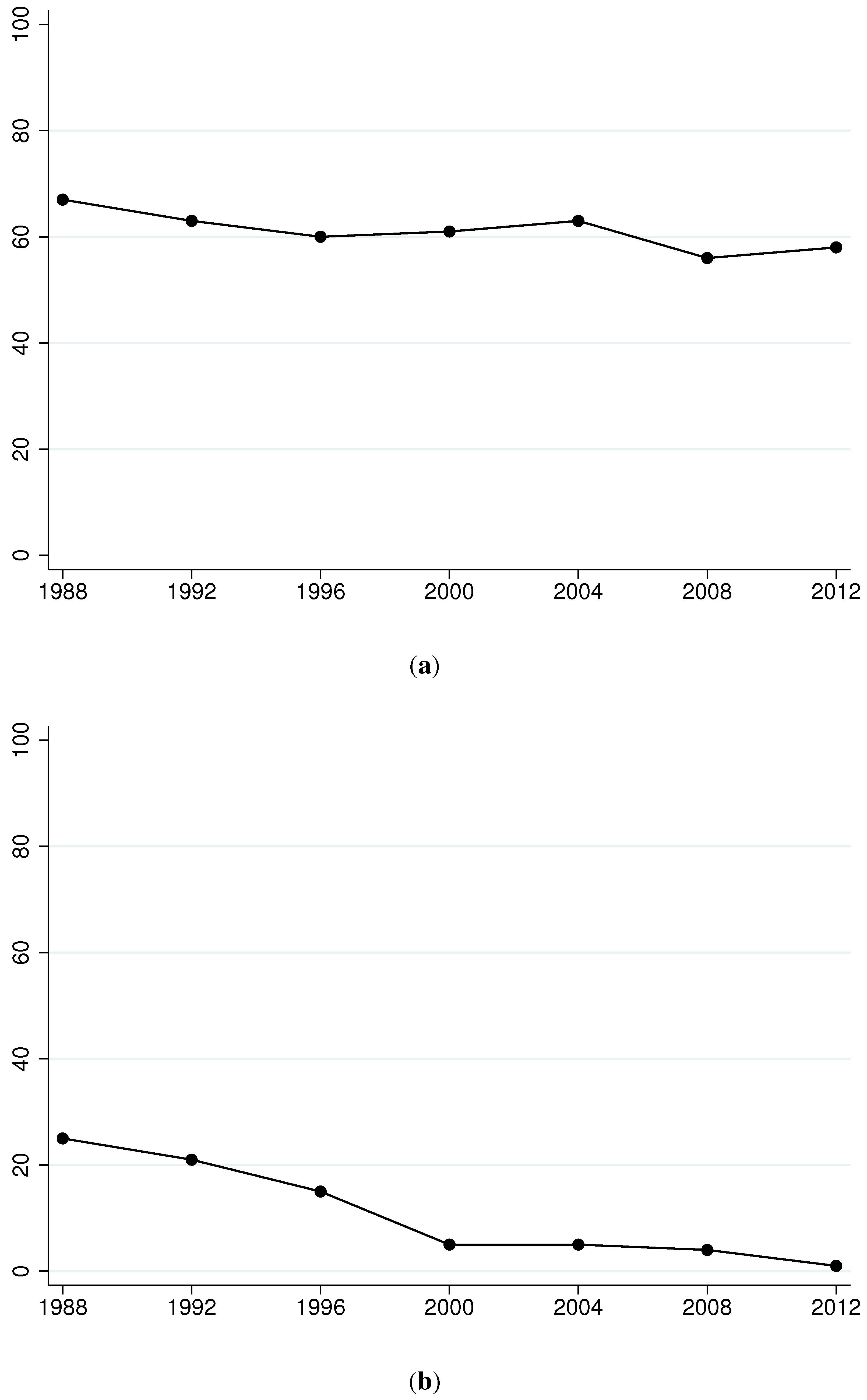
In the past seven Olympiads, between 56 and 66 percent of participating countries have not won any medals. To provide a more detailed description Table 2 shows frequency distributions by year. The numbers highlight the heavy concentration among zero winners. The panel (a) of Figure 1 provides a graphical depiction of the proportion of zero winners over time. On the other hand, while most countries do not win any medals, recent Olympic competitions have seen a small number of countries capture a majority of all medals awarded. For example, during the 2012 games, ten countries (the United States, China, Great Britain, Russia, South Korea, Germany, France, Italy, Hungary and Australia) captured 55 percent of total medals.

Table 2. Frequency distribution of total awarded medals for seven Olympiads.

Number of Medals Won	1988	1992	1996	2000	2004	2008	2012
0	66.2 (98)	62.3 (99)	58.8 (110)	59.6 (112)	61.6 (117)	55.7 (108)	56.0 (108)
1–5	18.9 (28)	22.6 (36)	23.0 (43)	22.9 (43)	18.9 (36)	25.8 (50)	24.9 (48)
6–10	2.7 (4)	3.8 (6)	5.9 (11)	5.3 (10)	8.9 (17)	8.2 (16)	7.3 (14)
11–15	4.1 (6)	1.3 (2)	3.7 (7)	3.7 (7)	1.6 (3)	2.1 (4)	3.6 (7)
16–20	1.4 (2)	3.8 (6)	2.1 (4)	1.6 (3)	2.1 (4)	2.1 (4)	3.1 (6)
21–25	2.0 (3)	1.3 (2)	2.1 (4)	1.6 (3)	1.1 (2)	1.0 (2)	0.0 (0)
> 25	4.7 (7)	5.0 (8)	4.8 (9)	5.3 (10)	5.8 (11)	5.2 (10)	5.2 (10)

Notes: The numbers refer to percentage of countries in each size class. The number in parentheses refers to the number of countries.

Table 2. Frequency distribution of total awarded medals for seven Olympiads.

Number of Medals Won	1988	1992	1996	2000	2004	2008	2012
0	66.2 (98)	62.3 (99)	58.8 (110)	59.6 (112)	61.6 (117)	55.7 (108)	56.0 (108)
1–5	18.9 (28)	22.6 (36)	23.0 (43)	22.9 (43)	18.9 (36)	25.8 (50)	24.9 (48)
6–10	2.7 (4)	3.8 (6)	5.9 (11)	5.3 (10)	8.9 (17)	8.2 (16)	7.3 (14)
11–15	4.1 (6)	1.3 (2)	3.7 (7)	3.7 (7)	1.6 (3)	2.1 (4)	3.6 (7)
16–20	1.4 (2)	3.8 (6)	2.1 (4)	1.6 (3)	2.1 (4)	2.1 (4)	3.1 (6)
21–25	2.0 (3)	1.3 (2)	2.1 (4)	1.6 (3)	1.1 (2)	1.0 (2)	0.0 (0)
> 25	4.7 (7)	5.0 (8)	4.8 (9)	5.3 (10)	5.8 (11)	5.2 (10)	5.2 (10)

Notes: The numbers refer to percentage of countries in each size class. The number in parentheses refers to the number of countries.

Figure 1. Characteristics of Olympic winnings and participation. (a) Share of zero-medal winners; (b) Share of countries with no female participation; (c) Changes in the share of female athletes; (d) Female participation in 1988 and 2008.

Figure 1. Characteristics of Olympic winnings and participation. (a) Share of zero-medal winners; (b) Share of countries with no female participation; (c) Changes in the share of female athletes; (d) Female participation in 1988 and 2008.

The numbers suggest that medal winnings may be modeled as a two-stage process in which the first stage determines the conditional probability of winning one or more medals, and the second stage determines the number of medals conditional on winning at least one. Such a two-stage setup is motivated by evidence that, while sending athletes to compete is not, by itself, prohibitively expensive, the process of developing potential winners does appear to require significant financial resources [14,17].

As an indicator of persistence in performance at successive Olympiads, Table 3 reports the percent of countries in each year that win zero medals after also winning zero medals in the previous Olympiad. The table also provides the percent of countries that win more than 25 medals after also winning more than 25 in the previous Olympiad. We are also interested in why countries might deviate from previously persistent states. On one hand, countries might experience sudden success (or loss), perhaps due to the emergence of uniquely-talented athletes, only to return to previous states in subsequent Olympiads. Alternatively, countries might experience sudden success (or loss), which then diverts the country to a more permanent path of success or failure.

Table 3. Persistent winners and non-winners.

1988	1992	1996	2000	2004	2008	2012
Persistent zero winners
–	90%	88%	88%	91%	85%	89%
Persistent > 25 winners
–	75%	64%	89%	91%	82%	90%

Table 3. Persistent winners and non-winners.

1988	1992	1996	2000	2004	2008	2012
Persistent zero winners
–	90%	88%	88%	91%	85%	89%
Persistent > 25 winners
–	75%	64%	89%	91%	82%	90%

The Beveridge and Nelson [18] decomposition of a time series into permanent and transitory components is well-established but has not been extended to our discrete non-linear panel setup. However, Table 4 provides informal evidence based on observed transitions in the estimation sample. Taking the first entry as an example, 88 percent of countries that failed to win any medal at an Olympiad also failed to win any at the subsequent Olympiad. On the other hand, 12 percent of zero winners proceeded to win 1−5 medals at the subsequent Olympiad. None proceeded to win more than 6 medals. At the other extreme, among countries that won more than 25 medals, 88 percent also won more than 25 at the subsequent Olympiad, with the remaining 12 percent winning 16−25 medals. The largest numbers in the table appear along the main diagonal, with relatively small values in the off-diagonals. This provides informal evidence that deviations in persistence tend to be relatively transitory.

Table 4. Transitions between categories of winners.

Observed Frequencies of Medal Winnings
		Medals Won at Subsequent Olympiad
		0	1–5	6–15	16–25	>25
Medals Won at Previous Olympiad	0	0.88	0.12	0.00	0.00	0.00
	1–5	0.26	0.60	0.14	0.00	0.00
	6–15	0.01	0.26	0.58	0.13	0.02
	16–25	0.00	0.03	0.28	0.51	0.18
	>25	0.00	0.00	0.00	0.12	0.88

Table 4. Transitions between categories of winners.

Observed Frequencies of Medal Winnings
		Medals Won at Subsequent Olympiad
		0	1–5	6–15	16–25	>25
Medals Won at Previous Olympiad	0	0.88	0.12	0.00	0.00	0.00
	1–5	0.26	0.60	0.14	0.00	0.00
	6–15	0.01	0.26	0.58	0.13	0.02
	16–25	0.00	0.03	0.28	0.51	0.18
	>25	0.00	0.00	0.00	0.12	0.88

2.2. Female Participation

In 1988 nearly one-quarter of participating countries had no female participation, whereas in 2012, only two countries (Barbados and Nauru) sent all-male contingents. Table 5 shows the evolution of female participation over time. Although the number of female participants continues to increase, the majority of countries still send 0−5 females. At the other end of the distribution, 15−23 percent of countries send more than 25 females. The panel (b) of Figure 1 provides a graphical depiction of the proportion of countries that send zero females.

Table 5. Female participation in seven Olympiads.

Number of Females	1988	1992	1996	2000	2004	2008	2012
0	24.3 (36)	21.4 (34)	15.0 (28)	5.3 (10)	4.7 (9)	4.7 (9)	1.0 (2)
1–5	45.9 (68)	46.5 (74)	49.2 (92)	51.6 (97)	54.2 (103)	53.1 (103)	55.7 (113)
6–10	7.4 (11)	8.8 (14)	9.6 (18)	11.2 (21)	8.9 (17)	7.2 (14)	7.4 (15)
11–15	2.0 (3)	2.5 (4)	3.7 (7)	5.3 (10)	4.2 (8)	6.2 (12)	4.4 (9)
16–20	2.7 (4)	0.6 (1)	4.3 (8)	3.7 (7)	7.9 (15)	4.6 (9)	4.9 (10)
21–25	2.7 (4)	3.1 (5)	1.6 (3)	2.7 (5)	3.2 (6)	3.6 (7)	3.4 (7)
>25	15.5 (23)	17.0 (27)	16.6 (31)	20.2 (38)	16.8 (32)	20.6 (40)	23.2 (47)

Notes: The numbers refer to percentage of countries in each size class. The number in parentheses refers to the number of countries.

Table 5. Female participation in seven Olympiads.

Number of Females	1988	1992	1996	2000	2004	2008	2012
0	24.3 (36)	21.4 (34)	15.0 (28)	5.3 (10)	4.7 (9)	4.7 (9)	1.0 (2)
1–5	45.9 (68)	46.5 (74)	49.2 (92)	51.6 (97)	54.2 (103)	53.1 (103)	55.7 (113)
6–10	7.4 (11)	8.8 (14)	9.6 (18)	11.2 (21)	8.9 (17)	7.2 (14)	7.4 (15)
11–15	2.0 (3)	2.5 (4)	3.7 (7)	5.3 (10)	4.2 (8)	6.2 (12)	4.4 (9)
16–20	2.7 (4)	0.6 (1)	4.3 (8)	3.7 (7)	7.9 (15)	4.6 (9)	4.9 (10)
21–25	2.7 (4)	3.1 (5)	1.6 (3)	2.7 (5)	3.2 (6)	3.6 (7)	3.4 (7)
>25	15.5 (23)	17.0 (27)	16.6 (31)	20.2 (38)	16.8 (32)	20.6 (40)	23.2 (47)

Notes: The numbers refer to percentage of countries in each size class. The number in parentheses refers to the number of countries.

The skewed distribution of female participants reflects, in part, the skewed distribution of the number of overall participants. Therefore, we calculate the proportion of each country’s contingent that consists of females. The panel (c) of Figure 1 shows female proportions over time. Aggregate female participation rose from 17 percent in 1988 to 36 percent in 2000 to more than 40 percent in 2012. Recent Olympiads also have witnessed a marked increase in countries that send majority female contingents. In 1988 only 4 countries sent more females than male competitors, but 34 countries did so in 2012. Among countries that were awarded at least one medal, only two countries had higher female than male participation in 1988, and this number rose to 14 by 2012. The panel (d) of Figure 1 shows a quantile plot that attempts to summarize the considerable intra-country variation in female contingent shares for the first and last Olympiads in our data. The graph confirms the increase in female participation over time, including a decrease in the percentage of countries that send zero females. The figure also indicates that, at the 2012 games, approximately half of participating countries fielded contingents that consisted of at least 40 percent females. At the 1988 games, in contrast, fewer than 10 percent of participating countries fielded squads of more than 40 percent females.

2.3. Other Variables

Table 6 presents definitions and sample means for other variables used in our empirical analysis. PCGDP, population, and athlete shares are scaled and logged, due to their highly skewed shapes. Female share, despite also being skewed, is not logged due to its high probability mass at 0. Another variable indicates the 11 percent of participating countries that declare themselves to be Islamic states (meaning Muslim counties that expressly have no distinction between civil/government and religious affairs) and/or have Islam as the officially-declared state religion. Traditionally, in the Islamic culture female participation in certain sporting activities has been discouraged. Of course, this implies that the Islamic dummy, to some extent, is collinear with female athlete share, but we include both Islamic status and female share, because we also must account for possible low female participation among the approximately 89 percent of our data points that are not Islamic.

Table 6. Sample means of explanatory variables based on 1313 country/Olympiads.

Variable	Definition	Mean	Between Country Standard. Dev.	Within Country Standard. Dev.
Number of medals	Number of medals won	4.59	16.62	3.22
Athlete share	$ln\left(\frac{\text{country’s}\text{athletes}}{\text{total}\text{athletes}}\right)$	−6.38	1.49	0.40
Female share	$\frac{\text{country’s}\text{females}}{\text{total}\text{athletes}}$	0.31	0.12	0.15
Per capita GDP	$ln\left(\frac{\text{GDP}}{\text{10,000}*\text{population}}\right)$	−1.15	1.61	0.61
Population	$ln\left(\frac{\text{population}}{\text{10,000,000}}\right)$	−0.84	2.33	0.16
Islamic	=1 if Islamic, 0 otherwise	0.11	0.31	0
Host	=1 if host, 0 otherwise	0.01	0.03	0.07

Table 6. Sample means of explanatory variables based on 1313 country/Olympiads.

Variable	Definition	Mean	Between Country Standard. Dev.	Within Country Standard. Dev.
Number of medals	Number of medals won	4.59	16.62	3.22
Athlete share	$ln\left(\frac{\text{country’s}\text{athletes}}{\text{total}\text{athletes}}\right)$	−6.38	1.49	0.40
Female share	$\frac{\text{country’s}\text{females}}{\text{total}\text{athletes}}$	0.31	0.12	0.15
Per capita GDP	$ln\left(\frac{\text{GDP}}{\text{10,000}*\text{population}}\right)$	−1.15	1.61	0.61
Population	$ln\left(\frac{\text{population}}{\text{10,000,000}}\right)$	−0.84	2.33	0.16
Islamic	=1 if Islamic, 0 otherwise	0.11	0.31	0
Host	=1 if host, 0 otherwise	0.01	0.03	0.07

Finally, we include a variable indicating whether the country served as the host for the games. Stefani [19] identifies three main home team effects in team sports: “physiological, where the home team has traveled far less and is less fatigued; psychological, due to crowd support and territoriality pride; and tactical, in that the home team is more familiar with the playing conditions.” Stefani compares host nation medal winnings with those of four years earlier across 12 Olympiads since 1956 and estimates an average increase of 13 medals due to host status. Interestingly, the average decrease following the host status is reported to be 7 medals, indicating that some of the momentum from earlier success persists.

One specific advantage comes from the host country being able to field a relatively large number of competing athletes. Among the seven host countries in our sample, Table 7 illustrates that each country substantially boosted the size of its contingent during its host year, only to reduce the size at the subsequent Olympiad. Anticipating a key finding from our econometric model, this makes host status a noisy predictor of Olympic success, because although contingent sizes correlate with more medals, host countries, perhaps for public relation reasons, appear to field many athletes with little hope of winning. (As discussed below, this is especially true for Greece in 2000, which more than tripled the size of its contingent during its host year.)

Table 7. Number of athletes for host countries.

	Olympiad before Hosting	Olympiad of Hosting	Olympiad after Hosting
South Korea	−	401	226
Spain	229	422	289
USA	545	646	586
Australia	417	617	470
Greece	140	426	152
China	383	600	386
Great Britain	304	559	−

Table 7. Number of athletes for host countries.

	Olympiad before Hosting	Olympiad of Hosting	Olympiad after Hosting
South Korea	−	401	226
Spain	229	422	289
USA	545	646	586
Australia	417	617	470
Greece	140	426	152
China	383	600	386
Great Britain	304	559	−

Table 6 also shows within- and between-country standard deviations. The two variables that characterize a country’s athletic contingent (athlete share and female share) show little within-country variation. This means that there is continuity and persistence in these factors at the country level, but there is substantial between-country variation which makes potential identification of the role of these factors possible. Our socioeconomic measures (PCGDP, population, and Islamic culture) also display a similar feature.

3. Selection Model

This section develops a selection model to account for the large number of countries that win zero medals. We follow Bernard and Busse [7] in modeling the share of medals awarded to country i at time t, denoted $s_{it},$ $0\le s_{it}<1.$ This choice offers three advantages. First, it provides an intuitive interpretation as the average probability of winning a medal. Second, in contrast to total medals, medal shares indirectly account for interdependence across countries, in that one country’s victory necessarily implies another’s defeat. Third, it controls for nonstationarity in medal winnings due to the changing number of sports, as well as changing number of events within each sport, at successive Olympiads.

Modeling medal shares using simple linear regression methods is problematic, because it neglects the salient difficulty inherent in modeling Olympic performance: The majority of countries participating in an Olympiad fail to win any medal. Statistically, this implies that the distribution of variable $s_{it}$ shows large mass at zero, which is inconsistent with normality. This violation of normality also precludes usage of the standard Tobit approach.

As a departure, our selection setup treats the process of fielding winners and the subsequent level of success as two separate, but related, statistical processes. The model is a version of the so-called two-part model (TPM), extended to allow for correlation between random components of the two equations. Let $m_{it}$ equal 1 if country i won any medal in Olympiad t, and 0 otherwise. Let $m_{it}^{*}$ denote a latent variable such that

$$m_{it}=\left\{\begin{array}{c}1\text{if}{m}_{it}^{*}>0\\ 0\text{if}{m}_{it}^{*}\le 0\end{array}\right.$$

(1)

and the resulting outcome equation for shares is

$$s_{it}=\left\{\begin{array}{c}{s}_{it}^{*}\text{if}{m}_{it}^{*}>0\\ -\text{if}{m}_{it}^{*}\le 0\end{array}\right.$$

(2)

where $s_{it}^{*}$ is a latent variable. A variant of the standard model with additive errors is

$$\begin{array}{ccc}\hfill m_{it}^{*}& =& {\mathbf{z}}_{it}^{\prime }\gamma +{\xi }_{it}\hfill \end{array}$$

$$\begin{array}{ccc}\hfill g\left(s_{it}^{*}\right)& =& {\mathbf{x}}_{it}^{\prime }\beta +c_{it}\hfill \end{array}$$

(3)

where ${\xi }_{it}$ and $c_{it}$ represent error terms. We refer to the first equation as the “selection” equation, and the second as the “outcome” equation. Although we discuss estimates from the selection equation below, our primary interest lies in the outcome equation, which captures the level of success conditional on having won any medals. The vectors ${\mathbf{z}}_{it}$ and ${\mathbf{x}}_{it}$ represent explanatory variables, discussed in more detail below. The vectors need not differ for identification purposes, although in this paper, we include several “exclusion restrictions” in ${\mathbf{z}}_{it}$ that do not appear in ${\mathbf{x}}_{it}$. The vectors γ and β denote estimable coefficients.

Because in this paper we model medal shares, we wish to maintain the restriction $s_{it}\in$$[0,1)$ for predictive purposes. To impose this restriction we model the transformation $g\left(s_{it}\right)$, defined as $ln[s_{it}/(1-s_{it})]$, based on the standard logit transformation. A disadvantage of this step is that retransformation will be necessary should the focus of inquiry shift to the number of medals, as it might if we wish to compare the actual winning total with that conditionally fitted by the model.

To accommodate unobserved country-specific heterogeneity, we specify the error terms ${\xi }_{it}$ and $c_{it}$ using two different approaches. In the first, we specify

$$\begin{array}{ccc}\hfill {\xi }_{it}& =& {\eta }_{1i}+{\epsilon }_{1,it}\hfill \\ \hfill c_{it}& =& {\eta }_{2i}+{\epsilon }_{2,it}\hfill \end{array}$$

(4)

where ${\epsilon }_{1,it}$ and ${\epsilon }_{2,it}$ follow a standardized bivariate normal distribution with contemporaneous covariance ${\sigma }_{12}$, and the time invariant terms, ${\eta }_{1i}$ and ${\eta }_{2i}$, are treated as random effects. The random effects approach is appropriate if country-specific heterogeneity does not vary significantly over time, and if heterogeneity does not correlate with observed predictors included in the model. 1

However, to relax the random effects assumptions, we also propose an alternative formulation,

$$\begin{array}{ccc}\hfill {\xi }_{it}& =& \rho m_{i,t-1}+{\epsilon }_{1,it}\hfill \\ \hfill c_{it}& =& {\mathbf{S}}_{i,t-1}^{\prime }\delta +{\epsilon }_{2,it}\hfill \end{array}$$

(5)

where ${\epsilon }_{1,it}$ and ${\epsilon }_{2,it}$ follow a standardized bivariate normal distribution as before, and where $m_{i,t-1}$ indicates whether the country won a medal at the previous Olympiad, and ${\mathbf{S}}_{i,t-1}$ denotes a vector of categorical variables that measures success at the previous Olympiad,

$$\begin{array}{c}{D}_{1,it}=1[.75<s_{i,t-1}\le .90]\hfill \\ D_{2,it}=1[.90<s_{i,t-1}\le .95]\hfill \\ D_{3,it}=1[.95<s_{i,t-1}\le .99]\hfill \\ D_{4,it}=1[.99<s_{i,t-1}]\hfill \end{array}$$

(6)

Falling below the 75th percentile (which occurs at approximately 0 medals) represents the reference group. The motivation for this dynamic specification arises from possible improvements that may come if we can capture the role of sports culture mentioned earlier. Under the assumption that sports culture persists over time, a lagged measure of Olympic success is a reasonable proxy variable for sports culture. However, alternative interpretations for including this variable can also be offered; for example, it may capture the effects of momentum due to past success.

Estimation of the selection model follows a two-step approach. We first estimate the probability of winning any medal, using either the random effects or the dynamic specification,

$$\begin{array}{cc}\mathrm{random} \mathrm{effects}:\hfill & \mathrm{Pr}(m_{it}=1|{\mathbf{z}}_{it},{\eta }_{1i})=\text{Φ}({\mathbf{z}}_{it}^{\prime }\gamma +{\eta }_{1i})\hfill \\ \mathrm{dynamic}:\hfill & \mathrm{Pr}(m_{it}=1|{\mathbf{z}}_{it},m_{i,t-1})=\text{Φ}({\mathbf{z}}_{it}^{\prime }\gamma +\rho m_{i,t-1})\hfill \end{array}$$

(7)

We assume that in the random effects equation, ${\mathbf{z}}_{it}$ are strictly exogenous, and ${\eta }_{1i}$ are independent from $({\epsilon }_{1,it},{\epsilon }_{2,it})$; in the dynamic equation, ${\mathbf{z}}_{it}$ are strictly exogenous and $m_{i,t-1}$ is weakly exogenous and uncorrelated with $({\epsilon }_{1,it},{\epsilon }_{2,it})$. By definition $D_{j,it}$$(j=1,..,4)$ are group-specific variables, the group being the set of countries that fall in a particular interquartile range. Therefore, we should expect a low correlation between them and country-specific shocks $({\epsilon }_{1,it},{\epsilon }_{2,it})$. We further assume that ${\epsilon }_{1,it}$ and ${\epsilon }_{2,it}$ are serially independent. These assumptions are similar to those used by Semykina and Wooldridge [21] in their model which handles both selection and endogeneity.

Using estimates obtained from the first-stage selection equation, we calculate inverse Mill’s ratio terms, $\lambda \left({\mathbf{z}}_{it}^{\prime }\widehat{\gamma }\right)$ for the random effects model, and $\lambda ({\mathbf{z}}_{it}^{\prime }\widehat{\gamma }+\widehat{\rho }{m}_{i,t-1})$ for the dynamic model, where $\lambda (·)=\varphi (·)/\Phi \left(·\right)$. In the second step, the inverse Mill’s ratio is then included in the outcome equation,

$$\begin{array}{cc}\mathrm{random} \mathrm{effects}:\hfill & E[g(s_{it}^{*})|{\mathbf{x}}_{it},{\mathbf{z}}_{it},{\eta }_{2i},m_{it}=1]={\mathbf{x}}_{it}^{\prime }\beta +{\sigma }_{12}\lambda (·)+{\eta }_{2i}\hfill \\ \mathrm{dynamic}:\hfill & E[g(s_{it}^{*})|{\mathbf{x}}_{it},{\mathbf{z}}_{it},{\mathbf{S}}_{i,t-1},m_{it}=1]={\mathbf{x}}_{it}^{\prime }\beta +{\sigma }_{12}\lambda (·)+{\mathbf{S}}_{i,t-1}^{\prime }\mathbf{\delta }\hfill \end{array}$$

(8)

where ${\sigma }_{12}$ denotes the covariance of $({\epsilon }_1,{\epsilon }_2)$. Similar to the selection equations, in the first equation ${\mathbf{x}}_{it}$ and ${\eta }_{2i}$ are independent from ${\epsilon }_{2,it}$, and in the second equation ${\mathbf{x}}_{it}$ and $S_{i,t-1}$ are independent from ${\epsilon }_{2,it}$.

4. Structural Treatment of Athletic Participation

An argument for treating the country’s level of participation—a key explanatory variable in the outcome equation—as exogenous follows from the recursive process involved in country representation. That is, a country’s measured participation level is determined prior to the Olympiad and does not capture discretionary variations after the games have started. However, participation is conditional on reaching in pre-Olympic trials and competitions the Olympic standard set by appropriate sports-specific administrative bodies. Potentially countries can (and do) influence this outcome by providing resources and opportunities for its athletes. In many cases such efforts are concentrated in events and on athletes where a country expects to or wants to excel. These factors are expected to be highly correlated with observable variables like country’s PCGDP and population size, and also with unmeasured variables like its sports culture, which is absorbed in the equation error. Hence there is a case for treating this variable as endogenous. Therefore, this section takes the selection model developed in the previous section and appends to it a structural framework describing a country’s level of participation. 2

Let Y denote a measure of Olympic success, and let ${\mathbf{x}}_{it}$ denote a vector of observable time-varying shift factors. Then medals are “produced” according to an aggregate relationship such as

$$Y_{it}=F\left({\mathbf{x}}_{it},{\text{participation}}_{it},c_{it}\right)$$

with the arguments of $F\left(·\right)$ interpreted as “inputs” with positive and diminishing marginal products. 3

The variable participation${}_{it}$ refers to the size and composition of the country’s athletic contingent. Our model views participation as being “produced” by the country’s resources, specifically PCGDP and population size, which, themselves, might proxy for access to training and facilities and the pool of sporting talent from which competitors are drawn,

$${\text{participation}}_{it}=H\left({\text{PCGDP}}_{it},{\text{population}}_{it},c_{it}\right)$$

Viewing the athletic contingent as “produced” emphasizes the importance of resources at the country level, a notion that was historically relevant. However, elite athletes now operate in a more “open” international setting in which they can choose to live, train, and practice in a foreign country, and yet also represent a different country in an international competition. Such international arbitrage of sporting talent is amply evident in soccer, tennis, and many field and track events. Its existence occasionally explains how a country might achieve a better performance than predicted on the basis of country-specific factors alone.

Such international arbitrage is one example of what we label “sports culture,” which presumablely affects a country’s participation as well as its subsequent success. While a somewhat amorphous concept, sports culture might reflect national characteristics, such as the breadth and intensity of national participation in the competitive Olympic type events. The development of such a culture may depend on a country’s sporting history, access to organization and training facilities at elite sports institutes, availability of financial resources, incentives for participation, and the size and depth of the pool of available athletes. In addition, sports culture might reflect persistent participation and/or success in certain athletic categories (see Manners’ [24] narrative account of “Kenya’s running tribe”).

Sports culture, however defined and whatever its origin, affects both participation and medal winnings. We denote it as $c_{it}$ in the two production functions listed above. As discussed above, we propose two different approaches for introducing $c_{it}$ into the empirical model. The first assumes that the latent variable is a time-invariant, country-specific factor that does not correlate with other regressors in the model. Thus, $c_i$ is treated as a random effect. The second approach recognizes that the latent term can, and likely does, vary over time depending on past performance according to $c_{it}=g\left(Y_{i,t-1}\right)$ where $g\left(·\right)$ is some function.

To deal with the endogeneity of athlete share in the second-stage equations, we estimate a version of a model proposed by Blundell et al. [25] and expanded by Das et al. [26]. The essential idea is that, in addition to including $\lambda (·)$ to account for selection, the outcome equation also includes a control function obtained from a first-stage reduced form simple linear regression of athlete share on ${\mathbf{z}}_{it}$. Specifically, we regress athlete share on ${\mathbf{z}}_{it}$, and then, in what follows, predicted athlete shares from that regression are denoted $K\left({\mathbf{z}}_{it}\right)$. 4

We cannot use this same approach in the selection part of the model (i.e., Equation (7)), because all ${\mathbf{z}}_{it}$ variables appear in that first stage. However, assuming that athlete share is a linear function of regressors, we essentially “substitute” athlete share out of the equation, leaving all of the remaining variables ${\mathbf{z}}_{it}$ that influence athlete share. That is, to address potential endogeneity of athlete we simply remove it from the first stage, giving the first stage a reduce form interpretation.

5. Explanatory Variables and Estimation

Bringing together the two previous sections, we address selection and endogeneity of athlete shares by estimating the outcome equations as

$$\begin{array}{cc}\mathrm{random} \mathrm{effects}:\hfill & E[g(s_{it}^{*})|{\mathbf{x}}_{it},{\mathbf{z}}_{it},{\eta }_{2i},m_{it}=1]={\mathbf{x}}_{it}^{\prime }\beta +{\sigma }_{12}\lambda (·)+\delta K({\mathbf{z}}_{it})+{\eta }_{2i}\hfill \\ \mathrm{dynamic}:\hfill & E[g(s_{it}^{*})|{\mathbf{x}}_{it},{\mathbf{z}}_{it},{\mathbf{S}}_{i,t-1},m_{it}=1]={\mathbf{x}}_{it}^{\prime }\beta +{\sigma }_{12}\lambda (·)+\delta K({\mathbf{z}}_{it})+{\mathbf{S}}_{i,t-1}^{\prime }\mathbf{\delta }\hfill \end{array}$$

(9)

where ${\sigma }_{12}$ and δ are to be estimated along with β. (Note: In later discussion we absorb $\lambda (·)$ and $K\left({\mathbf{z}}_{it}\right)$ into ${\mathbf{x}}_{it}$, and we absorb ${\sigma }_{12}$ and δ into β for notational brevity.)

Variables included in ${\mathbf{x}}_{it}$ capture details of the country’s athletic contingent: (1) athlete share defined as each country’s number of athletes expressed as a proportion of all athletes; (2) the female proportion of each country’s contingent; and (3) an indicator of host status. 5

In addition to those variables listed in the previous paragraph, the vector ${\mathbf{z}}_{it}$ includes three variables that do not appear in ${\mathbf{x}}_{it}$: (1) PCGDP; (2) population; and (3) Islamic. (Note, ${\mathbf{z}}_{it}$ does not include the host status indicator, as it perfectly generates the probability of winning any medal.) Note that, consistent with our structural interpretation of the model, these three variables affect medal winnings only through their influence on producing the country’s athletic contingent. Consequently, PCGDP, population, and Islamic serve as exclusion restrictions in the selection model and control function setup.

The random effects models are estimated using Stata’s xtprobit command for the selection equation, and using xtreg for the shares equation. The dynamic specifications are estimated using regular probit for the selection equation, and using regular OLS for the shares equation. The main additional complication of this approach is the computation of the asymptotic variance due to the use of generated regressor; see [27] for details. We are unaware of the precise modification required for the computing the asymptotic variance matrix of the second stage estimates, but the literature offers many examples in which this is done using the bootstrap method. Standard errors reported below adjust for clustering at the country level.

As previously noted, our approach to handling both selection and endogeneity has similarities with the model proposed by Semykina and Wooldridge [21]. Specifically, the Semykina and Wooldridge model requires strict exogeneity of the covariates in the selection equation (${\mathbf{z}}_{it}$), the selection process ($m_{it}$), and the unobserved country-specific effect (${\eta }_{2i}$). That is, in period t, the error term in the outcome equation (${\epsilon }_{2,it}$) must not correlate with past, present, or future values of $\left({\mathbf{z}}_{it},m_{it},{\eta }_{2i}\right)$. Our model also requires that the selection process ($m_{it}$) does not correlate with the country-specific effect (${\eta }_{2i}$); the correlation is expected to be weak as the country-specific effect is time-invariant and $m_{it}$ varies over time and country.

6. Results

This section first discusses estimates from the selection equation of the probability of winning any medal. We then proceed to discuss the level of Olympic success, conditional on having won any medal. Finally, we present fitted medal winnings from these models.

6.1. Selection: The Probability of Winning Any Medal

Table 8 presents estimates of models in which athlete share is treated as exogenous (first two columns) and then as endogenously determined, as discussed above, by removing it from the equation, which assumes that athlete share is a linear function of the other explanatory variables. The table also presents average marginal effects, although those magnitudes are difficult to interpret due to the scaling of the explanatory variables.

The most important explanatory variables, both in terms of magnitude and significance, are those that describe a country’s participation in the games. Not surprisingly, higher athlete shares correlate with larger probabilities of winning a medal. Larger female shares also appear to associate with larger probabilities in the static model that treats athlete share as exogenous, but female shares lose statistical significance in the other specifications. As for socioeconomic measures, population size, PCGDP, and Islamic are only marginally significant when athlete share is treated as exogenous, but those three variables are much larger in magnitude, and more precisely estimated, when athlete share is treated as endogenous.

The dynamic specifications highlight the high degree of persistence in Olympic performance, in that past winning strongly correlates with present winning. Coefficients of all other explanatory variables shrink in magnitude in the dynamic specifications, which may be expected as those variables, themselves, show high degrees of persistence.

Table 8. Probit estimates of the probability of winning any medal (average marginal effects in brackets).

	Static Model		Dynamic Model		Static Model		Dynamic Model
	(1)		(2)		(3)		(4)
	Coeff.	St. Err.	Coeff.	St. Err.	Coeff.	St. Err	Coeff.	St. Err
Athlete share	1.134 ${}^{*}$	0.091	0.886 ${}^{*}$	0.084	•	•	•	•
	[0.16]		[0.13]
Female share	0.923 ${}^{*}$	0.382	0.280	0.362	−0.395	0.398	−0.559 ${}^{†}$	0.319
	[0.13]		[0.04]		[−0.08]		[−0.10]
Per capita GDP	0.129 ${}^{*}$	0.058	0.066	0.049	0.520 ${}^{*}$	0.065	0.323 ${}^{*}$	0.038
	[0.02]		[0.01]		[0.10]		[0.06]
Population	0.158 ${}^{*}$	0.057	0.070	0.044	0.761 ${}^{*}$	0.073	0.342 ${}^{*}$	0.036
	[0.02]		[0.01]		[0.15]		[0.06]
Islamic	−0.161	0.254	−0.005	0.191	−1.434 ${}^{*}$	0.395	−0.499 ${}^{*}$	0.170
	[−0.02]		[<−0.01]		[−0.27]		[−0.09]
Constant	6.815 ${}^{*}$	0.523	5.030 ${}^{*}$	0.520	0.977 ${}^{*}$	0.225	−0.133	0.157
Any medal${}_{t-1}$	−	−	0.865 ${}^{*}$	0.138	−	−	1.611 ${}^{*}$	0.115
			[0.12]				[0.29]
Random effects?	Yes		No		Yes		No
Random effect variance	0.636		−		1.359		−
Log likelihood	−366.57		−286.65		−443.91		−353.32
Sample size	1313		1098		1,313		1,098

Note: Athlete share is treated as exogenous in the first two columns; • Athlete share assumed endogenously determined as a linear function of included exogenous variables. *: p < 0.05; † : p < 0.10

Table 8. Probit estimates of the probability of winning any medal (average marginal effects in brackets).

	Static Model		Dynamic Model		Static Model		Dynamic Model
	(1)		(2)		(3)		(4)
	Coeff.	St. Err.	Coeff.	St. Err.	Coeff.	St. Err	Coeff.	St. Err
Athlete share	1.134 ${}^{*}$	0.091	0.886 ${}^{*}$	0.084	•	•	•	•
	[0.16]		[0.13]
Female share	0.923 ${}^{*}$	0.382	0.280	0.362	−0.395	0.398	−0.559 ${}^{†}$	0.319
	[0.13]		[0.04]		[−0.08]		[−0.10]
Per capita GDP	0.129 ${}^{*}$	0.058	0.066	0.049	0.520 ${}^{*}$	0.065	0.323 ${}^{*}$	0.038
	[0.02]		[0.01]		[0.10]		[0.06]
Population	0.158 ${}^{*}$	0.057	0.070	0.044	0.761 ${}^{*}$	0.073	0.342 ${}^{*}$	0.036
	[0.02]		[0.01]		[0.15]		[0.06]
Islamic	−0.161	0.254	−0.005	0.191	−1.434 ${}^{*}$	0.395	−0.499 ${}^{*}$	0.170
	[−0.02]		[<−0.01]		[−0.27]		[−0.09]
Constant	6.815 ${}^{*}$	0.523	5.030 ${}^{*}$	0.520	0.977 ${}^{*}$	0.225	−0.133	0.157
Any medal${}_{t-1}$	−	−	0.865 ${}^{*}$	0.138	−	−	1.611 ${}^{*}$	0.115
			[0.12]				[0.29]
Random effects?	Yes		No		Yes		No
Random effect variance	0.636		−		1.359		−
Log likelihood	−366.57		−286.65		−443.91		−353.32
Sample size	1313		1098		1,313		1,098

Note: Athlete share is treated as exogenous in the first two columns; • Athlete share assumed endogenously determined as a linear function of included exogenous variables. *: p < 0.05; † : p < 0.10

To assess the fit of the selection equation, Table 9 shows fitted values (“predictions”) of winning at least one medal based on the “dynamic/endogenous” model (last column in Table 8). We use outcome classification based on fitted probability cut-off of $0.5$ as a criterion for evaluating model fit. As shown in the table, the model correctly predicts 88 percent of outcomes, which attests to the fit of the selection part of the model. The most common misses, which total 79, correspond to incorrect predictions of zero medals, typically for “small” countries. Table 10 lists those 79 incorrect classifications. The fact that some countries, such as Algeria and Mongolia, appear multiple times points to persistent features of Olympic performance that even our dynamic specification does not fully capture. Figure 2 shows kernel density estimates of predicted probabilities for the misses from the selection model. These plots hint at a departure from unimodality, which, in turn, suggests that the modeling deficiency may be associated with different reasons for different countries.

Table 9. Fit of probit model 4.

			Predicted
			>0 Medals	0 Medals
Actual	>0 medals		360	79
	0 medals		54	605

Table 9. Fit of probit model 4.

			Predicted
			>0 Medals	0 Medals
Actual	>0 medals		360	79
	0 medals		54	605

Table 10. Countries that won at least one, but model predicted zero medals.

Country	Year	Country	Year	Country	Year
Afghanistan	2008	Iceland	2000	Qatar	2000
Algeria	1992	Iceland	2008	Qatar	2012
Algeria	2008	Ireland	1992	Saudi Arabia	2000
Armenia	2008	Israel	1992	Saudi Arabia	2012
Bahamas	1992	Kuwait	2000	Singapore	2008
Bahrain	2008	Kuwait	2012	Sri Lanka	2000
Barbados	2000	Kyrgyz Republic	2000	Sudan	2008
Cameroon	2000	Kyrgyz Republic	2008	Suriname	1992
Chile	2000	Macedonia	2000	Syria	1996
Chinese Taipei	1992	Malaysia	1992	Syria	2004
Colombia	2000	Malaysia	2008	Tajikistan	2008
Costa Rica	1996	Mauritius	2008	Togo	2008
Cyprus	2012	Moldova	2008	Tonga	1996
Dominican Republic	2004	Mongolia	1992	Trinidad and Tobago	1996
Ecuador	1996	Mongolia	1996	Tunisia	1996
Ecuador	2008	Mongolia	2004	Tunisia	2008
Egypt	2004	Montenegro	2012	Uganda	1996
Eritrea	2004	Mozambique	1996	Uganda	2012
Estonia	2000	Nigeria	1992	United Arab Emirates	2004
Gabon	2012	Norway	2004	U.S. Virgin Islands	2008
Ghana	1992	Panama	2008	Uruguay	2000
Grenada	2012	Paraguay	2004	Venezuela	2004
Guatemala	2012	Portugal	1996	Vietnam	2000
Hong Kong	1996	Puerto Rico	1992	Vietnam	2008
Hong Kong	2004	Puerto Rico	2012	Zambia	1996
Hong Kong	2012	Qatar	1992	Zimbabwe	2004

Table 10. Countries that won at least one, but model predicted zero medals.

Country	Year	Country	Year	Country	Year
Afghanistan	2008	Iceland	2000	Qatar	2000
Algeria	1992	Iceland	2008	Qatar	2012
Algeria	2008	Ireland	1992	Saudi Arabia	2000
Armenia	2008	Israel	1992	Saudi Arabia	2012
Bahamas	1992	Kuwait	2000	Singapore	2008
Bahrain	2008	Kuwait	2012	Sri Lanka	2000
Barbados	2000	Kyrgyz Republic	2000	Sudan	2008
Cameroon	2000	Kyrgyz Republic	2008	Suriname	1992
Chile	2000	Macedonia	2000	Syria	1996
Chinese Taipei	1992	Malaysia	1992	Syria	2004
Colombia	2000	Malaysia	2008	Tajikistan	2008
Costa Rica	1996	Mauritius	2008	Togo	2008
Cyprus	2012	Moldova	2008	Tonga	1996
Dominican Republic	2004	Mongolia	1992	Trinidad and Tobago	1996
Ecuador	1996	Mongolia	1996	Tunisia	1996
Ecuador	2008	Mongolia	2004	Tunisia	2008
Egypt	2004	Montenegro	2012	Uganda	1996
Eritrea	2004	Mozambique	1996	Uganda	2012
Estonia	2000	Nigeria	1992	United Arab Emirates	2004
Gabon	2012	Norway	2004	U.S. Virgin Islands	2008
Ghana	1992	Panama	2008	Uruguay	2000
Grenada	2012	Paraguay	2004	Venezuela	2004
Guatemala	2012	Portugal	1996	Vietnam	2000
Hong Kong	1996	Puerto Rico	1992	Vietnam	2008
Hong Kong	2004	Puerto Rico	2012	Zambia	1996
Hong Kong	2012	Qatar	1992	Zimbabwe	2004

Figure 2. Kernel density plots of predictions from the selection equation.

Figure 2. Kernel density plots of predictions from the selection equation.

The selection equation also generates predictions of countries expected to win at least one medal at every Olympiad, and also countries expected to never win a medal at any Olympiad. Table 11 lists “always winners”; that is, the countries for which the predicted probability of winning exceeds 0.50 at all six Olympiads after 1988. Similarly, Table 12 lists “never winners”; that is, countries for which the predicted probability is less than 0.50 in all six years. Considering evidence of persistence in Olympic success, these tables offer suggestive evidence of the probability of success for those countries in future Olympiads. However, predictions that stand the highest threat of being wrong are due to the emergence of exceptionally talented athletes from a country that has previously been a nonperformer but, following success, goes on to develop a “tradition” of excellence in some particular group of events. (Olympic history is replete with examples of such events. For example, prior to Abebe Bikila’s storied victory in the marathon in 1960, Ethiopia had not won any Olympic medals, but since then has won 37 medals in middle and long distance running, and at every Olympiad in which it has participated.)

Table 11. Predicted always winners.

Argentina	France	South Korea
Australia	France	Morocco
Austria	Great Britain	Mexico
Belgium	Greece	Netherlands
Bulgaria	Hungary	New Zealand
Brazil	Indonesia	Poland
Canada	India	Romania
Switzerland	Iran	Sweden
China	Italy	Thailand
Denmark	Jamaica	Turkey
Spain	Japan	United States
Finland	Kenya

Table 11. Predicted always winners.

Argentina	France	South Korea
Australia	France	Morocco
Austria	Great Britain	Mexico
Belgium	Greece	Netherlands
Bulgaria	Hungary	New Zealand
Brazil	Indonesia	Poland
Canada	India	Romania
Switzerland	Iran	Sweden
China	Italy	Thailand
Denmark	Jamaica	Turkey
Spain	Japan	United States
Finland	Kenya

Table 12. Predicted never winners.

Angola	Dominica	Madagascar	St. Lucia
Albania	Eritrea	Maldives	Sao Tome and Principe
Antigua and Barbuda	Fiji	Marshall Islands	Suriname
Aruba	Micronesia	Mali	Swaziland
Burundi	Gabon	Malta	Seychelles
Benin	Gambia	Montenegro	Chad
Bermuda	Guinea-Bissau	Monaco	Turkmenistan
Burkina and Faso	Equatorial Guinea	Mauritania	Timor-Leste
Bangladesh	Grenada	Malawi	Tonga
Belize	Guatemala	Burma	Tuvalu
Bolivia	Guyana	Nauru	Tanzania
Bosnia Herzegovina	Honduras	Niger	St. Vincent and the Grenadines
Brunei	Haiti	Nicaragua	Vanuatu
Bhutan	Iraq	Netherlands Antilles	Samoa
British Virgin Islands	Jordan	Nepal	Yemen
Botswana	Kiribati	Oman	Congo
Central African Republic	St. Kitts and Nevis	Palau	American Samoa
Cote d’Ivoire	Laos	Papau New Guinea	Andorra
Cook Islands	Lebanon	Rwanda	Guinea
Comoros	Libya	Solomon Islands	Palestine
Cape Verde	Liberia	Sierra Leone	U.S. Virgin Islands
Cayman Islands	Liechtenstein	El Salvador	Cambodia
Cyprus	Lesotho	San Marino	Guam
Djibouti	Luxembourg	Somalia

Table 12. Predicted never winners.

Angola	Dominica	Madagascar	St. Lucia
Albania	Eritrea	Maldives	Sao Tome and Principe
Antigua and Barbuda	Fiji	Marshall Islands	Suriname
Aruba	Micronesia	Mali	Swaziland
Burundi	Gabon	Malta	Seychelles
Benin	Gambia	Montenegro	Chad
Bermuda	Guinea-Bissau	Monaco	Turkmenistan
Burkina and Faso	Equatorial Guinea	Mauritania	Timor-Leste
Bangladesh	Grenada	Malawi	Tonga
Belize	Guatemala	Burma	Tuvalu
Bolivia	Guyana	Nauru	Tanzania
Bosnia Herzegovina	Honduras	Niger	St. Vincent and the Grenadines
Brunei	Haiti	Nicaragua	Vanuatu
Bhutan	Iraq	Netherlands Antilles	Samoa
British Virgin Islands	Jordan	Nepal	Yemen
Botswana	Kiribati	Oman	Congo
Central African Republic	St. Kitts and Nevis	Palau	American Samoa
Cote d’Ivoire	Laos	Papau New Guinea	Andorra
Cook Islands	Lebanon	Rwanda	Guinea
Comoros	Libya	Solomon Islands	Palestine
Cape Verde	Liberia	Sierra Leone	U.S. Virgin Islands
Cayman Islands	Liechtenstein	El Salvador	Cambodia
Cyprus	Lesotho	San Marino	Guam
Djibouti	Luxembourg	Somalia

6.1.1. Why the Model May Provide an Inadequate Fit for Small Countries

We emphasize that an important limitation of our approach is that the above classifications are generated using only aggregate data and without any knowledge of the country strength in any particular sporting event. The aggregate model ignores the ongoing arbitrage in international movement of athletes. In a world in which elite athletes can train and compete almost exclusively in countries with excellent support while representing another country (that may have provided little actual support) at the Olympics, such predictive lapses based on a model like ours are inevitable. (Kirsty Coventry, a two-time Olympic swimming medalist who represented Zimbabwe in 2004 and 2008, is one example; French-born Boukpeti, a 2008 canoing medalist representing Togo, is another.) The Wall Street Journal (5 June 2012) reported estimates that “ ... foreign athletes from US universities may have won 60 medals in 2008—more than 6% of the total.” Data reported there show major-conference US schools with the highest ratio of foreign Olympians; this varies between 70% to 89% in 2008, with Auburn (89%) and Arizona State (87%) being at the top of the list.

Another limitation arises from geopolitical changes, most notably the dissolution of the former Soviet Union and the emergence of Central Asian republics, that give rise to new countries with short Olympic histories from which reliable extrapolation is not possible. In an important sense, therefore, misclassifications generated by our models provide an incentive to look into the stories behind the “unexpected” outcomes, as discussed below.

6.2. Outcome: Conditional Model of the Level of Success

Table 13 shows reduced form estimates from a simple first stage OLS regression of athlete share used to generate the control function. The most noteworthy result is that countries appear to use their resources, PCGDP and population size, to field competitors. The third exclusion restriction (Islamic) strongly negatively relates to athlete share. Host countries send more athletes, as reported in Section 2. Finally, successful medal winnings at previous Olympiads appear to correlate with increased participation at subsequent Olympiads, although the three coefficients for previous medal shares above the 90th percentile do not appear to statistically differ from each other. The implication is that increased success beyond the 90th percentile does not translate to ever-higher athlete shares.

Table 14 shows estimates of the outcome equation both with and without the control function for endogeneity included. The table provides cluster-robust standard errors. The first static specification in Table 14 accounts for selection (via inclusion of the Mills ratio) but treats athlete share as exogenous. In that specification, both athlete share and female share have robustly determined positive coefficients. Statistically significant selection bias is also indicated. When the past performance variables are added, they appear highly significant. Introducing past performance in the model, however, does reduce the role and significance of athlete share and female share. It is notable that in the dynamic version of the model there is no longer a statistically significant selection effect. That is, such sample selection is adequately “captured” by the introduction of the lagged performance indicators. This result is plausible but not highlighted in previous studies that have employed the static pooled regression framework and, moreover, not tested for the presence of selection bias.

Table 13. Regression of a county’s athlete share.

	Coeff.	St. Err.
Female share	−1.224 ${}^{*}$	0.123
Host	0.611 ${}^{*}$	0.294
Per capita GDP	0.306 ${}^{*}$	0.015
Population	0.329 ${}^{*}$	0.012
Islamic	−0.638 ${}^{*}$	0.073
medal share${}_{t-1}$ <75th pct	omitted
medal share${}_{t-1}$ 75–90th pct	1.181 ${}^{*}$	0.067
medal share${}_{t-1}$ 90–95th pct	1.985 ${}^{*}$	0.107
medal share${}_{t-1}$ 95–99th pct	2.062 ${}^{*}$	0.123
medal share${}_{t-1}$ ≥99th pct	1.924 ${}^{*}$	0.238
Constant	−5.730 ${}^{*}$	0.061
R-square	0.78

*: p < 0.05; †: p < 0.10.

Table 13. Regression of a county’s athlete share.

	Coeff.	St. Err.
Female share	−1.224 ${}^{*}$	0.123
Host	0.611 ${}^{*}$	0.294
Per capita GDP	0.306 ${}^{*}$	0.015
Population	0.329 ${}^{*}$	0.012
Islamic	−0.638 ${}^{*}$	0.073
medal share${}_{t-1}$ <75th pct	omitted
medal share${}_{t-1}$ 75–90th pct	1.181 ${}^{*}$	0.067
medal share${}_{t-1}$ 90–95th pct	1.985 ${}^{*}$	0.107
medal share${}_{t-1}$ 95–99th pct	2.062 ${}^{*}$	0.123
medal share${}_{t-1}$ ≥99th pct	1.924 ${}^{*}$	0.238
Constant	−5.730 ${}^{*}$	0.061
R-square	0.78

*: p < 0.05; †: p < 0.10.

The third and fourth regressions of Table 14 include the control function for endogeneity of athlete share. In the static version (Model 3), the overall qualitative pattern of the results does not change substantially from Model 1. The results reject the hypotheses of no selection effect and exogeneity of athlete share. In the dynamic version (Model 4) the coefficients of the selection and control function variables flip in sign but lose magnitude and precision. As previously noted, given that identification comes predominantly from between-country variation, adding the lagged variables is expected to cause such a loss of precision. While selection bias appears to be statistically insignificant, the added control variable has a negative coefficient close to statistical significance at conventional levels. Thus there is evidence of endogeneity of athlete share in these estimates. Finally, the robust role of past performance is once again confirmed. Previous success positively relates to current success, and not surprisingly, these dynamic links are most evident among the biggest winners.

This paper addresses unobserved country-specific heterogeneity using random effects (Models 1 and 3) or lagged performance (Models 2 and 4). An alternative approach, reported in column (5) of Table 14, allows the country-specific random effects to correlate with the right-hand side regressors (i.e., a fixed effects model). The coefficient estimates from that model fall in the middle range of those obtained from the random effects model and the dynamic model, but otherwise are similar quantitatively and qualitatively. The fixed effects specification controls for endogeneity of athlete share and selection, so long as both derive from time-invariant country-specific factors. Because it seems unlikely that country-specific factors remain constant for a quarter century of Olympic competitions, as evidenced by the changing success (and even definitions) of certain countries, we view the fixed effects model as a robustness check, rather than a baseline model.

Table 14. Alternative estimates of the medal share equation: Without and with control for endogeneity.

	(1) Static Model without ${K(z}_{\mathrm{it}})$		(2) Dynamic Model without ${K(z}_{\mathrm{it}})$		(3) Static Model with ${K(z}_{\mathrm{it}})$		(4) Dynamic Model with ${K(z}_{\mathrm{it}})$		(5) Fixed Effects Model
	Coeff.	St. Err.	Coeff.	St. Err.	Coeff.	St. Err	Coeff.	St. Err	Coeff.	St. Err.
Athlete share	1.403 ${}^{*}$	0.082	0.454 ${}^{*}$	0.072	0.771 ${}^{*}$	0.070	0.410 ${}^{*}$	0.044	0.490 ${}^{*}$	0.133
Female share	1.094 ${}^{*}$	0.235	0.307	0.222	0.662 ${}^{*}$	0.248	0.209	0.213	0.346	0.270
Host	−0.163	0.106	0.331 ${}^{*}$	0.185	−0.167	0.187	0.463 ${}^{*}$	0.201	0.360 ${}^{*}$	0.125
${Mills}_{it}$	1.113 ${}^{*}$	0.129	0.118	0.115	0.351 ${}^{*}$	0.166	−0.114	0.086	−	−
${K(z}_{it})$	−	−	−	−	0.295 ${}^{*}$	0.125	−0.126 ${}^{†}$	0.075	−	−
Constant	0.961 ${}^{*}$	0.371	−3.817 ${}^{*}$	0.347	−0.179	0.571	−4.678 ${}^{*}$	0.467	−2.852 ${}^{*}$	0.657
share${}_{t-1}$ < 75 pct	−	−	omitted		−	−	omitted		−	−
share${}_{t-1}$ 75–90th pct	−	−	0.724 ${}^{*}$	0.087	−	−	0.815 ${}^{*}$	0.131	−	−
share${}_{t-1}$ 90–95th pct	−	−	1.516 ${}^{*}$	0.119	−	−	1.769 ${}^{*}$	0.184	−	−
share${}_{t-1}$ 95–99th pct	−	−	2.085 ${}^{*}$	0.141	−	−	2.398 ${}^{*}$	0.222	−	−
share${}_{t-1}$ ≥ 99th pct	−	−	2.856 ${}^{*}$	0.157	−	−	3.241 ${}^{*}$	0.248	−	−
Random effects?	Yes		No		Yes		No		No
Random effect variance	0.366		−		0.567		−		−
Sample size	514		439		514		439		439

Standard errors adjust for country-level clustering. *: p < 0.05; †: p < 0.10.

Table 14. Alternative estimates of the medal share equation: Without and with control for endogeneity.

	(1) Static Model without ${K(z}_{\mathrm{it}})$		(2) Dynamic Model without ${K(z}_{\mathrm{it}})$		(3) Static Model with ${K(z}_{\mathrm{it}})$		(4) Dynamic Model with ${K(z}_{\mathrm{it}})$		(5) Fixed Effects Model
	Coeff.	St. Err.	Coeff.	St. Err.	Coeff.	St. Err	Coeff.	St. Err	Coeff.	St. Err.
Athlete share	1.403 ${}^{*}$	0.082	0.454 ${}^{*}$	0.072	0.771 ${}^{*}$	0.070	0.410 ${}^{*}$	0.044	0.490 ${}^{*}$	0.133
Female share	1.094 ${}^{*}$	0.235	0.307	0.222	0.662 ${}^{*}$	0.248	0.209	0.213	0.346	0.270
Host	−0.163	0.106	0.331 ${}^{*}$	0.185	−0.167	0.187	0.463 ${}^{*}$	0.201	0.360 ${}^{*}$	0.125
${Mills}_{it}$	1.113 ${}^{*}$	0.129	0.118	0.115	0.351 ${}^{*}$	0.166	−0.114	0.086	−	−
${K(z}_{it})$	−	−	−	−	0.295 ${}^{*}$	0.125	−0.126 ${}^{†}$	0.075	−	−
Constant	0.961 ${}^{*}$	0.371	−3.817 ${}^{*}$	0.347	−0.179	0.571	−4.678 ${}^{*}$	0.467	−2.852 ${}^{*}$	0.657
share${}_{t-1}$ < 75 pct	−	−	omitted		−	−	omitted		−	−
share${}_{t-1}$ 75–90th pct	−	−	0.724 ${}^{*}$	0.087	−	−	0.815 ${}^{*}$	0.131	−	−
share${}_{t-1}$ 90–95th pct	−	−	1.516 ${}^{*}$	0.119	−	−	1.769 ${}^{*}$	0.184	−	−
share${}_{t-1}$ 95–99th pct	−	−	2.085 ${}^{*}$	0.141	−	−	2.398 ${}^{*}$	0.222	−	−
share${}_{t-1}$ ≥ 99th pct	−	−	2.856 ${}^{*}$	0.157	−	−	3.241 ${}^{*}$	0.248	−	−
Random effects?	Yes		No		Yes		No		No
Random effect variance	0.366		−		0.567		−		−
Sample size	514		439		514		439		439

Standard errors adjust for country-level clustering. *: p < 0.05; †: p < 0.10.

6.2.1. Why the Structural Assumptions May Fail for Large Countries

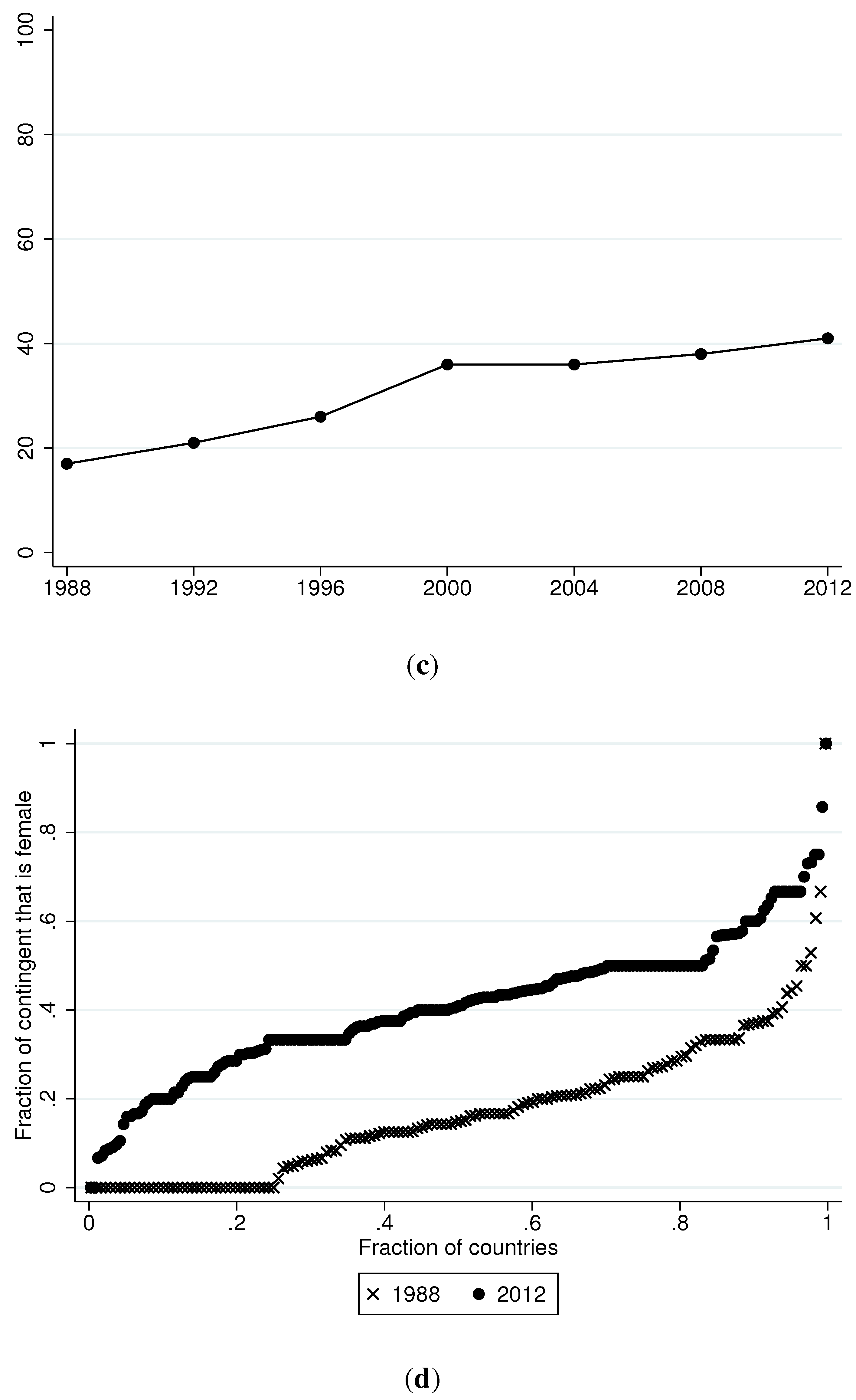
Our structural estimator requires that the three exclusions restrictions—PCGDP, population, and Islamic—affect medal winnings only indirectly through their impact on athletic contingents. To provide informal evidence of exclusion restriction validity, Figure 3 shows locally-weighted nonparameteric regressions of residuals from the outcome equation on each of the three exclusion restrictions. (The Figure uses residuals from Model 4, although residuals from Model 3 looked similar.) There appears to be a slight negative relationship between PCGDP and the residuals, which changes to a positive relationship at very high levels of PCGDP. However, the cluster of points does not seem to point to a significant relationship. The other two panels of Figure 3, which regress the residuals on population and Islamic, do not suggest a significant relationship. We interpret Figure 3 as supporting the validity of the exclusion restrictions. 6

Figure 3. Locally-weighted nonparameteric regressions of Model 4 residuals on the exclusion restrictions.

Figure 3. Locally-weighted nonparameteric regressions of Model 4 residuals on the exclusion restrictions.

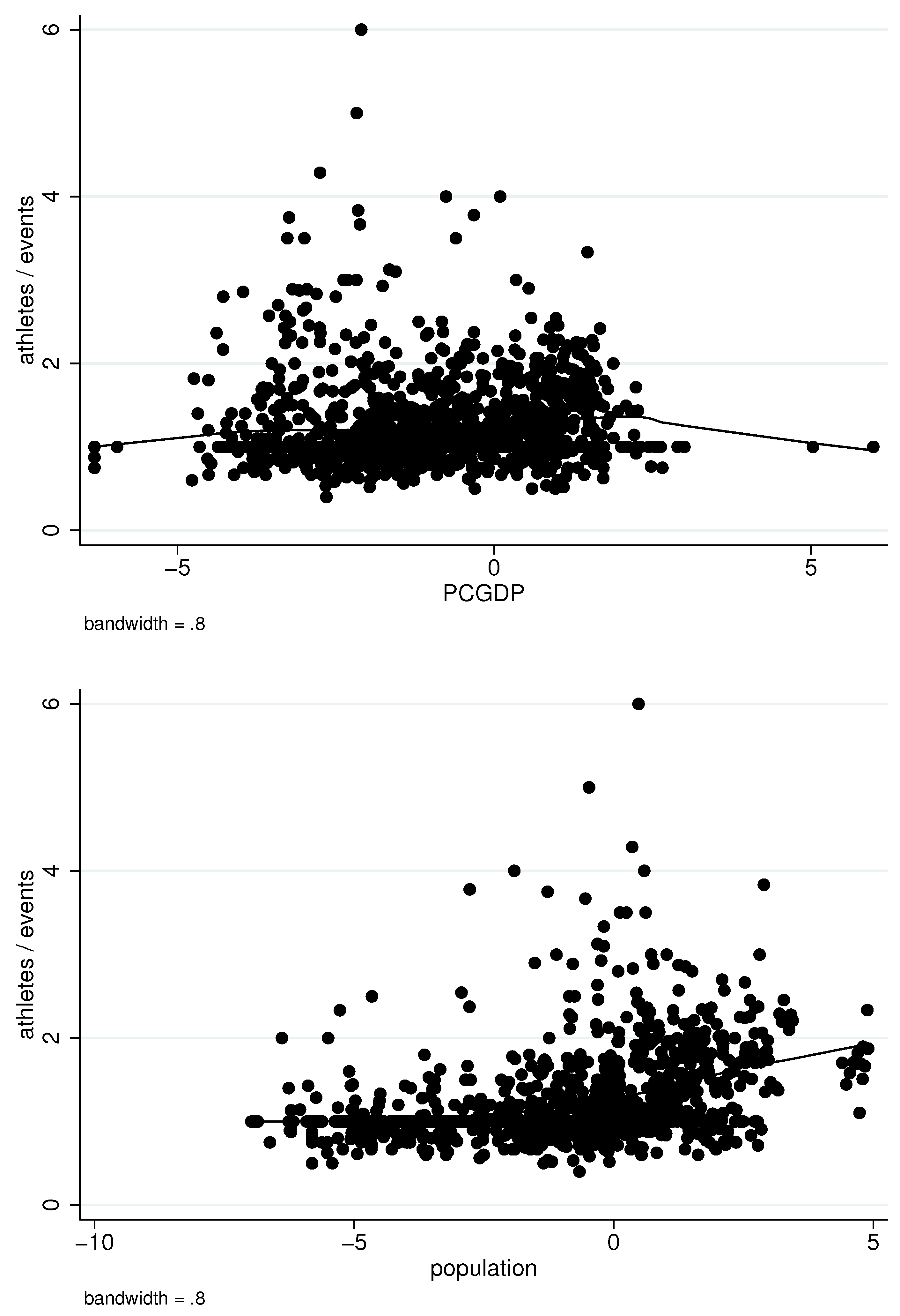
Nonetheless, because wealthy and/or large countries have access to resources not available to poorer and/or smaller countries, PCGDP and population might proxy for important missing explanatory variables, such as athlete quality. (Indeed, the following subsection shows that our models mis-fit winnings for several wealthy and/or large countries.) One potential explanation is that PCGDP and population might correlate with a country’s emphasis on individual versus team sports. Perhaps poorer/smaller countries focus on individual sports, as those tend to be less expensive to train for. In contrast, perhaps wealthier/larger countries, having access to more resources, emphasize relatively more expensive team sports.

To explore this conjecture, Figure 4 presents locally-weighted nonparametric regressions of athletes-per-events on PCGDP and population. While PCGDP does not appear to significantly correlate with athletes-per-events, the bottom panel does appear to point to a positive association between population and athletes-per-events, especially for the very largest countries. The implication is that larger countries appear to have resources that allow greater participation in team events.

Figure 4. Locally-weighted nonparametric regression of athletes/events on PCGDP and population.

Figure 4. Locally-weighted nonparametric regression of athletes/events on PCGDP and population.

6.3. Fitted Medal Winnings

We do not use our model to generate ex ante predicted medal winnings for two reasons. First, the model was not designed for prediction, but rather to identify the role of selection and endogeneity; in that sense it has a structural flavor. Second, if the main goal were prediction (conditional on aggregate information), then an approach simpler than that of this paper may be adequate. Testing for selection and/or endogeneity is unnecessary if one has no interest in identification of individual parameters and only the conditional prediction function is of interest. The goal then would be to simply focus on the prediction function. However, even in this case the predictor variables we have used above may be useful. This subsection considers some diagnostic devices for evaluating the in-sample fit of the model.

Writing the estimated regression as

$$ln\frac{{\widehat{s}}_{it}}{1-{\widehat{s}}_{it}}={\mathbf{x}}_{it}^{\prime }\widehat{\beta }+{\widehat{\epsilon }}_{it}$$

(10)

where $\mathbf{x}$ absorbs all regressors (including the selection and control function terms), and converting to an expression for ${\widehat{s}}_{it}$ gives

$${\widehat{s}}_{it}=\frac{(\frac{1}{N^{*}}{\sum }_{it}exp\left({\widehat{\epsilon }}_{it}\right))·exp\left({\mathbf{x}}_{it}^{\prime }\widehat{\beta }\right)}{(1+\frac{1}{N^{*}}{\sum }_{it}exp\left({\widehat{\epsilon }}_{it}\right))·exp\left({\mathbf{x}}_{it}^{\prime }\widehat{\beta }\right)}$$

(11)

where $N^{*}$ denotes the effective sample size and $\frac{1}{N^{*}}{\sum }_{it}exp\left({\widehat{\epsilon }}_{it}\right)$ is the sample average value of the residual, also known as the “smearing factor ” [28]. Multiplying ${\widehat{s}}_{it}$ by the total number of medals awarded yields the fitted number of medals.

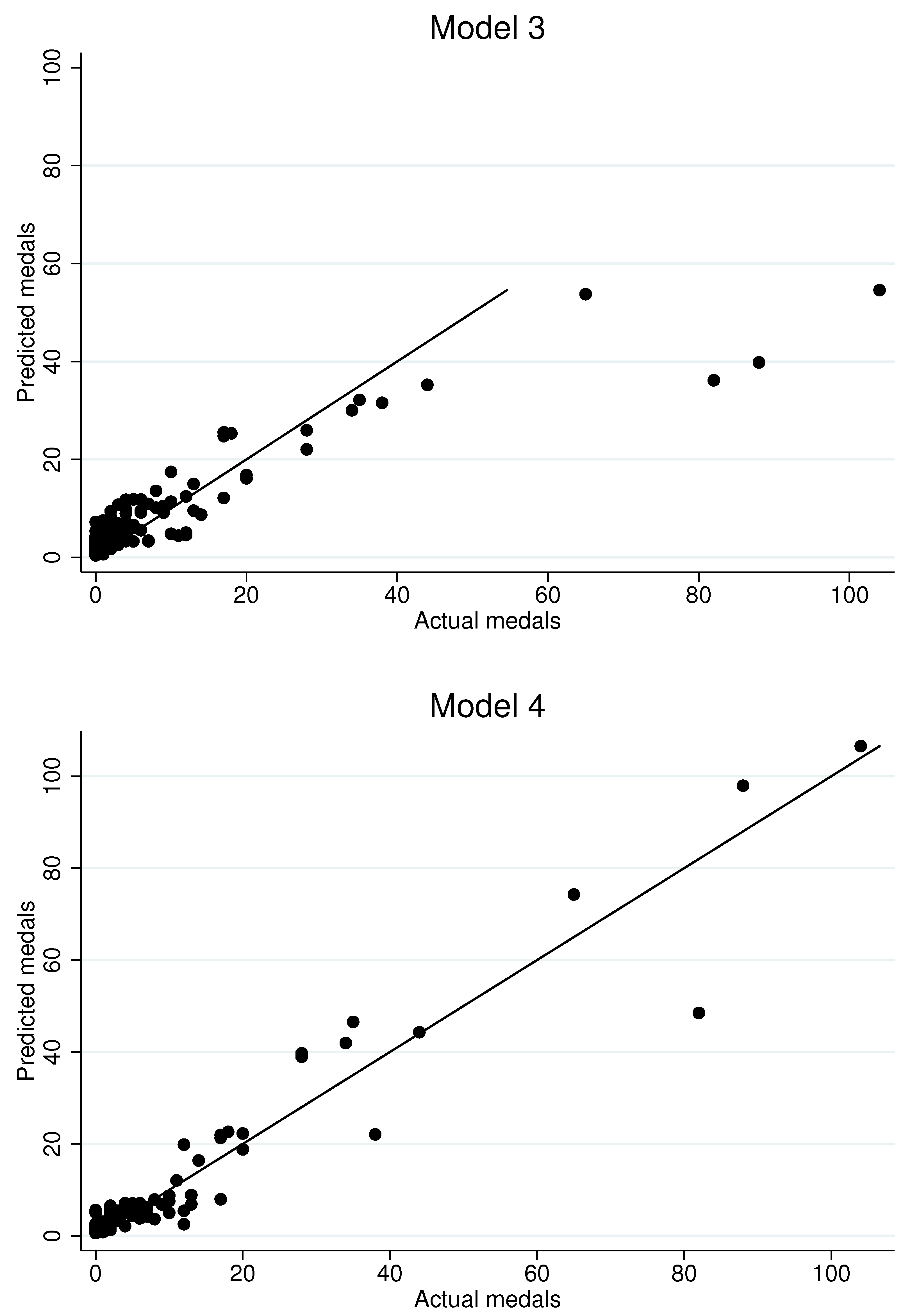
Figure 5 generates in-sample fitted values for the 2012 Olympiad in London based on the first four models in Table 14. Not surprisingly, although the inclusion of the control function does alter some of the coefficient estimates, it does not appear to substantially impact fitted values. The dynamic specification appears to offer the better fit, especially in the upper parts of the distribution of medals won, where the random effects approach appears to under-estimate the performance of countries that win many medals. We interpret this as evidence that the dynamic specification more accurately captures the influence of country-specific unobserved heterogeneity.

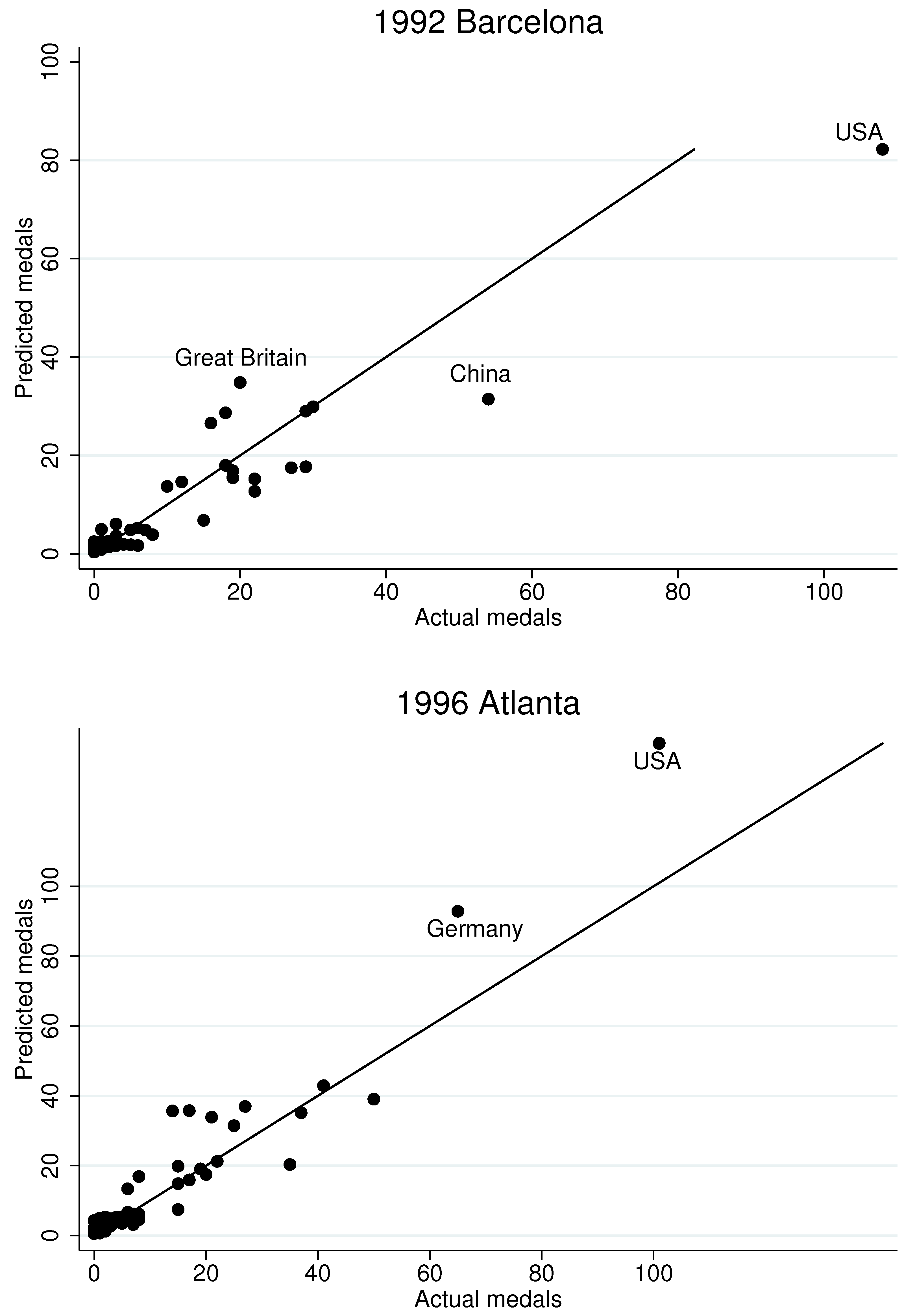
However, even our dynamic model appears to miss the performance of some countries. To gain a sense of which countries we miss and why, Figure 6 presents fitted values, based on the regression Model 4 in Table 14, for the last six Olympiads, with important “misses” labeled by country name. The London part of the figure repeats the last panel of Figure 5. Although the model appears to produce similar fits across all six Olympiads, several noteworthy results do emerge. First, the model under-estimates Russia’s performance in 2000 and 2012, but it over-estimates it in 2008. This may be largely due to the fact that Russia, as it is currently defined, did not participate in the first two Olympiads in our data. (It participated as the Soviet Union in 1988, and as part of a group of nations called the “Unified Team” in 1992.) Consequently, our Russian panel is shorter than panels for other countries, which likely skews estimates in our dynamic specification. Along similar lines, we struggle to fully capture the ascendancy of China in 1992. Other notable “misses” include Great Britain and the USA at the 1992 Barcelona games, Germany at the 1996 Atlanta games, and Japan for the past three Olympiads.

Figure 5. Actual and predicted medals in 2012 Olympiad.

Figure 5. Actual and predicted medals in 2012 Olympiad.

Figure 6. Actual and predicted medals in last six Olympiads.

Figure 6. Actual and predicted medals in last six Olympiads.

It is also noteworthy that we over-estimate the performance of some host countries. For example, we over-estimate medals for the USA in the 1996 Atlanta games, for Australia in the 2000 Sydney games, and for Greece in the 2000 Athens games. The reason for the over-estimates appears to stem from the unusually large athletic contingents those countries fielded during their host years. For example, in 2004 Greece more than tripled the size of its contingent compared to the previous Olympiad. Evidently, whether for public relations reasons or inexpensive travel costs, some host countries field athletes with lower chances of winning. On the other hand, despite China hosting in 2008 and fielding a large contingent, we under-estimate China’s performance in that year.

7. Conclusions

Previous economic studies of Olympic success have attempted to model medal winnings as dependent on GDP and population size. Although certainly important for predictive purposes, a more structural view of Olympic success interprets those variables as inputs into the process of producing athletes, who, in turn, compete to win medals. This paper presents an econometric model for considering such a setup, while also addressing econometric complications due to the nature of Olympic performance data.

Our results also indicate that, although it is possible to explain part of Olympiad success in terms of observed and unobserved country-specific traits, a significant random component remains. Some of this randomness relates to the unpredictable nature of sports, but some of this randomness is also due to countries that, for whatever reason, experience sudden success (or loss), and then manage to maintain that success (or lack thereof) at subsequent Olympiads.

Although generating accurate fits of medal winnings is not our stated goal, our model appears to perform satisfactorily for that purpose. We do appear to struggle to capture performance of countries in the midst of rapid political or economic transitions, notably Russia and China, and we also struggle to fully account for the impact that hosting has on winnings, evidently because some host countries inflate the size of their athletic contingents with competitors who have lower chances of success.