Article

Heteroskedasticity of Unknown Form in Spatial Autoregressive Models with a Moving Average Disturbance Term

Program in Economics, The Graduate School and University Center, The City University of New York, New York, NY 10016, USA
Econometrics 2015, 3(1), 101-127; https://doi.org/10.3390/econometrics3010101
Submission received: 14 October 2014 / Accepted: 27 January 2015 / Published: 26 February 2015
(This article belongs to the Special Issue Spatial Econometrics)

Abstract

:
In this study, I investigate the necessary condition for the consistency of the maximum likelihood estimator (MLE) of spatial models with a spatial moving average process in the disturbance term. I show that the MLE of spatial autoregressive and spatial moving average parameters is generally inconsistent when heteroskedasticity is not considered in the estimation. I also show that the MLE of parameters of exogenous variables is inconsistent and determine its asymptotic bias. I provide simulation results to evaluate the performance of the MLE. The simulation results indicate that the MLE imposes a substantial amount of bias on both autoregressive and moving average parameters.

1. Introduction

The spatial dependence among the disturbance terms of a spatial model is generally assumed to take the form of a spatial autoregressive process. The spatial model that has a spatial lag in the dependent variable and an autoregressive process in the disturbance term is known as the SARARmodel. The main characteristic of an autoregressive process is that the effect of a location-specific shock transmits to all other locations with its effects gradually fading away for the higher order neighbors. The spatial autoregressive process may not be appropriate if there is strong evidence of the localized transmission of shocks. That is, the autoregressive process is not the correct specification when the effects of shocks are contained within a small region and are not transmitted to other regions. An alternative to an autoregressive process is a spatial moving average process, where the effects of shocks are more localized. Haining [1], Anselin [2] and, more recently, Hepple [3] and Fingleton [4,5] consider a spatial moving average process for the disturbance terms. The spatial model that contains a spatial lag of the dependent variable and a spatial moving average process for the disturbance term is known as the SARMA model.
In the literature, various estimation methods have been proposed [6,7,8,9,10,11,12,13,14,15,16]. The ML method is the best known and most common estimator used in the literature for both SARAR and SARMA specifications. Lee [11] shows the first order asymptotic properties of the MLE for the case of SARAR(1,0). The generalized method of moment (GMM) estimators is also considered for the estimation of the spatial models. Kelejian and Prucha [6,7] suggest a two-step GMM estimator for the SARAR(1,1) specification. One disadvantage of the two-step GMME is that it is usually inefficient relative to the MLE [10,17,18].
To increase efficiency, Lee [12], Liu et al. [10] and Lee and Liu [13] formulate one-step GMMEs based on a set of moment functions involving linear and quadratic moment functions. In this approach, the reduced form of spatial models motivates the formulation of moment functions. The reduced equations indicate that the endogenous variable, i.e., the spatial lag term, is a function of a stochastic and a non-stochastic term. The linear moment functions are based on the orthogonality condition between the non-stochastic term and the disturbance term, while the quadratic moment functions are formulated for the stochastic term. Then, the parameter vector is estimated simultaneously with a one-step GMME. Lee [12] shows that the one-step GMME can be asymptotically equivalent to the MLE when disturbance terms are i.i.d. normal. In the case where disturbances are simply i.i.d., Liu et al. [10] and Lee and Liu [13] suggest a one-step GMME that can be more efficient than the (quasi) MLE.
Fingleton [4,5] extend the two-step GMME suggested by Kelejian and Prucha [6,7] for spatial models that have a moving average process in the disturbance term, i.e., SARMA(1,1). Baltagi and Liu [19] modify the moment functions considered in Fingleton [4] in the manner of Arnold and Wied [20] and suggest a GMME for the case of SARMA(0,1). The spatial moving average parameter in both Fingleton [4] and Baltagi and Liu [19] is estimated by a non-linear least squares estimator (NLSE). The asymptotic distribution for the NLSE of the spatial moving average parameter is not provided in either Fingleton [4] or Baltagi and Liu [19]. Recently, Kelejian and Prucha [9] and Drukker et al. [21] provided a basic theorem regarding the asymptotic distribution of their estimator under fairly general conditions. The estimation approach suggested in Kelejian and Prucha [9] and Drukker et al. [21] can easily be adapted for the estimation of the SARMA(1,1) and SARMA(0,1) models. Finally, although the Kelejian and Prucha approach in Fingleton [4] and Baltagi and Liu [19] has computational advantages, it may be inefficient relative to the ML method 1.
In the presence of an unknown form of heteroskedasticity, Lin and Lee [22] show that the MLE for the case of SARAR(1,0) may not be consistent, as the log-likelihood function is not maximized at the true parameter vector. They suggest a robust GMME for the SARAR(1,0) specification by modifying the moment functions considered in Lee [12]. Likewise, Kelejian and Prucha [9] modify the moment functions of their previous two-step GMME to allow for an unknown form of heteroskedasticity.
The spatial moving average model introduces a different interaction structure. Therefore, it is of interest to investigate the implications of a moving average process for estimation and testing issues. In this paper, I investigate the effect of heteroskedasticy on the MLE for the case of SARMA(1,1) and SARMA(0,1) along the lines of Lin and Lee [22]. The analytical results show that when heteroskedasticity is not considered in the estimation, the necessary condition for the consistency of the MLE is generally not satisfied for both the SARMA(1,1) and SARMA(0,1) models. For the SARMA(1,1) specification, I also show that the MLE of other parameters is also inconsistent, and I determine its asymptotic bias. My simulation results indicate that the MLE imposes a substantial amount of bias on spatial autoregressive and moving average parameters. However, the simulation results also show that the MLE of other parameters reports a negligible amount of bias in large samples.
The rest of this paper is organized as follows. In Section 2, I specify the SARMA(1,1) model in more detail and list assumptions that are required for the asymptotic analysis. In Section 3, I briefly discuss the implications of the spatial processes proposed for the disturbance term in the literature. Section 4 investigates the necessary condition for the consistency of the MLE of the autoregressive and moving average parameters. Section 5 provides expressions for the asymptotic bias of the MLE of parameters of the exogenous variables. Section 6 contains a small Monte Carlo simulation. Section 7 closes with concluding remarks.

2. Model Specification and Assumptions

In this study, the following first order SARMA(1,1) specification is considered:
Y n = λ 0 W n Y n + X n β 0 + u n , u n = ε n - ρ 0 M n ε n
where Y n is an n × 1 vector of observations of the dependent variable, X n is an n × k matrix of non-stochastic exogenous variables, with an associated k × 1 vector of population coefficients β 0 , W n , M n are n × n spatial weight matrices of known constants with zero diagonal elements and ε n is an n × 1 vector of disturbances. The variables W n Y n and M n ε n are known as the spatial lag of the dependent variable and the disturbance term, respectively. The spatial effect parameters λ 0 and ρ 0 are known as the spatial autoregressive and moving average parameters, respectively. As the spatial data are characterized with triangular arrays, the variables in Equation (1) have subscript n 2. The model specifications with λ 0 0 , ρ 0 0 and λ 0 = 0 , ρ 0 are known, respectively, as SARMA(1,1) and SARMA(0,1) in the literature. Let Θ be the parameter space of the model. In order to distinguish the true parameter vector from other possible values in Θ, the model is stated with the true parameter vector θ 0 = β 0 , δ 0 with δ 0 = λ 0 , ρ 0 .
For notational simplicity, I denote S n λ = I n - λ W n , R n ( ρ ) = I n - ρ M n , G n ( λ ) = W n S n - 1 ( λ ) , H n ( ρ ) = M n R n - 1 ( ρ ) , X ¯ n ( ρ ) = R n - 1 ( ρ ) X n , and G ¯ n ( δ ) = R n - 1 ( ρ ) G n ( λ ) R n ( ρ ) . Furthermore, at the true parameter values ( ρ 0 , λ 0 ) , I denote S n ( λ 0 ) = S n , R n ( ρ 0 ) = R n , G n ( λ 0 ) = G n , H n ( ρ 0 ) = H n , X ¯ n ( ρ 0 ) = X ¯ n and G ¯ n ( δ 0 ) = G ¯ n .
The model in Equation (1) is considered under the following assumptions.
Assumption 1. 
The elements ε n i of the disturbance term ε n are distributed independently with mean zero and variance σ n i 2 and E ε n i ν < for some ν > 4 for all n and i.
The elements of the disturbance term have moments higher than the fourth moment. The existence moments condition is required for the application of the central limit theorem for the quadratic form given in Kelejian and Prucha [9]. In addition, the variance of a quadratic form in ε n exists and is finite when the first four moments are finite. Finally, Liapunov’s inequality guarantees that the moments less than ν are also uniformly bounded for all n and i.
Assumption 2. 
The spatial weight matrices M n and W n are uniformly bounded in absolute value in row and column sums. Moreover, S n - 1 , S n - 1 ( λ ) , R n - 1 and R n - 1 ( ρ ) exist and are uniformly bounded in absolute value in row and column sums for all values of ρ and λ in a compact parameter space.
The uniform boundedness of the terms in Assumption 2 is motivated to control spatial autocorrelations in the model at a tractable level [6] 3. Assumption 2 also implies that the model in Equation (1) represents an equilibrium relation for the dependent variable. By this assumption, the reduced form of the model becomes feasible as Y n = S n - 1 X n β 0 + S n - 1 R n ε n . The uniform boundedness of S n - 1 ( λ ) and R n - 1 ( ρ ) in Assumption 2 is only required for the MLE, not for the GMME [10]. When W n is row normalized, a closed subset of interval ( 1 / λ m i n , 1 ) , where λ m i n is the smallest eigenvalue of W n , can be considered as the parameter space for λ 0 . Analogously, a closed subset of ( 1 / ρ m i n , 1 ) , where ρ m i n is the smallest eigenvalue of M n , can be the parameter space of ρ 0 ([15], p.128) 4.
The next assumption states the regularity conditions for the exogenous variables.
Assumption 3. 
The matrix X n is an n × k matrix consisting of constant elements that are uniformly bounded. It has full column rank k. Moreover, lim n 1 n X n X n and lim n 1 n X ¯ n ( ρ ) X ¯ n ( ρ ) exist and are nonsingular for all values of ρ in a compact parameter space.

3. Spatial Processes for the Disturbance Term

In the literature, there are three main parametric processes to model spatial autocorrelation among disturbance terms: (i) the spatial autoregressive process (SAR); (ii) the spatial moving average process (SMA); and (iii) the spatial error components model (SEC). The implied covariance structure is different under each specification. In this section, I describe the transmission and the effect of shocks under each specification. The SAR process is specified as:
u n = ρ 0 M n u n + ε n
where u n is an n × 1 vector of regression disturbances and ε n is an n × 1 vector of i.i.d. innovations with variance σ 0 2 . Under the assumption of an equilibrium, i.e., R n is invertible, the reduced from of Equation (2) is u n = R n - 1 ε n with the covariance matrix of E u n u n = Ω n = σ 0 2 R n - 1 R n - 1 . Note that even if the innovations are homoskedastic, the diagonal elements of Ω n are not equal, suggesting heteroskedasticity for the regression disturbances. An expansion of ( I n - ρ 0 M n ) - 1 for | ρ 0 | < 1 yields ( I n - ρ 0 M n ) - 1 = j = 0 ρ 0 j M n j = I n + ρ 0 M n + ρ 0 2 M n 2 + . Hence, the SAR specification of the disturbance term implies that a shock at location i is transmitted to all other locations. The first term I n implies that the shock at location i directly affects location i and, through other terms denoted by the powers of M n , affects higher order neighbors. Eventually, the shock feeds back to location i through the interconnectedness of neighbors. Note that | ρ 0 | < 1 ensures that the magnitude of the transmitted shock decreases for the higher orders of neighbors. As a result, the SAR specification allows researchers to model the global transmission of shocks where the full effect of a shock to location i is the sum of the initial shock and the feedback from other locations.
If a more localized spatial dependence is conjectured for an economic model, then a spatial moving average process (SMA) specification is more suitable [1,3,4,5]. The SMA process is specified as:
u n = ε n - ρ 0 M n ε n
where ρ 0 is the spatial moving average parameter. The reduced form does not involve an inverse of a square matrix. Hence, the transmission of a shock emanated from location i is limited to its immediate neighbors given by the nonzero elements in the i-th row of M n . Under this specification, the covariance matrix of u n is Ω n = σ 0 2 R n R n = σ 0 2 I n - ρ 0 ( M n + M n ) + ρ 0 2 M n M n . The spatial covariance is limited to nonzero elements of M n + M n and M n M n . In comparison with the SAR specification, the range of covariance induced by the SMA model is much smaller.
Kelejian and Robinson [23] suggest another specification, which is called the spatial error components (SEC) model. This specification is similar to the SMA process in the sense that the implied covariance matrix does not involve a matrix inverse. Formally, the SEC model is given by u n = M n ε n + ϵ n , where ε n is an n × 1 vector of regional innovations, whereas ϵ n is an n × 1 vector of locational innovations. Assuming that ε n and ϵ n are independent, the variance-covariance matrix becomes Ω n = σ ϵ 2 I n + σ ε 2 M n M n , which indicates that the spatial correlation in a SEC specification is even more localized.
There have been some direct attempts to parametrize the covariance matrix of u n , rather than defining a process for the disturbance term. For example, Besag [24] considers a conditional first-order autoregressive model (CAR(1)), such that the covariance matrix of u n takes the form of Ω n = σ 0 2 ( I n - ρ 0 M n ) - 1 , where M n is assumed to be a symmetric contiguity matrix. This covariance structure implies a process of u n = ( I n - ρ 0 M n ) - 1 / 2 ε n . As in the case of the SAR process, a shock in a location is transmitted to all other locations, but now with a smaller amplitude. Another example is Ω n = σ 0 2 ( I n + ρ 0 M n ) , where M n is assumed to be symmetric [25,26]. In this case, the spatial correlation is restricted to first order neighbors, i.e., non-zero elements of M n .
The elements of Ω n can also be specified through a covariance generating function. For example, in Ripley [27], the covariance generating function is defined in terms of the distance between two locations in such a way that the resulting covariance is always non-negative definite. Let d i j be the distance between locations i and j and Ω i j , n be the covariance between these two locations. Then, the covariance generating function is defined by:
Ω i j , n = σ 0 2 2 n cos - 1 ( d i j 2 ψ ) - d i j 2 ψ ( 1 - d i j 2 4 ψ 2 ) 1 / 2 , if d i j 2 ψ 0 , otherwise .
Intuitively, Ω i j , n is proportional to the intersection area of two discs of common radius centered on locations i and j. The covariance generating function in Equation (4) depends on the single parameter ψ and has a fairly linear negative relationship with d i j [25,27]. Another covariance generating function family, first introduced by Whittle in 1954, is a two-parameter function defined in terms of gamma and bessel functions. This family has the following specification:
Ω i j , n = σ 0 2 2 ν - 1 Γ ( ν ) - 1 ( δ d i j ) ν K ν ( δ d i j )
where K ν ( · ) is the modified bessel function and Γ ( · ) is the standard gamma function. The parameters ν > 0 and δ > 0 are respectively known as a shape parameter and a spatial parameter. The spatial parameter δ determines how far the spatial correlation will stretch. For the special case, where ν = 1 2 , this covariance generating function gives an exponential decaying spatial correlation [25]. There is also a more general exponential covariance generating function that depends on two parameters. This function is specified by Ω i j , n = σ 0 2 γ exp ( λ d i j ) , where γ and λ are parameters that need to be estimated. This function also exhibits exponential decay for the spatial correlations.
In the literature, there are some other covariance generating function families. However, the majority of these functions do not necessarily ensure that Ω n is a positive-definite matrix [25,28]. The formal properties of the MLE for spatial models that have a covariance structure determined by a parametric function are investigated in an early study by Mardia and Marshall [29]. In this study, the authors state conditions under which the MLE is consistent and has an asymptotic normal distribution.
In this study, the spatial model specified in Equation (1) is considered. The interaction between the spatial autoregressive process and the moving average process for this model induces a complicated pattern for the transmission of a location-specific shock. Under Assumption 2, the reduced form of the model is given by Y n = S n - 1 X n β 0 + S n - 1 R n ε n . The last term in the reduced form can be written as S n - 1 R n ε n = ε n - ρ 0 M n ε n + l = 1 λ 0 l W n l ε n - ρ 0 M n l = 1 λ 0 l W n l ε n . In this representation, the higher power of W n does not have zero diagonal elements, which, in turn, implies that the total effect of a region-specific shock also contains the feedback effects passed through other locations. The corresponding expression in the case of SARAR(1,1) specification is given by S n - 1 R n - 1 ε n = l = 0 λ 0 l W n l k = 0 ρ 0 k M n k ε n . Again, the induced pattern involves the interaction of two weight matrices and two parameters.
Following Fingleton [4], I illustrate the transmission pattern for a shock under each specification by using a rook weight matrix over a 15 × 15 lattice. Figure 1 shows the impact of a shock emanated from the unit located at the center of lattice 5. In the case of SAR and SARAR(1,1), the effect of shock is more vigorous over the whole lattice. For the SMA specification, the shock is only transmitted to the immediate units, as shown in Figure 1b. In contrast, the effect of the shock gradually dies out under the SARMA(1,1) model.
Figure 1. The effect of a shock. (a) The effect of a shock: spatial autoregressive process (SAR). (b) The effect of a shock: spatial moving average process (SMA). (c) The effect of a shock: SARAR(1,1). (d) The effect of a shock: SARMA(1,1).
Econometrics 03 00101 g001

4. The MLE of λ 0 and ρ 0

The log-likelihood function for the model in Equation (1) under the assumption that the disturbance terms of the model are i.i.d. normal with mean zero and variance σ 0 2 can be written as:
ln L n ( ζ ) = - n 2 ln ( 2 π ) - n 2 ln ( σ 2 ) + ln S n ( λ ) - ln R n ( ρ )
- 1 2 σ 2 S n ( λ ) Y n - X n β R n - 1 ( ρ ) R n - 1 ( ρ ) S n ( λ ) Y n - X n β
where ζ = θ , σ 2 . The first order conditions with respect to β and σ 2 are respectively given by:
ln L n ( ζ ) β = 1 σ 2 X ¯ n ( ρ ) R n - 1 ( ρ ) S n ( λ ) Y n - X n β
ln L n ( ζ ) σ 2 = - n 2 σ 2 + 1 2 σ 4 ε n ( θ ) ε n ( θ )
where ε n ( θ ) = R n - 1 ( ρ ) S n ( λ ) Y n - X n β . The solutions of the first order conditions for a given δ yield the MLE of β 0 and σ 0 2 :
β ^ n ( δ ) = X ¯ n ( ρ ) X ¯ n ( ρ ) - 1 X ¯ n ( ρ ) R n - 1 ( ρ ) S n ( λ ) Y n
σ ^ n 2 ( θ ) = 1 n ε n ( θ ) ε n ( θ )
Concentrating the log-likelihood function by eliminating σ 2 gives the following equation:
ln L n ( θ ) = - n 2 ln ( 2 π ) - 1 2 - n 2 ln ε n ( θ ) ε n ( θ ) | S n ( λ ) | 2 n | R n ( ρ ) | - 2 n
The above representation is useful for exploring the role of the Jacobian terms | S n ( λ ) | and | R n ( ρ ) | in the ML estimation. The MLE of θ is the extremum estimator obtained from the maximization of Equation (9). In an equivalent way, the MLE of θ 0 can be defined by:
θ ^ n = argmin θ Θ ε n ( θ ) ε n ( θ ) | S n ( λ ) | 2 n | R n ( ρ ) | - 2 n
In the special case, where | S n ( λ ) | = | R n ( ρ ) | = 1 , the MLE is the NLSE obtained from the minimization of ε n ( θ ) ε n ( θ ) , i.e., θ ^ N L S E , n = argmin θ Θ ε n ( θ ) ε n ( θ ) . It is clear that the Jacobian terms | S n ( λ ) | and | R n ( ρ ) | play the role of a weight (or a penalty) on ε n ( θ ) ε n ( θ ) . The penalty is a function of the autoregressive parameters and the spatial weight matrices, which can be defined as f λ , ρ , W n , M n = S n ( λ ) 2 n R n ( ρ ) - 2 n . For the SARAR(1,1) specification, the last term in Equation (9) is given by - n 2 ln ε n ( θ ) ε n ( θ ) S n ( λ ) 2 n R n ( ρ ) 2 n , where ε n ( θ ) = R n ( ρ ) S n ( λ ) Y n - X n β . Therefore, in the case of SARAR(1,1), the MLE of θ 0 is given by:
θ ^ n = argmin θ Θ ε n ( θ ) ε n ( θ ) | S n ( λ ) | 2 n | R n ( ρ ) | 2 n
It is hard to make any general statement about the effects and magnitudes of the penalty functions in both cases. Hepple [30] illustrates that the Jacobian term imposes a substantial penalty for the SARAR(0,1) specification. To illustrate the effect of penalty functions for the case of SARMA(1,1) and SARAR(1,1), I use a distance-based weight matrix for a sample of 91 countries, such that each country is connected to every other country. The elements of the weight matrices are specified by:
w i j = m i j = 0 if i = j d i j - 2 j = 1 91 d i j - 2 if i j
where d i j between countries i and j is measured by the great circle distance between country capitals 6. Figure 2 shows the surface plots of penalty functions over a grid of spatial parameters.
Figure 2. The penalty functions for the dense weight matrix. (a) The penalty function for SARMA(1,1). (b) The penalty function for SARAR(1,1).
Econometrics 03 00101 g002
For the SARAR(1,1) specification, the value of the penalty function decreases as the parameter combination ( λ , ρ ) moves away from ( 0 , 0 ) in any direction, as shown in Figure 2b 7. On the other hand, there is no such monotonic decrease in the penalty function under the SARMA(1,1) specification, as illustrated in Figure 2a. The penalty function of SARMA(1,1) obtains relatively larger values when there is strong spatial dependence in the disturbance term, i.e., when ρ is near + 1 or - 1 . In contrast, the penalty function has smaller values when there is strong spatial dependence in the dependent variable. This pattern indicates that the sum ε n ( θ ) ε n ( θ ) is penalized as ρ moves toward either + 1 or - 1 . In the case of SARAR(1,1), this sum gets larger as ( λ , ρ ) moves toward ( ± 1 , ± 1 ) in any direction, suggesting that the solution of the minimization problem is restricted to the region ( - 1 , - 1 ) × ( + 1 , + 1 ) . Finally, in a small neighborhood of ( 0 , 0 ) , the surface plots in Figure 2 indicate that the penalty functions take values around one, suggesting that the parameter estimates from the MLE can be similar to those from the NLSE under both specifications.
Next, I investigate the effect of heteroskedasticity on the MLE for the case of SARMA(1,1). I assume that the true data generating process is characterized by Assumption 1. More explicitly, the MLE σ ^ n 2 ( δ ) can be written as:
σ ^ n 2 ( δ ) = 1 n Y n S n ( λ ) R n - 1 ( ρ ) M ¯ n ( ρ ) R n - 1 ( ρ ) S n ( λ ) Y n
where M ¯ n ( ρ ) = I n - P n ( ρ ) is a projection-type matrix with P n ( ρ ) = X ¯ n ( ρ ) X ¯ n ( ρ ) X ¯ n ( ρ ) - 1 X ¯ n ( ρ ) . Substituting R n - 1 ( ρ ) S n ( λ ) Y n = R n - 1 ( ρ ) X n β + ε n into σ ^ n 2 ( δ ) and using the fact that X ¯ n ( ρ ) M ¯ n ( ρ ) = 0 k × n and M ¯ n ( ρ ) X ¯ n ( ρ ) = 0 n × k , the MLE σ ^ n 2 ( δ ) can be written as:
σ ^ n 2 ( δ ) = 1 n ε n M ¯ n ( ρ ) ε n
At δ 0 , the probability limit of σ ^ n 2 ( δ 0 ) is:
plim n σ ^ n 2 ( δ 0 ) = plim n 1 n ε n ε n - plim n 1 n 2 ε n X ¯ n 1 n X ¯ n X ¯ n - 1 X ¯ n ε n
For the first term on the right-hand side, we have 1 n ε n ε n = 1 n i = 1 n σ n i 2 + o p ( 1 ) by Chebyshev’s weak law of large numbers. The second term vanishes by virtue of Lemma 1(4) in Appendix A and Assumption 3. Therefore, we have:
σ ^ n 2 ( δ 0 ) = 1 n i = 1 n σ n i 2 + o p ( 1 )
The result in Equation (16) indicates that the average of the individual variances is asymptotically equivalent to σ ^ n 2 ( δ 0 ) .
Concentrating out β and σ 2 from the log-likelihood function in Equation (6) yields:
ln L n ( δ ) = - n 2 ( ln ( 2 π ) + 1 ) - n 2 ln σ ^ n 2 ( δ ) + ln S n ( λ ) - ln R n ( ρ )
The MLEs λ ^ n and ρ ^ n are extremum estimators obtained from the maximization of Equation (17). The first order conditions of Equation (17) with respect to ρ and λ are 8:
ln L n ( δ ) λ = - n 2 σ ^ n 2 ( δ ) σ ^ n 2 ( δ ) λ - tr G n ( λ )
ln L n ( δ ) ρ = - n 2 σ ^ n 2 ( δ ) σ ^ n 2 ( δ ) ρ + tr H n ( ρ )
where G n ( λ ) = W n S n - 1 ( λ ) and H n ( ρ ) = M n R n - 1 ( ρ ) . For the consistency of λ ^ n and ρ ^ n , the necessary condition is plim n 1 n ln L n ( δ 0 ) δ = 0 . Below, I investigate the probability limit of the following expression:
1 n ln L n ( δ 0 ) δ = 1 n - n 2 n ε n M ¯ n ε n σ ^ n 2 ( δ 0 ) λ - 1 n tr G n 1 n - n 2 n ε n M ¯ n ε n σ ^ n 2 ( δ 0 ) ρ + 1 n tr H n
Under Assumption 2, both H n and G n are uniformly bounded in absolute value in row and column sums. Therefore, 1 n tr H n and 1 n tr G n in Equation (19) are of order O ( 1 ) . With these results for 1 n tr H n and 1 n tr G n , a convenient result for the probability limit of Equation (19) can be obtained, which is stated in the following proposition.
Proposition 1. 
Under Assumptions 1 through 3, we have:
1 n ln L n ( δ 0 ) δ = Cov G ¯ n , i i , σ n i 2 σ ¯ 2 + o p ( 1 ) - Cov H n , i i , σ n i 2 σ ¯ 2 + o p ( 1 )
where Cov G ¯ n , i i , σ n i 2 is the covariance between the diagonal elements of G ¯ n , { G ¯ n , 11 , G ¯ n , 22 , , G ¯ n , n n } and the individual variances { σ n 1 2 , σ n 2 2 , , σ n n 2 } . Similarly, Cov H n , i i , σ n i 2 denotes the covariance between diagonal elements of H n , { H n , 11 , H n , 22 , , H n , n n } and the individual variances { σ n 1 2 , σ n 2 2 , , σ n n 2 } .
Proof. 
See Appendix B. ▢
The above proposition indicates that the MLE of the spatial autoregressive and moving average parameters is not consistent, as long as the covariance terms in Equation (20) are not zero. Notice that, when the disturbance terms are homoskedastic, the covariance terms in Equation (40) are zero. In the special case where W n = M n and λ 0 = ρ 0 , we have S n = R n and G n = H n , so that G ¯ n = R n - 1 G n R n = R n - 1 H n R n = R n - 1 M n R n - 1 R n = H n . Hence, the necessary condition for the consistency of λ ^ n is identical to the one for ρ ^ n .
The result in Proposition 1 indicates that the consistency of the MLE depends on the specification of weight matrices. It is of interest to investigate specifications that yield zero covariances. An obvious case is when there is no variation in the diagonal elements of G ¯ n and H n . Then, the necessary condition for the consistency of λ ^ n and ρ ^ n is not violated, even if the disturbances are heteroskedastic. For example, there is no variations in the diagonal elements of G ¯ n and H n when W n and M n are block-diagonal matrices with an identical sub-matrix in the diagonal blocks and zeros elsewhere. This type of block diagonal weight matrix can be seen in social interaction scenarios where a block represents a group in which each individual is equally affected by the members of the group [32,33]. Suppose that there are R groups, each of which has m members, so that n = m R . If we assign equal weight to each member of a group, then W n = M n = I R B m , where B m = 1 m - 1 l m l m - I m , and l m is an m-dimensional column vector of ones. For this setup, there is no variation in the diagonal elements of G ¯ n and H n ; therefore Cov G ¯ n , i i , σ n i 2 = Cov H n , i i , σ n i 2 = 0 .
There is also no variation in the diagonal elements of G ¯ n and H n when the circular world weight matrices considered in Kelejian and Prucha [7] are employed. In these weight matrices, the order of observations is important, since the observations are related to some units in front and to some in back. As an example, consider a “one ahead and one behind” weight matrix, where each observation is related to the one immediately after and immediately before it. For this scenario, we also have Cov G ¯ n , i i , σ n i 2 = Cov H n , i i , σ n i 2 = 0 . The circular world weight matrices can be adjusted to create some variation in the diagonal elements of G ¯ n and H n . For example, Kelejian and Prucha [34] construct a different version in which the first and the last one-third of the sample observations has five neighbors in front and five in back, while the middle third only has one neighbor in front and one in back. Under this scenario, the Monte Carlo results in Kelejian and Prucha [34] show that the MLE is significantly biased for the case of SARAR(1,1).

5. The MLE of β 0

In the previous section, I showed that the consistency of the MLE of the spatial autoregressive and moving average parameters is not ensured. In this section, I investigate the consistency of the MLE of β 0 . The result in Equation (8a) indicates that the MLE β ^ n ( δ ^ n ) is also inconsistent, since it is based on the inconsistent estimators λ ^ n and ρ ^ n . The asymptotic bias of β ^ n ( δ ^ n ) can be determined from Equation (8a). By using S n ( λ ) = S n + λ 0 - λ W n , the MLE β ^ n ( δ ) can be written as:
β ^ n ( δ ) = β 0 + X ¯ n ( ρ ) X ¯ n ( ρ ) - 1 X ¯ n ( ρ ) R n - 1 ( ρ ) R n ε n
+ λ 0 - λ X ¯ n ( ρ ) X ¯ n ( ρ ) - 1 X ¯ n ( ρ ) R n - 1 ( ρ ) G n X n β 0
+ λ 0 - λ X ¯ n ( ρ ) X ¯ n ( ρ ) - 1 X ¯ n ( ρ ) R n - 1 ( ρ ) G n R n ε n
Under Assumption 3, the term 1 n X ¯ n ( ρ ) X ¯ n ( ρ ) - 1 is uniformly bounded in absolute value in row and column sums. By Lemma 1(5) of Appendix A, terms involving ε n in Equation (21) vanish in probability. Thus,
β ^ n ( δ ) = β 0 + λ 0 - λ X ¯ n ( ρ ) X ¯ n ( ρ ) - 1 X ¯ n ( ρ ) R n - 1 ( ρ ) G n X n β 0 + o p ( 1 )
The asymptotic bias of β ^ n ( δ ^ n ) follows from Equation (22), which is given by λ 0 - λ ^ n X ¯ n ( ρ ^ n ) X ¯ n ( ρ ^ n ) - 1 X ¯ n ( ρ ^ n ) R n - 1 ( ρ ^ n ) G n X n β 0 . This result shows that the asymptotic bias of β ^ n ( δ ^ n ) depends on weight matrices and the regressors matrix and is not zero unless the spatial parameters are consistent. Note that the bias is the OLS estimator obtained from the artificial regression of R n - 1 ( ρ ^ n ) G n X n β 0 on X ¯ n ( ρ ^ n ) . For the special case of λ ^ n = λ 0 + o p ( 1 ) , we have β ^ n ( δ ) = β 0 + o p ( 1 ) . In this case, there is no asymptotic bias, and the inconsistency of ρ ^ n has no effect on β ^ n ( δ ^ n ) .
The specification with λ 0 = 0 in Equation (1) is called the spatial moving average model (SARMA(0,1) or SMA). For the SARMA(0,1) specification, the log-likelihood function simplifies to:
ln L n ( ζ ) = - n 2 ln ( 2 π ) - n 2 ln ( σ 2 ) - ln R n ( ρ ) - 1 2 σ 2 Y n - X n β R n - 1 ( ρ ) R n - 1 ( ρ ) Y n - X n β
where ζ = θ , σ 2 with θ = ρ , β . For a given value of ρ, the first order conditions yield:
β ^ n ( ρ ) = X ¯ n ( ρ ) X ¯ n ( ρ ) - 1 X ¯ n ( ρ ) R n - 1 ( ρ ) Y n
σ ^ n 2 ( ρ ) = 1 n ε n ( θ ) ε n ( θ )
where ε n ( θ ) = R n - 1 Y n - X ¯ n β . The necessary condition for the consistency of the MLE ρ ^ n can be obtained from Equation (20). From the second row of Equation (20), we have 1 n ln L n ( ρ 0 ) ρ = - Cov H n , i i , σ n i 2 σ ¯ 2 + o p ( 1 ) , which implies that the MLE ρ ^ n is inconsistent. Substitution of Y n = X n β 0 + R n ε n into β ^ n ( ρ ) yields:
β ^ n ( ρ ) = β 0 + X ¯ n ( ρ ) X ¯ n ( ρ ) - 1 X ¯ n ( ρ ) R n - 1 ( ρ ) ε n
The variance of X ¯ n ( ρ ) X ¯ n ( ρ ) - 1 X ¯ n ( ρ ) R n - 1 ( ρ ) R n ε n in Equation (24) has an order of O ( 1 n ) by Lemma 1(5) of Appendix A. Then, Chebyshev’s inequality implies that β ^ n ( ρ ) = β 0 + o p ( 1 ) . Hence, β ^ n ( ρ ^ n ) has no asymptotic bias, even though ρ ^ n is inconsistent.
For the spatial autoregressive model, where ρ 0 = 0 in Equation (1), the result in Equation (20) simplifies to 1 n ln L n ( λ 0 ) λ = Cov G n , i i , σ n i 2 σ ¯ 2 + o p ( 1 ) . The term X ¯ n ( ρ ) X ¯ n ( ρ ) - 1 X ¯ n ( ρ ) R n - 1 ( ρ ) G n X n β 0 in Equation (22) simplifies to X n X n - 1 X G n X n β 0 , so that:
β ^ n ( λ ) = β 0 + λ 0 - λ X n X n - 1 X G n X n β 0 + o p ( 1 )
The result in Equation (25) is the exact result stated in Lin and Lee [22] for the case of SARAR(1,0).
I collect the above results for the MLE of β 0 in the following proposition.
Proposition 2. 
Consider the model in Equation (1) under Assumptions 1 through 3; then:
(1)
For the SARMA(1,1) model, we have:
β ^ n ( δ ) = β 0 + λ 0 - λ X ¯ n ( ρ ) X ¯ n ( ρ ) - 1 X ¯ n ( ρ ) R n - 1 ( ρ ) G n X n β 0 + o p ( 1 )
(2)
For the SARMA(0,1) model, where λ 0 = 0 , we have β ^ n ( ρ ) = β 0 + o p ( 1 ) .
(3)
For the SARMA(1,0) model, where ρ 0 = 0 , we have:
β ^ n ( λ ) = β 0 + λ 0 - λ X n X n - 1 X G n X n β 0 + o p ( 1 )
In Section 4 and Section 5, I showed that the MLE of δ 0 and β 0 is generally inconsistent when heteroskedasticity is present in the model. Besides its computational burden, the consistency of MLE is not ensured. In the next section, I confirm these large sample results through a Monte Carlo simulation.

6. Monte Carlo Simulation

In this section, the finite sample properties of the MLE are investigated through a Monte Carlo experiment for the cases of (i) SARMA(0,1) and (ii) SARMA(1,1). For both models, I assume heteroskedastic innovations in the data generating processes.

6.1. Design

There are two regressors and no intercept term, such that X n = [ x n , 1 , x n , 2 ] and β 0 = ( β 10 , β 20 ) , where x n , 1 and x n , 2 are n × 1 independent random vectors that are generated from a Normal(0,1). I consider n = 100, 500, 1,000; let W n = M n , and set β 0 = ( 1 , 1 ) for all experiments. For the spatial autoregressive parameters ( λ 0 , ρ 0 ) , I employ combinations from the set B = - 0 . 6 , - 0 . 3 , 0 , 0 . 3 , 0 . 6 to allow for weak and strong spatial interactions.
The row normalized spatial weight matrix is based on the small group interaction scenario described in Lin and Lee [22]. In this scenario, the weight matrix is a block diagonal matrix where each block represents a group interaction. The size of each block is determined by the group size, which is determined by a random draw from Uniform(15,50). Let { g 1 , , g G } be the set of groups, where G is the total number of groups. Denote the size of each group by m i for i = 1 , , G . Then, the block for group i is given by B i = 1 m i - 1 l m i l m i - I m i , where l m i is the m i × 1 vector of ones. Then, W n = M n = Diag B 1 , , B G 9.
The observations in a group have the same variance, and I use the group size to create heteroskedasticity. If the group size is greater than 35, I set the variance of that group equal to its size raised to 0 . 4 power; otherwise I let the variance be the square of the inverse of the group size. Then, the i-th element of the innovation vector ε n is generated according to ε n i = σ n i ξ n i , where σ n i is the standard error for the i-th observation and ξ n i ’s are i.i.d. Normal(0,1).
I use the following expressions to measure the level of signal-to-noise in this setup [35]:
R S A R M A ( 1 , 1 ) 2 = 1 - tr R n S n - 1 S n - 1 R n Σ n β 0 X n S n - 1 S n - 1 X n β 0 + tr R n S n - 1 S n - 1 R n Σ n
R S A R M A ( 0 , 1 ) 2 = 1 - tr R n R n Σ n β 0 X n X n β 0 + tr R n R n Σ n
where Σ n is the diagonal n × n covariance matrix of the disturbance terms. This setup yields an R 2 value close to 0 . 55 . For each specification, the Monte Carlo experiment is based on 1,000 repetitions.

6.2. Simulation Results

The simulation results are presented in Appendix C and Appendix D. In each table, the empirical mean (Mean), the bias (Bias), the empirical standard error (SE) and the root mean square error (RMSE) of the parameter estimates are presented next to each other.
First, I consider the simulation results for the SARMA (0,1) model. The simulation results are presented in Table C1 of Appendix C. The MLE imposes almost no bias on β 10 and β 20 in all cases. The moving average parameter ρ 0 has a substantial amount of bias when n = 100 , but the amount of bias decreases as the sample size increases. Despite this, the MLE imposes a significant amount of bias on ρ 0 when n = 500 and n = 1,000 in cases where the true value of ρ 0 is nonzero. Overall, the simulation results are consistent with our large sample results. That is, the MLE of β 10 and β 20 is consistent, while the MLE of ρ 0 is inconsistent in the presence of heteroskedasticity.
Now, we turn to the simulation results for the case of SARMA(1,1). First, I consider the simulation results for λ 0 and ρ 0 . Table D2 shows the estimation results for n = 100 . The MLE imposes a substantial amount of bias on both parameters in all cases. The amount of bias for λ 0 is relatively larger when there exists a strong negative spatial dependence in the dependent variable. There is a similar pattern for ρ 0 , where the amount of bias and RMSE is, in general, larger for the cases of high negative spatial dependence in both the dependent variable and disturbance term. The pattern that we see for λ 0 and ρ 0 shows itself for the estimation results of β 10 and β 20 . That is, the reported biases and RMSEs are relatively larger for β 10 and β 20 , when there are strong spatial dependences in the model.
Table D3 contains the simulation results when n = 500 . The same pattern that I described for λ 0 and ρ 0 is also prevalent in Table D3. The MLE still imposes a substantial amount of bias on λ 0 and ρ 0 . The noticeable improvement in the estimation results for β 10 and β 20 suggests that these parameters are less affected by the inconsistency of the MLE of λ 0 and ρ 0 , when the sample size is moderately large. The estimation results in Table D4 for β 10 and β 20 are also consistent with this claim. That is, when the sample size is large, i.e., n = 1000, the MLE imposes trivial bias on β 10 and β 20 in most cases. On the other hand, the estimation results in Table D4 show that the MLE imposes significant bias on λ 0 and ρ 0 , which, in turn, implies the inconsistency of the MLE for these parameters.
I now evaluate the finite sample efficiency measured by the RMSE of the MLE through the surface plots given in Appendix E. Figure E1 shows the surface plots of RMSEs for β 10 and β 20 . It is clear from the surface plots that the MLE has higher RMSEs when strong spatial dependence exists in the model. The surface plots in Figure E2 are for λ 0 and ρ 0 . These surface plots indicate that the MLE of these parameters has higher RMSEs when there exists strong negative spatial dependence in both the dependent variable and disturbance term.

7. Conclusions

In this study, I show that the MLE of the spatial autoregressive and moving average parameters for the SARMA(1,1) specification is generally inconsistent in the presence of heteroskedastic disturbances. The analytical results indicate that the concentrated log-likelihood function is not maximized at the true parameter values when heteroskedasticity is not considered in the estimation. The necessary condition for the consistency of the MLE depends on the specification of spatial weight matrices. I also show that the MLE of the parameters of the exogenous variables is inconsistent, and I state the expression for the corresponding asymptotic bias.
The Monte Carlo results show that the MLE imposes a substantial amount of bias on the spatial autoregressive and moving average parameters in all cases for all sample sizes when the spatial weight matrix has non-identical blocks on the diagonals. The simulation results also show that the inconsistency of the spatial autoregressive and moving average parameters has almost no effect on the estimates of the parameters of the exogenous variables for cases where the sample size is large.

Appendix

A: Some Useful Lemmas

Lemma 1. 
Let A n , B n and C n be n × n matrices with ( i , j ) -th elements, respectively denoted by a n , i j , b n , i j and c n , i j . Assume that A n and B n have zero diagonal elements and C n has uniformly-bounded row and column sums in absolute value. Let q n be an n × 1 vector with uniformly-bounded elements in absolute value. Assume that ε n satisfies Assumption 1 with the covariance matrix denoted by Σ n = Diag { σ n 1 2 , , σ n n 2 } . Then,
(1)
E ε n A n ε n · ε n B n ε n = i = 1 n j = 1 n a n , i j b n , i j + b n , j i σ n i 2 σ n j 2 = tr Σ n A n B n Σ n + Σ n B n
(2)
E ε n C n ε n 2 = i = 1 n c n , i i 2 E ε n i 4 - 3 σ n i 4 + i = 1 n c n , i i σ n i 2 2 + i = 1 n j = 1 n c n , i j c n , i j + c n , j i σ n i 2 σ n j 2 = i = 1 n c n , i i 2 E ε n i 4 - 3 σ n i 4 + tr 2 Σ n C n + tr Σ n C n C n Σ n + Σ n C n Σ n C n ,
(3)
Var ε n C n ε n = i = 1 n c n , i i 2 E ( ε n i 4 ) - 3 σ n i 4 + i = 1 n j = 1 n c n , i j ( c n , i j + c n , j i ) σ n i 2 σ n j 2 = i = 1 n c n , i i 2 E ( ε n i 4 ) - 3 σ n i 4 + tr Σ n C n C n Σ n + Σ n C n Σ n C n .
(4)
E ε n C n ε n = O ( n ) , Var ε n C n ε n = O ( n ) , ε n C n ε n = O p ( n ) .
(5)
E C n ε n = 0 , Var C n ε n = O ( n ) , C n ε n = O p ( n ) , Var q n C n ε n = O ( n ) , q n C n ε n = O p ( n ) .
Proof. 
For (1), (2), (3), (4) and (5), see Lemmas A.1 through A.4 in Lin and Lee [22] and Lemma 2 in Dogan and Suleyman [36]. ▢
Lemma 2. 
Consider M ¯ n = ( I n - P n ) , where P n = X ¯ n ( X ¯ n X ¯ n ) - 1 X ¯ n under Assumption 3. Assume that ε n satisfies Assumption 1 with the covariance matrix denoted by Σ n = Diag { σ n 1 2 , , σ n n 2 } . Then,
( 1 ) M ¯ n and P n are uniformly bounded in absolute value in both row and column sums . ( 2 ) Var P n ε n = O 1 n , P n ε n = o p ( 1 ) , Var ε n P n ε n = O 1 n , ε n P n ε n = O p ( 1 ) . ( 3 ) Elements of P n are O 1 n .
Proof. 
The proof is similar to the proof of Lemma 3 in Dogan and Suleyman [36]. Hence, it is omitted. ▢

B: Proof of Proposition 1

For the probability limit of terms in Equation (19), the partial derivatives σ ^ n 2 ( δ ) ρ , σ ^ n 2 ( δ ) λ and M ¯ n ( ρ ) ρ are required, which are given by:
( 1 ) M ¯ n ( ρ ) ρ = - R n - 1 ( ρ ) M n X ¯ n ( ρ ) X ¯ n ( ρ ) X ¯ n ( ρ ) - 1 X ¯ n ( ρ ) - [ X ¯ n ( ρ ) X ¯ n ( ρ ) X ¯ n ( ρ ) - 1 × X ¯ n ( ρ ) M n R n - 1 ( ρ ) ] + X ¯ n ( ρ ) X ¯ n ( ρ ) X ¯ n ( ρ ) - 1 X ¯ n ( ρ ) H n ( ρ ) X ¯ n ( ρ ) X ¯ n ( ρ ) X ¯ n ( ρ ) - 1 X ¯ n ( ρ ) + X ¯ n ( ρ ) X ¯ n ( ρ ) X ¯ n ( ρ ) - 1 X ¯ n ( ρ ) H n ( ρ ) X ¯ n ( ρ ) X ¯ n ( ρ ) X ¯ n ( ρ ) - 1 X ¯ n ( ρ )
( 2 ) σ ^ n 2 ( δ ) ρ = 2 n Y n S n ( λ ) H n ( ρ ) R n - 1 ( ρ ) M ¯ n ( ρ ) R n - 1 ( ρ ) S n ( λ ) Y n - 2 n Y n S n ( λ ) R n - 1 ( ρ ) P n ( ρ ) H n M ¯ n ( ρ ) R n - 1 ( ρ ) S n ( λ ) Y n .
( 3 ) σ ^ n 2 ( δ ) λ = - 2 n Y n S n ( λ ) R n - 1 ( ρ ) M ¯ n ( ρ ) R n - 1 ( ρ ) W n Y n .
First, the probability limit of the first row in Equation (19) is investigated:
plim n 1 n - n 2 n ε n M ¯ n ε n σ ^ n 2 ( δ 0 ) λ = plim n 1 n ε n M ¯ n G ¯ n ε n 1 n ε n M ¯ n ε n + plim n 1 n ε n M ¯ n G ¯ n X ¯ n β 0 1 n ε n M ¯ n ε n
where we use X ¯ n M ¯ n = 0 k × n . For the second term on the r.h.s. of Equation (30), we have:
plim n 1 n ε n M ¯ n R n - 1 G n X n β 0 1 n ε n M ¯ n ε n = 0
since the numerator converges in probability to zero by Lemma 1(5) and Lemma 2(1), and for the term in the denominator, we have 1 n ε n M ¯ n ε n = 1 n i = 1 n σ n i 2 + o p ( 1 ) , as shown in Equation (16). The overall result is zero, since 1 n i = 1 n σ n i 2 is uniformly bounded for all n by Assumption 1. As for the first term on the r.h.s of Equation (30), we have:
plim n 1 n ε n M ¯ n G ¯ n ε n 1 n ε n M ¯ n ε n = plim n 1 n ε n G ¯ n ε n 1 n ε n M ¯ n ε n - plim n 1 n ε n X ¯ n X ¯ n X ¯ n - 1 X ¯ n G ¯ n ε n 1 n ε n M ¯ n ε n
We first evaluate the last term in (32). The numerator of this term tends to zero in probability as n goes to infinity by Lemma 1(4) and Assumption 3. Hence, the last term in Equation (32) vanishes.
Now, we return to the first term in the r.h.s. of Equation (32). By Lemma 1(4), Var 1 n ε n G ¯ n ε n = O 1 n = o ( 1 ) . Then, the Chebyshev inequality implies that plim n 1 n ε n G ¯ n ε n - E 1 n ε n G ¯ n ε n = plim n 1 n ε n G ¯ n ε n - 1 n i = 1 n G ¯ n . i i σ n i 2 = 0 . Hence,
1 n ε n G ¯ n ε n 1 n ε n M ¯ n ε n = 1 n i = 1 n G ¯ n , i i σ n i 2 1 n i = 1 n σ n i 2 + o p ( 1 )
These results imply the following one:
1 n - n 2 n ε n M ¯ n ε n σ ^ n 2 ( δ 0 ) λ = 1 n i = 1 n G ¯ n . i i σ n i 2 1 n i = 1 n σ n i 2 + o p ( 1 )
Now, we return to the first term in the second row of Equation (19):
plim n 1 n - n 2 n ε n M ¯ n ε n σ ^ n 2 ( δ 0 ) ρ = - plim n 1 n Y n S n H n R n - 1 M ¯ n R n - 1 S n Y n 1 n ε n M ¯ n ε n
+ plim n 1 n Y n S n R n - 1 P n H n M ¯ n R n - 1 S n Y n 1 n ε n M ¯ n ε n
Each term is handled separately below by using R n - 1 S n Y n = X ¯ n β 0 + ε n , S n Y n = X n β 0 + R n ε n , X ¯ n M ¯ n = 0 k × n and M ¯ n X ¯ n = 0 n × k . Note that 1 n Y n S n R n - 1 P n H n M ¯ n R n - 1 S n Y n = 1 n β 0 X ¯ n P n H n M ¯ n ε n + 1 n ε n P n H n M ¯ n ε n . By Lemma 1(5) and Lemma 2(1), 1 n β 0 X ¯ n P n H n M ¯ n ε n = o p ( 1 ) . For the remaining term, by Lemma 2, we have 1 n ε n P n H n M ¯ n ε n = o p ( 1 ) . Hence, the second term on the r.h.s. of Equation (35) vanishes.
The first term on the r.h.s. of Equation (35) can be written as:
- plim n 1 n Y n S n R n - 1 M ¯ n H n R n - 1 S n Y n 1 n ε n M ¯ n ε n = - plim n 1 n ε n M ¯ n H n X ¯ n β 0 1 n ε n M ¯ n ε n - plim n 1 n ε n M ¯ n H n ε n 1 n ε n M ¯ n ε n
Substituting M ¯ n = I n - X ¯ n X ¯ n X ¯ n - 1 X ¯ n into Equation (36) yields:
- plim n 1 n Y n S n R n - 1 M ¯ n H n R n - 1 S n Y n 1 n ε n M ¯ n ε n = - plim n 1 n ε n H n ε n 1 n ε n M ¯ n ε n - plim n 1 n ε n M ¯ n H n X ¯ n β 0 1 n ε n M ¯ n ε n
+ plim n 1 n 2 ε n X ¯ n 1 n X ¯ n X ¯ n - 1 X ¯ n H n ε n 1 n ε n M ¯ n ε n
By Lemma 1(5) and Equation (16), the second term on the r.h.s of Equation (37) vanishes. The third term vanishes by Lemma 1(4) and Equation (16). The probability limit of the remaining term can be found by the Chebyshev inequality. By Lemma 1(4), we have Var 1 n ε n H n ε n = O ( 1 n ) = o ( 1 ) . Hence, plim n 1 n ε n H n ε n - E ( 1 n ε n H n ε n ) = plim n 1 n ε n H n ε n - 1 n i = 1 n H n , i i σ n i 2 = 0 . Combining these results, we get the following result for the first term in the first row of Equation (19):
1 n - n 2 n ε n M ¯ n ε n σ ^ n 2 ( δ 0 ) ρ = - 1 n i = 1 n H n , i i σ n i 2 1 n i = 1 n σ n i 2 + o p ( 1 )
By combining the results in Equations (34) and (38), we obtain:
1 n ln L n ( δ 0 ) δ = 1 n i = 1 n G ¯ n . i i σ n i 2 1 n i = 1 n σ n i 2 - 1 n t r ( G n ) + o p ( 1 ) - 1 n i = 1 n H n , i i σ n i 2 1 n i = 1 n σ n i 2 - 1 n t r ( H n ) + o p ( 1 )
For the notational simplification, denote H n * = 1 n t r ( H n ) = 1 n i = 1 n H n , i i , G ¯ n * = 1 n t r ( G ¯ n ) = 1 n i = 1 n G ¯ n , i i and σ ¯ 2 = 1 n i = 1 n σ n i 2 . Then, Equation (39) can be written in a more convenient form as 10:
1 n ln L n ( δ 0 ) δ = 1 n i = 1 n G ¯ n . i i - G ¯ * σ n i 2 - σ ¯ 2 σ ¯ 2 - 1 n t r ( G ¯ n - G n ) + o p ( 1 ) - 1 n i = 1 n H n , i i - H n * σ n i 2 - σ ¯ 2 σ ¯ 2 + o p ( 1 )
= cov G ¯ n , i i , σ n i 2 σ ¯ 2 + o p ( 1 ) - cov H n , i i , σ n i 2 σ ¯ 2 + o p ( 1 )

C: Simulation Results for SARMA(0,1)

Table C1. Simulation results for SARMA(0,1).
n = 100 β 1 β 2 ρ
ρ (Mean)[Bias](SE)[RMSE] (Mean)[Bias](SE)[RMSE] (Mean)[Bias](SE)[RMSE]
−0.6 (0.987)[−0.013](0.209)[0.209] (1.009)[0.009](0.218)[0.218] (−0.405)[0.195](0.618)[0.648]
−0.3 (1.000)[−0.000](0.211)[0.211] (0.998)[−0.002](0.203)[0.203] (−0.205)[0.095](0.630)[0.637]
0.0 (1.001)[0.001](0.214)[0.214] (1.008)[0.008](0.229)[0.229] (0.101)[0.101](0.565)[0.574]
0.3 (1.000)[0.000](0.217)[0.217] (0.993)[−0.007](0.222)[0.222] (0.434)[0.134](0.386)[0.409]
0.6 (0.996)[−0.004](0.212)[0.212] (0.998)[−0.002](0.210)[0.210] (0.710)[0.110](0.204)[0.232]
n = 500
−0.6 (1.006)[0.006](0.083)[0.083] (0.995)[−0.005](0.082)[0.082] (−0.652)[−0.052](0.377)[0.380]
−0.3 (1.001)[0.001](0.083)[0.083] (1.002)[0.002](0.084)[0.084] (−0.354)[−0.054](0.388)[0.392]
0.0 (0.998)[−0.002](0.084)[0.084] (1.002)[0.002](0.082)[0.082] (0.007)[0.007](0.293)[0.293]
0.3 (1.005)[0.005](0.085)[0.085] (0.998)[−0.002](0.080)[0.080] (0.346)[0.046](0.189)[0.194]
0.6 (0.997)[−0.003](0.078)[0.078] (1.002)[0.002](0.081)[0.081] (0.652)[0.052](0.095)[0.108]
n = 1,000
−0.6 (1.000)[−0.000](0.058)[0.058] (1.000)[0.000](0.059)[0.059] (−0.682)[−0.082](0.284)[0.296]
−0.3 (0.999)[−0.001](0.059)[0.059] (0.998)[-0.002](0.058)[0.058] (−0.342)[−0.042](0.274)[0.277]
0.0 (1.000)[−0.000](0.057)[0.057] (1.004)[0.004](0.059)[0.059] (0.010)[0.010](0.191)[0.191]
0.3 (0.998)[−0.002](0.058)[0.058] (1.000)[0.000](0.058)[0.058] (0.330)[0.030](0.125)[0.128]
0.6 (1.002)[0.002](0.057)[0.057] (0.999)[−0.001](0.057)[0.057] (0.630)[0.030](0.072)[0.078]

D: Simulation Results for SARMA(1,1)

Table D2. Simulation results for SARMA(1,1): n = 100 .
λ β 1 β 2 ρ
λ ρ (Mean)[Bias](SE)[RMSE] (Mean)[Bias](SE)[RMSE] (Mean)[Bias](SE)[RMSE] (Mean)[Bias](SE)[RMSE]
−0.6 −0.6 (−1.583)[−0.983](4.262)[4.374] (0.874)[−0.126](0.342)[0.364] (0.898)[-0.102](0.350)[0.365] (−0.273)[0.327](0.981)[1.034]
−0.6 −0.3 (−1.790)[−1.190](4.346)[4.506] (0.848)[−0.152](0.371)[0.401] (0.847)[−0.153](0.361)[0.392] (−0.178)[0.122](0.997)[1.004]
−0.6 0.0 (−1.794)[v1.194](4.355)[4.516] (0.867)[−0.133](0.357)[0.381] (0.865)[−0.135](0.353)[0.378] (0.021)[0.021](0.934)[0.934]
−0.6 0.3 (−1.404)[−0.804](3.687)[3.773] (0.839)[−0.161](0.379)[0.412] (0.851)[−0.149](0.382)[0.410] (0.264)[−0.036](0.709)[0.710]
−0.6 0.6 (−0.591)[0.009](1.108)[1.108] (0.760)[−0.240](0.455)[0.515] (0.760)[−0.240](0.455)[0.515] (0.470)[−0.130](0.342)[0.366]
−0.3 −0.6 (−0.907)[−0.607](3.275)[3.331] (0.912)[−0.088](0.325)[0.337] (0.907)[−0.093](0.324)[0.337] (−0.259)[0.341](0.822)[0.890]
−0.3 −0.3 (−1.132)[−0.832](3.497)[3.594] (0.882)[−0.118](0.351)[0.370] (0.881)[−0.119](0.362)[0.381] (−0.136)[0.164](0.906)[0.920]
−0.3 0.0 (−1.335)[−1.035](3.840)[3.977] (0.857)[−0.143](0.361)[0.388] (0.861)[−0.139](0.367)[0.393] (−0.005)[−0.005](0.861)[0.861]
−0.3 0.3 (−1.045)[−0.745](3.364)[3.445] (0.840)[−0.160](0.399)[0.430] (0.835)[−0.165](0.400)[0.433] (0.220)[−0.080](0.709)[0.714]
−0.3 0.6 (−0.574)[−0.274](1.873)[1.893] (0.768)[−0.232](0.466)[0.521] (0.758)[−0.242](0.459)[0.519] (0.436)[−0.164](0.390)[0.423]
0.0 −0.6 (−0.452)[−0.452](2.570)[2.609] (0.904)[−0.096](0.354)[0.367] (0.898)[−0.102](0.350)[0.365] (−0.292)[0.308](0.721)[0.784]
0.0 −0.3 (−0.690)[−0.690](3.123)[3.199] (0.903)[−0.097](0.337)[0.350] (0.889)[−0.111](0.340)[0.358] (−0.208)[0.092](0.772)[0.778]
0.0 0.0 (−0.834)[−0.834](3.174)[3.282] (0.841)[−0.159](0.383)[0.415] (0.857)[−0.143](0.391)[0.416] (−0.079)[−0.079](0.804)[0.808]
0.0 0.3 (−0.450)[−0.450](2.131)[2.178] (0.839)[−0.161](0.407)[0.438] (0.838)[−0.162](0.412)[0.442] (0.238)[−0.062](0.590)[0.593]
0.0 0.6 (−0.278)[−0.278](1.068)[1.104] (0.768)[−0.232](0.469)[0.523] (0.763)[−0.237](0.463)[0.521] (0.411)[−0.189](0.349)[0.397]
0.3 −0.6 (0.068)[-0.232](1.429)[1.448] (0.938)[-0.062](0.311)[0.317] (0.951)[-0.049](0.307)[0.311] (−0.384)[0.216](0.543)[0.585]
0.3 −0.3 (-0.157)[-0.457](2.174)[2.221] (0.903)[-0.097](0.344)[0.358] (0.902)[-0.098](0.345)[0.359] (−0.279)[0.021](0.623)[0.623]
0.3 0.0 (−0.211)[-0.511](2.030)[2.094] (0.867)[-0.133](0.376)[0.399] (0.864)[-0.136](0.381)[0.404] (−0.161)[-0.161](0.660)[0.679]
0.3 0.3 (−0.203)[-0.503](2.007)[2.069] (0.819)[-0.181](0.437)[0.473] (0.813)[-0.187](0.432)[0.471] (0.095)[-0.205](0.621)[0.654]
0.3 0.6 (-0.022)[-0.322](0.735)[0.802] (0.659)[-0.341](0.508)[0.612] (0.657)[-0.343](0.503)[0.609] (0.329)[-0.271](0.381)[0.468]
0.6 −0.6 (0.422)[−0.178](0.712)[0.733] (0.981)[−0.019](0.231)[0.232] (0.981)[−0.019](0.230)[0.231] (−0.584)[0.016](0.346)[0.346]
0.6 −0.3 (0.376)[−0.224](0.580)[0.621] (0.976)[−0.024](0.253)[0.254] (0.965)[−0.035](0.255)[0.257] (−0.511)[−0.211](0.329)[0.391]
0.6 0.0 (0.270)[−0.330](0.842)[0.905] (0.961)[−0.039](0.294)[0.296] (0.945)[−0.055](0.292)[0.297] (−0.412)[−0.412](0.386)[0.564]
0.6 0.3 (0.152)[−0.448](1.345)[1.418] (0.921)[−0.079](0.326)[0.335] (0.920)[−0.080](0.335)[0.344] (−0.286)[−0.586](0.415)[0.719]
0.6 0.6 (0.159)[−0.441](0.767)[0.884] (0.802)−0.198](0.436)[0.479] (0.800)[−0.200](0.432)[0.476] (−0.059)[−0.659](0.414)[0.779]
Table D3. Simulation results for SARMA(1,1): n = 500 .
λ β 1 β 2 ρ
λ ρ (Mean)[Bias](SE)[RMSE] (Mean)[Bias](SE)[RMSE] (Mean)[Bias](SE)[RMSE] (Mean)[Bias](SE)[RMSE]
−0.6 −0.6 (−3.051)[−2.451](7.286)[7.687] (0.914)[−0.086](0.257)[0.271] (0.911)[−0.089](0.256)[0.271] (−1.040)[−0.440](1.921)[1.970]
−0.6 −0.3 (−2.905)[−2.305](7.213)[7.572] (0.916)[−0.084](0.253)[0.267] (0.918)[−0.082](0.254)[0.267] (−0.725)[−0.425](1.913)[1.960]
−0.6 0.0 (−1.771)[−1.171](5.677)[5.797] (0.953)[−0.047](0.203)[0.208] (0.949)[−0.051](0.204)[0.210] (−0.123)[−0.123](1.427)[1.432]
−0.6 0.3 (−0.977)[−0.377](3.577)[3.597] (0.985)[−0.015](0.142)[0.143] (0.982)[−0.018](0.140)[0.141] (0.303)[0.003](0.814)[0.814]
−0.6 0.6 (−0.667)[−0.067](0.139)[0.154] (1.003)[0.003](0.088)[0.088] (1.006)[0.006](0.085)[0.085] (0.609)[0.009](0.087)[0.087]
−0.3 −0.6 (−0.985)[−0.685](4.189)[4.244] (0.979)[−0.021](0.163)[0.165] (0.975)[−0.025](0.162)[0.164] (−0.608)[−0.008](1.201)[1.201]
−0.3 −0.3 (−1.513)[−1.213](5.164)[5.304] (0.953)[−0.047](0.187)[0.193] (0.960)[−0.040](0.189)[0.193] (−0.577)[−0.277](1.472)[1.498]
−0.3 0.0 (−1.196)[−0.896](4.602)[4.689] (0.972)[−0.028](0.174)[0.177] (0.968)[−0.032](0.171)[0.174] (−0.155)[−0.155](1.284)[1.293]
−0.3 0.3 (−0.457)[−0.157](1.797)[1.804] (0.996)[−0.004](0.103)[0.103] (0.994)[−0.006](0.102)[0.102] (0.312)[0.012](0.449)[0.449]
−0.3 0.6 (−0.460)[−0.160](0.212)[0.266] (1.000)[−0.000](0.082)[0.082] (1.006)[0.006](0.082)[0.082] (0.557)[−0.043](0.132)[0.139]
0.0 −0.6 (0.040)[0.040](1.086)[1.087] (0.998)[−0.002](0.090)[0.090] (0.998)[−0.002](0.086)[0.086] (−0.371)[0.229](0.468)[0.521]
0.0 −0.3 (−0.220)[−0.220](2.089)[2.100] (0.994)[−0.006](0.103)[0.103] (0.994)[−0.006](0.109)[0.109] (−0.333)[−0.033](0.703)[0.704]
0.0 0.0 (−0.205)[−0.205](1.807)[1.819] (0.996)[−0.004](0.101)[0.101] (0.995)[−0.005](0.101)[0.101] (−0.075)[−0.075](0.681)[0.685]
0.0 0.3 (−0.077)[−0.077](0.731)[0.735] (0.996)[−0.004](0.085)[0.085] (0.998)[−0.002](0.087)[0.087] (0.298)[−0.002](0.328)[0.328]
0.0 0.6 (−0.153)[−0.153](0.253)[0.296] (0.987)[−0.013](0.136)[0.137] (0.989)[−0.011](0.135)[0.136] (0.521)[−0.079](0.197)[0.213]
0.3 −0.6 (0.317)[0.017](0.140)[0.141] (1.003)[0.003](0.084)[0.084] (1.000)[0.000](0.082)[0.082] (−0.430)[0.170](0.201)[0.263]
0.3 −0.3 (0.228)[−0.072](0.173)[0.188] (1.003)[0.003](0.086)[0.086] (0.998)[−0.002](0.083)[0.083] (−0.323)[−0.023](0.272)[0.273]
0.3 0.0 (0.137)[−0.163](0.715)[0.734] (0.998)[−0.002](0.086)[0.087] (0.997)[−0.003](0.086)[0.086] (−0.174)[−0.174](0.408)[0.444]
0.3 0.3 (0.199)[−0.101](0.211)[0.234] (0.996)[−0.004](0.100)[0.100] (0.996)[−0.004](0.100)[0.100] (0.216)[−0.084](0.362)[0.372]
0.3 0.6 (0.245)[−0.055](0.194)[0.202] (0.961)[−0.039](0.211)[0.214] (0.958)[−0.042](0.209)[0.213] (0.587)[−0.013](0.205)[0.205]
0.6 −0.6 (0.545)[−0.055](0.086)[0.102] (0.998)[−0.002](0.082)[0.082] (1.000)[−0.000](0.084)[0.084] (−0.652)[−0.052](0.102)[0.115]
0.6 −0.3 (0.486)[−0.114](0.082)[0.141] (0.998)[−0.002](0.082)[0.082] (1.001)[0.001](0.081)[0.081] (−0.583)[−0.283](0.103)[0.301]
0.6 0.0 (0.411)[−0.189](0.091)[0.209] (1.000)[0.000](0.083)[0.083] (0.997)[−0.003](0.081)[0.081] (−0.490)[−0.490](0.124)[0.505]
0.6 0.3 (0.324)[−0.276](0.088)[0.290] (1.007)[0.007](0.089)[0.090] (1.003)[0.003](0.092)[0.092] (−0.344)[−0.644](0.200)[0.674]
0.6 0.6 (0.288)[−0.312](0.159)[0.350] (0.943)[−0.057](0.253)[0.259] (0.941)[−0.059](0.253)[0.260] (−0.070)[−0.670](0.387)[0.774]
Table D4. Simulation results for SARMA(1,1): n = 1,000
λ β 1 β 2 ρ
λ ρ (Mean)[Bias](SE)[RMSE] (Mean)[Bias](SE)[RMSE] (Mean)[Bias](SE)[RMSE] (Mean)[Bias](SE)[RMSE]
−0.6 −0.6 (−3.449)[−2.849](8.618)[9.077] (0.907)[−0.093](0.283)[0.298] (0.906)[−0.094](0.282)[0.297] (−1.323)[−0.723](2.487)[2.590]
−0.6 −0.3 (−4.151)[−3.551](9.648)[10.280] (0.877)[−0.123](0.311)[0.334] (0.880)[−0.120](0.312)[0.335] (−1.135)[−0.835](2.798)[2.920]
−0.6 0.0 (−1.675)[−1.075](6.110)[6.204] (0.957)[−0.043](0.201)[0.205] (0.958)[−0.042](0.199)[0.204] (−0.148)[−0.148](1.666)[1.672]
−0.6 0.3 (−0.650)[−0.050](2.400)[2.401] (0.991)[−0.009](0.092)[0.093] (0.991)[−0.009](0.093)[0.093] (0.352)[0.052](0.568)[0.570]
−0.6 0.6 (−0.682)[−0.082](0.095)[0.126] (1.007)[0.007](0.059)[0.060] (1.007)[0.007](0.057)[0.058] (0.595)[−0.005](0.054)[0.055]
−0.3 −0.6 (−0.698)[−0.398](3.631)[3.653] (0.983)[−0.017](0.128)[0.129] (0.985)[−0.015](0.129)[0.129] (−0.624)[−0.024](1.152)[1.153]
−0.3 −0.3 (−1.691)[−1.391](6.083)[6.240] (0.952)[−0.048](0.204)[0.210] (0.954)[−0.046](0.204)[0.209] (−0.704)[−0.404](1.839)[1.883]
−0.3 0.0 (−0.829)[−0.529](4.086)[4.120] (0.981)[−0.019](0.141)[0.143] (0.982)[−0.018](0.142)[0.143] (−0.103)[−0.103](1.241)[1.245]
−0.3 0.3 (−0.385)[−0.085](1.415)[1.418] (1.000)[−0.000](0.073)[0.073] (0.999)[−0.001](0.074)[0.074] (0.300)[−0.000](0.335)[0.335]
−0.3 0.6 (−0.476)[−0.176](0.169)[0.244] (1.005)[0.005](0.058)[0.058] (1.007)[0.007](0.058)[0.058] (0.524)[−0.076](0.105)[0.130]
0.0 −0.6 (0.090)[0.090](0.866)[0.870] (0.998)[−0.002](0.064)[0.064] (1.000)[−0.000](0.067)[0.067] (−0.361)[0.239](0.373)[0.443]
0.0 −0.3 (−0.096)[−0.096](1.508)[1.511] (0.996)[−0.004](0.083)[0.083] (0.995)[−0.005](0.078)[0.078] (−0.323)[−0.023](0.575)[0.575]
0.0 0.0 (−0.111)[−0.111](1.287)[1.291] (0.997)[−0.003](0.071)[0.071] (0.994)[−0.006](0.070)[0.070] (−0.063)[−0.063](0.525)[0.529]
0.0 0.3 (−0.074)[−0.074](0.181)[0.195] (0.997)[−0.003](0.060)[0.060] (0.999)[−0.001](0.060)[0.060] (0.260)[−0.040](0.169)[0.174]
0.0 −0.6 (0.068)[−0.232](1.429)[1.448] (0.938)[−0.062](0.311)[0.317] (0.951)[−0.049](0.307)[0.311] (−0.384)[0.216](0.543)[0.585]
0.3 −0.6 (0.342)[0.042](0.090)[0.099] (1.000)[0.000](0.060)[0.060] (1.001)[0.001](0.059)[0.059] (−0.429)[0.171](0.118)[0.208]
0.3 −0.3 (0.251)[−0.049](0.111)[0.121] (1.000)[−0.000](0.063)[0.063] (1.004)[0.004](0.060)[0.061] (−0.338)[−0.038](0.152)[0.157]
0.3 0.0 (0.174)[−0.126](0.125)[0.178] (1.001)[0.001](0.058)[0.058] (0.998)[−0.002](0.059)[0.059] (−0.188)[−0.188](0.229)[0.296]
0.3 0.3 (0.225)[−0.075](0.145)[0.163] (0.999)[−0.001](0.061)[0.061] (0.999)[−0.001](0.058)[0.058] (0.223)[−0.077](0.271)[0.281]
0.3 0.6 (0.274)[−0.026](0.147)[0.149] (0.996)[−0.004](0.097)[0.097] (0.992)[−0.008](0.097)[0.097] (0.609)[0.009](0.148)[0.148]
0.6 −0.6 (0.562)[−0.038](0.055)[0.067] (1.002)[0.002](0.059)[0.059] (1.000)[0.000](0.059)[0.059] (−0.668)[−0.068](0.066)[0.095]
0.6 −0.3 (0.496)[−0.104](0.058)[0.119] (1.002)[0.002](0.059)[0.059] (1.000)[0.000](0.058)[0.058] (−0.590)[−0.290](0.071)[0.299]
0.6 0.0 (0.417)[−0.183](0.058)[0.192] (0.998)[−0.002](0.062)[0.062] (1.000)[0.000](0.061)[0.061] (−0.495)[−0.495](0.072)[0.501]
0.6 0.3 (0.324)[−0.276](0.061)[0.282] (1.004)[0.004](0.060)[0.060] (1.002)[0.002](0.060)[0.060] (−0.372)[−0.672](0.114)[0.682]
0.6 0.6 (0.320)[−0.280](0.176)[0.331] (0.977)[−0.023](0.175)[0.177] (0.975)[−0.025](0.176)[0.177] (0.007)[−0.593](0.416)[0.725]

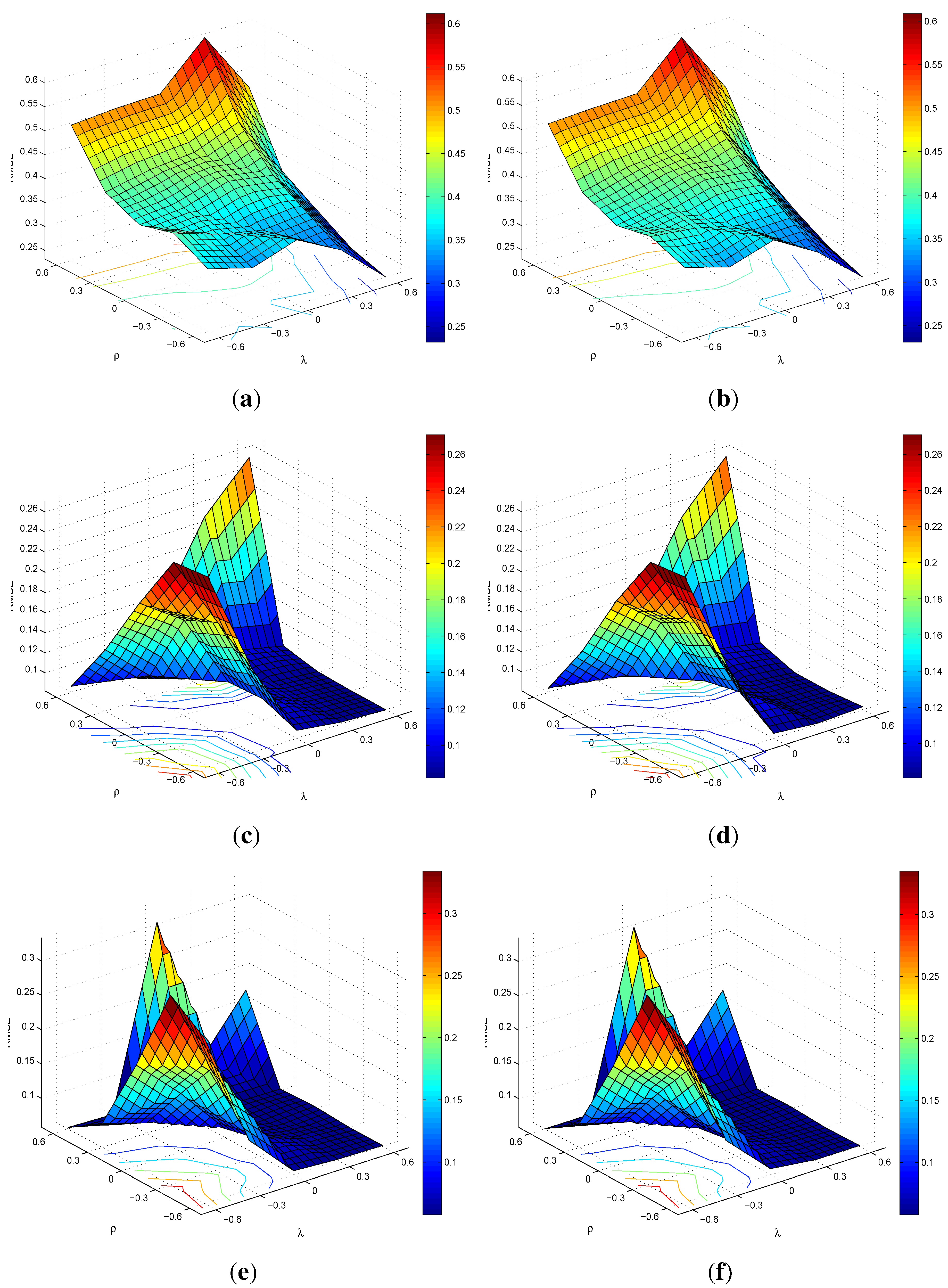
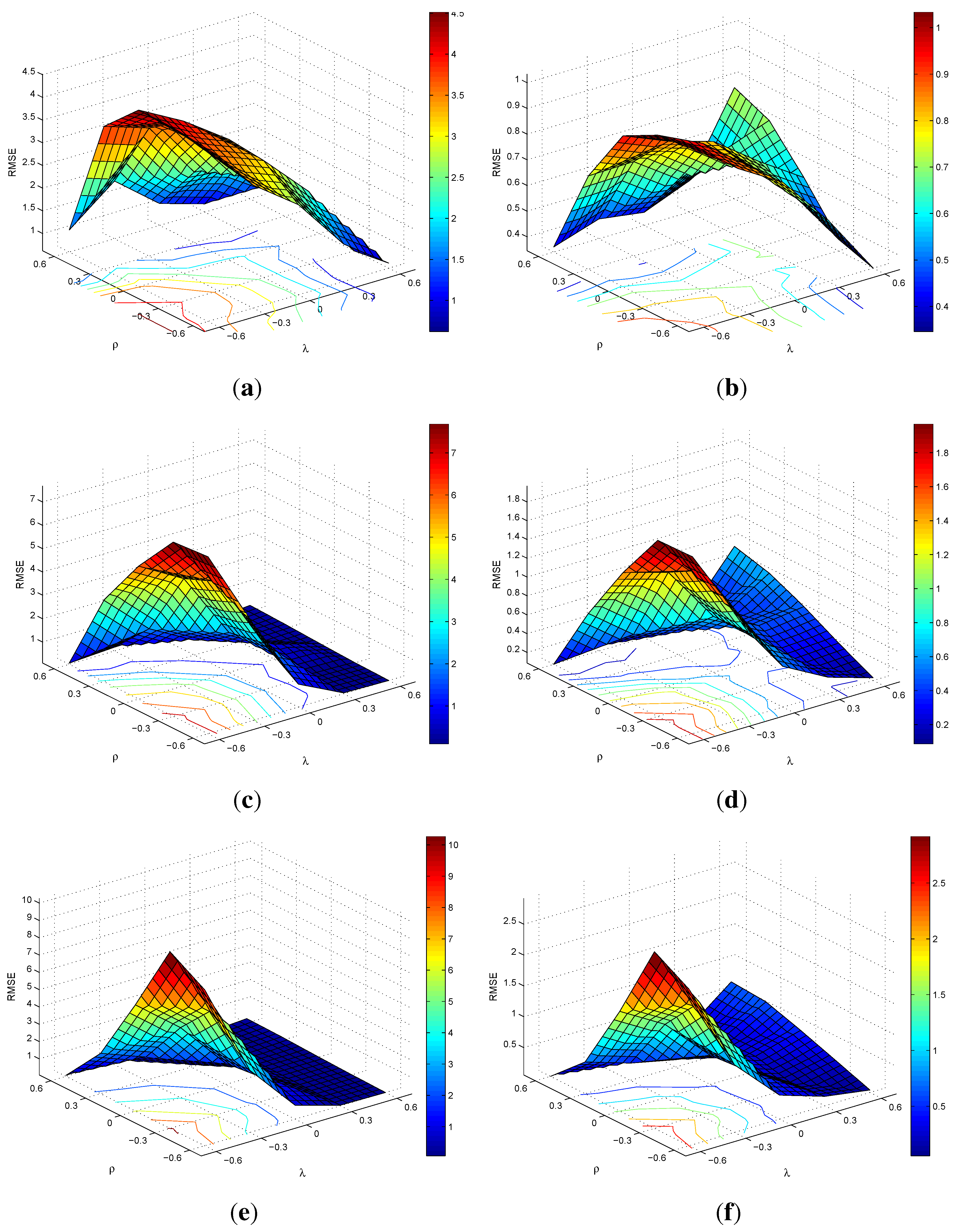
E: Surface Plots of RMSEs for SARMA(1,1)

Figure E1. RMSEs of β 1 and β 2 . (a) β 1 , n = 100 . (b) β 2 , n = 100 . (c) β 1 , n = 500 . (d) β 2 , n = 500 . (e) β 1 , n = 1,000. (f) β 2 , n = 1,000.
Econometrics 03 00101 g003
Figure E2. RMSEs of λ and ρ. (a) λ , n = 100 . (b) ρ , n = 100 . (c) λ , n = 500 . (d) ρ , n = 500 . (e) λ , n = 1,000. (f) ρ , n = 1,000.
Econometrics 03 00101 g004

Acknowledgements

I would like to thank two anonymous referees, Suleyman Taspinar, Wim Vijverberg and Gabriel Movsesyan for their helpful comments on the earlier drafts of this paper.

Conflicts of Interest

The author declare no conflict of interest.

References

  1. R.P. Haining. “The moving average model for spatial interaction.” Trans. Inst. Br. Geogr. 3 (1978): 202–225. [Google Scholar] [CrossRef]
  2. L. Anselin. Spatial Econometrics: Methods and Models. New York, NY, USA: Springer, 1988. [Google Scholar]
  3. L.W. Hepple. Bayesian and Maximum Likelihood Estimation of the Linear Model with Spatial Moving Average Disturbances. Working Papers Series; Bristol, UK: School of Geographical Sciences, University of Bristol, 2003. [Google Scholar]
  4. B. Fingleton. “A generalized method of moments estimator for a spatial model with moving average errors, with application to real estate prices.” Empir. Econ. 34 (2008): 35–37. [Google Scholar] [CrossRef]
  5. B. Fingleton. “A generalized method of moments estimator for a spatial panel model with an endogenous spatial lag and spatial moving average errors.” Spat. Econ. Anal. 3 (2008): 27–44. [Google Scholar] [CrossRef]
  6. H.H. Kelejian, and I.R. Prucha. “A generalized spatial two-stage least squares procedure for estimating a spatial autoregressive model with autoregressive disturbances.” J. Real Estate Financ. Econ. 17 (1998): 1899–1926. [Google Scholar]
  7. H.H. Kelejian, and I.R. Prucha. “A generalized moments estimator for the autoregressive parameter in a spatial model.” Int. Econ. Rev. 40 (1999): 509–533. [Google Scholar] [CrossRef]
  8. D. Das, H.H. Kelejian, and I.R. Prucha. “Small sample properties of estimators of spatial autoregressive models with autoregressive disturbances.” Pap. Reg. Sci. 82 (2003): 1–26. [Google Scholar] [CrossRef]
  9. H.H. Kelejian, and I.R. Prucha. “Specification and estimation of spatial autoregressive models with autoregressive and heteroskedastic disturbances.” J. Econom. 157 (2010): 53–67. [Google Scholar] [CrossRef] [PubMed]
  10. X. Liu, L.F. Lee, and C.R. Bollinger. “An efficient GMM estimator of spatial autoregressive models.” J. Econom. 159 (2010): 303–319. [Google Scholar] [CrossRef]
  11. L.F. Lee. “Asymptotic distributions of quasi-maximum likelihood estimators for spatial autoregressive models.” Econometrica 72 (2004): 1899–1925. [Google Scholar] [CrossRef]
  12. L.F. Lee. “GMM and 2SLS estimation of mixed regressive, spatial autoregressive models.” J. Econom. 137 (2007): 489–514. [Google Scholar] [CrossRef]
  13. L.F. Lee, and X. Liu. “Efficient GMM estimation of high order spatial autoregressive models with autoregressive disturbances.” Econom. Theory 26 (2010): 187–230. [Google Scholar] [CrossRef]
  14. J.P. Lesage. “Bayesian estimation of spatial autoregressive models.” Int. Reg. Sci. Rev. 20 (1997): 113–129. [Google Scholar] [CrossRef]
  15. J. LeSage, and R.K. Pace. Introduction to Spatial Econometrics (Statistics: A Series of Textbooks and Monographs. London, UK: Chapman and Hall/CRC, 2009. [Google Scholar]
  16. L.W. Hepple. “Bayesian techniques in spatial and network econometrics: 1. Model comparison and posterior odds.” Environ. Plan. 27 (1995): 247–469. [Google Scholar]
  17. I.R. Prucha. “Instrumental variables/method of moments estimation.” In Handbook of Regional Science. Edited by M.M. Fischer and P. Nijkamp. Berlin, Germany: Springer Berlin Heidelberg, 2014, pp. 1597–1617. [Google Scholar]
  18. L.F. Lee. “The method of elimination and substitution in the GMM estimation of mixed regressive, spatial autoregressive models.” J. Econom. 140 (2007): 155–189. [Google Scholar] [CrossRef]
  19. B.H. Baltagi, and L. Liu. “An improved generalized moments estimator for a spatial moving average error model.” Econ. Lett. 113 (2011): 282–284. [Google Scholar] [CrossRef]
  20. M. Arnold, and D. Wied. “Improved GMM estimation of the spatial autoregressive error model.” Econ. Lett. 108 (2010): 65–68. [Google Scholar] [CrossRef]
  21. D.M. Drukker, P. Egger, and I.R. Prucha. “On two-step estimation of a spatial autoregressive model with autoregressive disturbances and endogenous regressors.” Econom. Rev. 32 (2013): 686–733. [Google Scholar] [CrossRef]
  22. X. Lin, and L.F. Lee. “GMM estimation of spatial autoregressive models with unknown heteroskedasticity.” J. Econom. 157 (2010): 34–52. [Google Scholar] [CrossRef]
  23. H.H. Kelejian, and D. Robinson. “A suggested method of estimation for spatial interdependent models with autocorrelated errors, and an application to a county expenditure model.” Pap. Reg. Sci. 72 (1993): 297–312. [Google Scholar] [CrossRef]
  24. J. Besag. “Spatial interaction and the statistical analysis of lattice systems.” J. R. Stat. Soc. Ser. B (Methodological) 36 (1974): 192–236. [Google Scholar]
  25. S. Richardson, C. Guihenneuc, and V. Lasserre. “Spatial linear models with autocorrelated error structure.” J. R. Stat. Soc. Ser. D (The Statistician) 41 (1992): 539–557. [Google Scholar] [CrossRef]
  26. L.W. Hepple. “Bayesian techniques in spatial and network econometrics: 2. Computational methods and algorithms.” Environ. Plan. 27 (1995): 615–644. [Google Scholar]
  27. B.D. Ripley. Spatial Statistics. Wiley Series in Probability and Statistics; Hoboken, New Jersey, USA: John Wiley & Sons, 2005. [Google Scholar]
  28. R. Haining. “Trend-Surface models with regional and local scales of variation with an application to aerial survey data.” Technometrics 29 (1987): 461–469. [Google Scholar]
  29. K.V. Mardia, and R.J. Marshall. “Maximum likelihood estimation of models for residual covariance in spatial regression.” Biometrika 71 (1984): 135–146. [Google Scholar] [CrossRef]
  30. L.W. Hepple. “A Maximum likelihood model for econometric estimation with spatial series.” In Theory and Practice in Regional Science. Edited by I. Masser. London papers in regional science 6; London, UK: Pion Limited, 1976. [Google Scholar]
  31. K.M. Abadir, and J.R. Magnus. Matrix Algebra. Econometric Exercises; New York, NY, USA: Cambridge University Press, 2005. [Google Scholar]
  32. L.F. Lee. “Identification and estimation of econometric models with group interactions, contextual factors and fixed effects.” J. Econom. 140 (2007): 333–374. [Google Scholar] [CrossRef]
  33. L.F. Lee, X. Liu, and X. Lin. “Specification and estimation of social interaction models with network structures.” Econom. J. 13 (2010): 145–176. [Google Scholar] [CrossRef]
  34. H.H. Kelejian, and I.R. Prucha. Specification and Estimation of Spatial Autoregressive Models with Autoregressive and Heteroskedastic Disturbances. College Park, MD, USA: Department of Economics, University of Maryland, 2007. [Google Scholar]
  35. R.K. Pace, J.P. LeSage, and S. Zhu. Spatial Dependence in Regressors and Its Effect on Performance of Likelihood-Based and Instrumental Variable Estimators, 30th Anniversary ed. Advances in Econometrics; Bingley, UK: Emerald Group Publishing Limited, 2012, Volume 30, pp. 257–295. [Google Scholar]
  36. O. Dogan, and T. Suleyman. GMM Estimation of Spatial Autoregressive Models with Autoregressive and Heteroskedastic Disturbances. Working Papers 001; New York, NY, USA: City University of New York Graduate Center, Ph.D. Program in Economics, 2013. [Google Scholar]
  • 1Fingleton [4] and Baltagi and Liu [19] do not compare the finite sample efficiency of their estimators with the MLE.
  • 2See Kelejian and Prucha [9].
  • 3For a definition and some properties of uniform boundedness, see Kelejian and Prucha [9].
  • 4There are some other formulations for the parameter spaces in the literature. For details, see Kelejian and Prucha [9] and LeSage and Pace [15]. Note that the parameter spaces for β 0 and σ 0 2 are not required to be compact. As shown in Equations (8a) and (8b), the MLE of these parameters is an OLS-type estimator; hence, boundedness is enough for the parameter spaces.
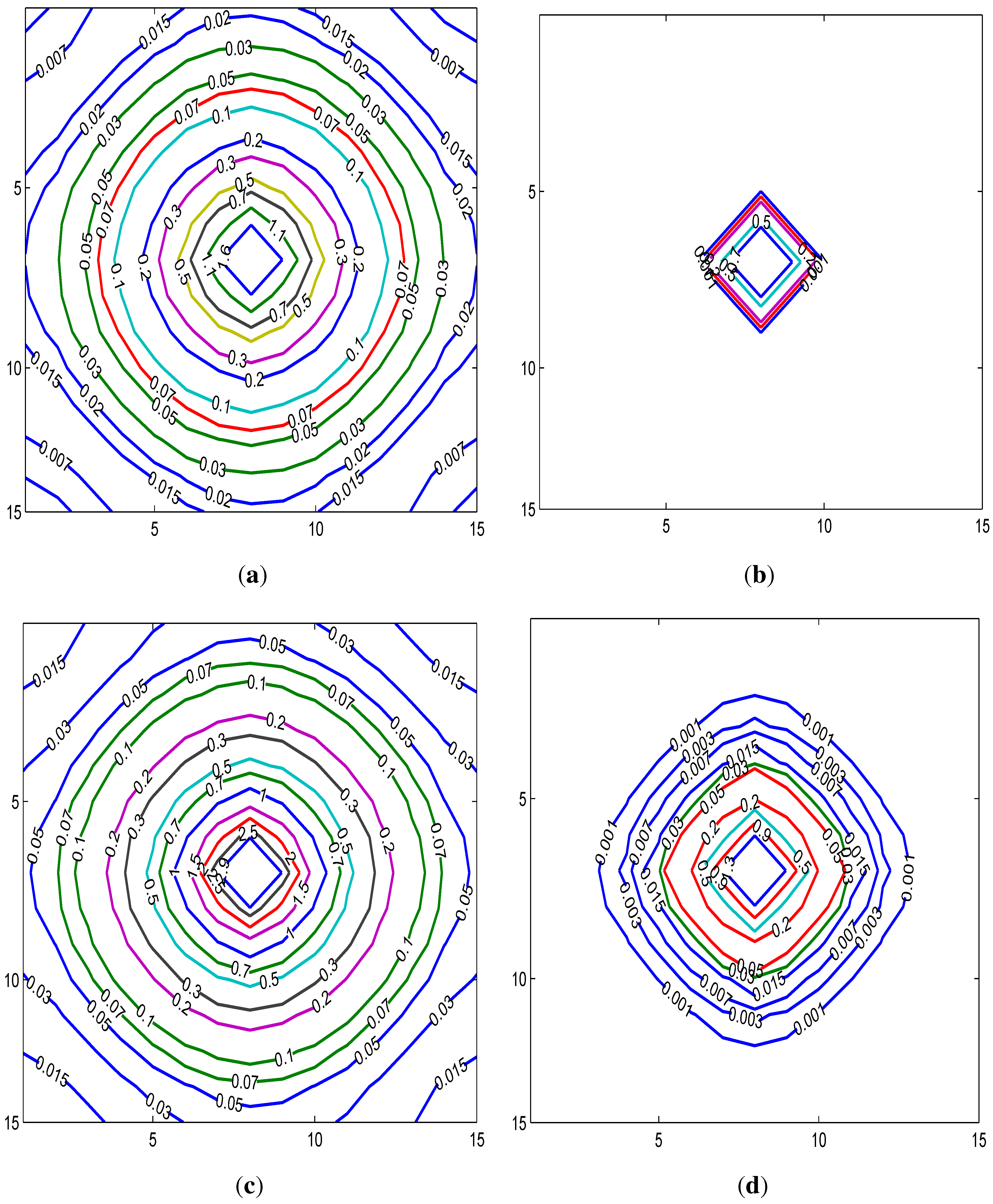
  • 5For easy comparison, we set λ 0 = 0 . 9 for SAR, ρ 0 = - 0 . 9 for SMA, ( λ 0 , ρ 0 ) = ( 0 . 5 , 0 . 9 ) for SARAR(1,1) and ( λ 0 , ρ 0 ) = ( 0 . 5 , - 0 . 9 ) for SARMA(1,1). The disturbance of the unit located at the center of the lattice is increased by three.
  • 6 d i j = R 0 × arccos cos | l o n g i t u d e i - l o n g i t u d e j | cos ( l a t i t u d e i ) cos ( l a t i t u d e j ) + sin ( l a t i t u d e i ) sin ( l a t i t u d e j ) , where R 0 is the Earth’s radius.
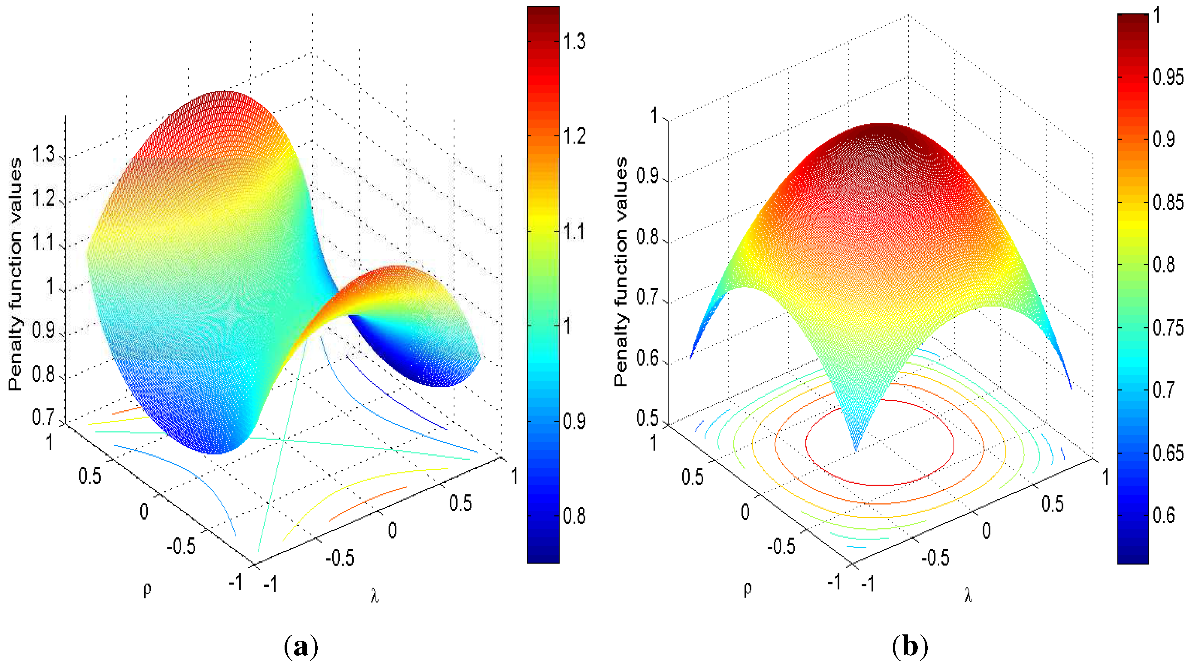
  • 7For SARAR(1,1), the penalty function is f ( λ , ρ , W n , M n ) = | S n ( λ ) | 2 n | R n ( ρ ) | 2 n .
  • 8For these results, I use the derivative rule given by ln | R n ( ρ ) | ρ = tr R n - 1 ( ρ ) × R n ( ρ ) ρ . For a proof, see (Abadir and Magnus [31], p. 372). Also note the commutative property of R n - 1 ( ρ ) M n = M n R n - 1 ( ρ ) = H n ( ρ ) .
  • 9Here, Diag B 1 , , B G denotes the block diagonal matrix in which the diagonal blocks are m i × m i matrices of B i s.
  • 10Note that 1 n t r ( G ¯ n - G n ) = 0 .

