Article

Bayesian Inference for Latent Factor Copulas and Application to Financial Risk Forecasting

by
Benedikt Schamberger
,
Lutz F. Gruber
and
Claudia Czado
*
Department of Mathematics, Technical University of Munich, 85748 Garching, Germany
*
Author to whom correspondence should be addressed.
These authors contributed equally to this work.
Econometrics 2017, 5(2), 21; https://doi.org/10.3390/econometrics5020021
Submission received: 25 November 2016 / Revised: 26 April 2017 / Accepted: 8 May 2017 / Published: 23 May 2017
(This article belongs to the Special Issue Recent Developments in Copula Models)

Abstract

:
Factor modeling is a popular strategy to induce sparsity in multivariate models as they scale to higher dimensions. We develop Bayesian inference for a recently proposed latent factor copula model, which utilizes a pair copula construction to couple the variables with the latent factor. We use adaptive rejection Metropolis sampling (ARMS) within Gibbs sampling for posterior simulation: Gibbs sampling enables application to Bayesian problems, while ARMS is an adaptive strategy that replaces traditional Metropolis-Hastings updates, which typically require careful tuning. Our simulation study shows favorable performance of our proposed approach both in terms of sampling efficiency and accuracy. We provide an extensive application example using historical data on European financial stocks that forecasts portfolio Value at Risk (VaR) and Expected Shortfall (ES).

1. Introduction

Copulas (Sklar 1959) are powerful models of multivariate dependence. Copula modeling has had profound impact on the field of financial econometrics by substantially improving the quality of key metrics of financial risk of portfolios such as Value at Risk (VaR) and Expected Shortfall (ES) (see Embrechts et al. (1999)).
Even in the simplest multivariate Gaussian model the number of correlation parameters increases quadratically in the number of variables d, and the quadratic growth in dependence parameters also extends to more general copula models. This illustrates that sparse modeling of multivariate dependence becomes critical for robust estimation and forecasting in increasingly high-dimensional problems. One approach to achieve parsimony is to use dynamic latent factors to capture dependence induced by common underlying economic activity components. Dynamic factor models, also known as index models, were first suggested by Geweke (1978) and Sargent and Sims (1977) based on ideas of Burns and Mitchell (1946), and later generalized by Forni et al. (2000, 2012), among others. Factor modeling has become popular in credit risk modeling (see for example Gordy (2000); Crouhy et al. (2000)), with the multivariate Gaussian and t copulas serving as the backbone of many credit risk models (Frey and McNeil 2003).
We present a Bayesian latent factor copula model that reduces the quadratic growth rate of the number of parameters to a linear one. Factor copulas have previously been successfully employed to scale the dimension of multivariate dependence models (Murray et al. (2013); Krupskii and Joe (2013, 2015); Oh and Patton (2017)). The pair copula construction-based factor model includes the Gaussian factor model as a special case, and allows much more flexible fine-tuning to capture elaborate dependence characteristics than Murray et al. (2013) and Oh and Patton (2017)’s factor copula models.
Our proposed model builds on Krupskii and Joe (2013)’s, and shares their strategy to use bivariate pair copulas to couple the marginal variables with a latent factor. In contrast to their work, we present a Bayesian learning strategy that replaces frequentist uniform integration over the latent factor with Bayesian posterior simulation. A key advantage of Bayesian modeling over frequentist modeling is that credible intervals of the predictive distributions of derived quantities such as value at risk or expected shortfall can be easily obtained.
Copula models are typically estimated in two stages (see, for example, (Joe and Xu 1996) and (Joe 2005)): first, univariate marginal models are estimated to make the observed data independent and identically distributed on each of the margins by applying the cumulative distribution function of the marginal models to the observed data; second, a (multivariate) copula is estimated based on the transformed, marginally i.i.d. input data. The generally unfavorable view of two stage estimation procedures must be suspended in the context of copula estimation: the definition a copula requires that the marginal distributions of a copula be uniform on the unit interval; hence marginal models must be estimated to obtain said marginally i.i.d. uniform data before any copula modeling can be performed. Indeed, Czado et al. (2011)’s study confirms that joint Bayesian estimation of the marginal models and copula does not lead to improved estimates; the Markov chain Monte Carlo (MCMC) iterations until convergence of the marginal models produce non-uniform marginal input data for the copula, which leads to substantially increased MCMC runtime. An added benefit of estimating the marginal and dependence models separately is that inference methods for the copula can be applied universally as they do not depend on characteristics of the marginal data (which is marginally i.i.d. uniform, by definition).
We use adaptive rejection Metropolis sampling (ARMS) within Gibbs sampling (Gilks et al. 1995) for posterior simulation to eliminate the need for lengthy pilot runs to fine-tune proposal parameters: this strategy retains the Gibbs sampler’s main conceptual idea to recursively simulate from the full conditional distributions, but uses ARMS to generate samples from full conditionals that cannot be drawn from directly. This way, there is no need for Metropolis-Hastings updates (Metropolis et al. (1953); Hastings (1970)), which typically require substantial effort from the user to carefully tune the proposals.
The proposed approach is then illustrated to forecast the VaR and ES of a portfolio of European bank stocks. The Bayesian factor copula model combines univariate daily one-day ahead from the marginal return time series, which are modeled by dynamic linear models (DLMs) with ARMA(1,1) structure (West and Harrison 1997).
The paper is organized as follows: we define the latent factor copula in Section 2, and present Bayesian theory as well as several MCMC-based strategies for posterior simulation in Section 3. Section 4 presents a simulation study that investigates the sampling performance of our simulation strategies, and Section 5 discusses an application to financial time series data. The paper concludes with summary comments in Section 6.

2. Latent Factor Copulas

A latent factor copula models the dependence among d variables u j U n i f ( 0,1 ) , j = 1 : d , by a linking copula c j ( u j , v ; θ j ) with copula parameter θ j for each variable u j and one common latent variable v. Each of the linking copulas c j can be any bivariate copula; a detailed discussion of many bivariate copulas can be found in Joe (1997). Conditionally on the latent variable v, the density function of the latent factor copula is
c ( u 1 , , u d | v ) = j = 1 : d c j ( u j , v ; θ j ) .

Linking Copulas

We will use the bivariate Gaussian and Gumbel copulas (Joe 1997) as candidate linking copulas; these are the same linking copulas used by Krupskii and Joe (2013). The Gaussian copula is tail-independent and symmetric, while the Gumbel copula is asymmetric and lower tail-dependent. Density functions and properties about these copulas are summarized in Table 1, while Table 2 shows pairs plots for several different parameter values. To further reduce model complexity, we assume a common linking copula family for all margins, but allow for a margin-specific copula parameter, that is, c j ( u j , ν , θ j ) = c ( u j , ν , θ j ) .
We parameterize the linking copulas by the Fisher z-transformation of Kendall’s τ , given by
z = z ( τ ) = 1 2 ln 1 + τ 1 τ , τ ( 1 , 1 ) ,
τ = z 1 ( z ) = 1 2 e 2 z + 1 , z R .
This is a more convenient parameterization for analysis across different copula families than the copulas’ natural parameters, because it makes the parameters comparable across different copula families. The domains of the Fisher z-transformation depend on the copula family; for example, the Fisher z parameter of a Gumbel copula takes values in ( 0 , ) , while that of the Gaussian copulas takes values in ( , ) .

Likelihood

Let u = ( u t j ) t = 1 : T , j = 1 : d be T i.i.d. d-dimensional observations u t = ( u t 1 , , u t d ) , t = 1 : T , in the copula domain [ 0,1 ] d ; and denote the states of the latent factor by v = ( v t ) t = 1 : T . The joint likelihood function ( θ , v ; u ) of the latent factor v and copula parameters θ = ( θ j ) j = 1 : d follows from (1) as
( θ , v ; u ) = t = 1 : T j = 1 : d c j ( u t j , v t ; θ j ) .
Substituting the Fisher z parameters z = ( z 1 , , z d ) , where z i : = z ( h j ( θ j ) (see (2) for z ( · ) and Table 1 for h ( · ) ), for the natural copula parameters θ , the joint likelihood of the latent factor v and Fisher z parameters z = ( z j ) j = 1 : d follows as
( z , v ; u ) = t = 1 : T j = 1 : d c j u t j , v t ; h j 1 z 1 ( z j ) .

Frequentist Inference

Frequentist inference (Krupskii and Joe 2013) integrates over the latent variable v to obtain the unconditional density function of the latent factor copulas as
c ( u 1 , , u d ) = 0 1 j = 1 : d c j ( u j , v ; θ j ) d v ,
and then maximizes the unconditional likelihood function with respect to the copula parameters.

3. Bayesian Posterior Analysis

In Bayesian analyses, prior information about the unknown parameters is quantified in a “prior distribution.” Once data is observed, the prior distribution and likelihood are combined to derive the posterior distribution—the distribution of the unknown parameters given the observed data. As the posterior distribution typically can not be derived in a closed form, Markov chain Monte Carlo (MCMC) methods are used to simulate from the posterior distribution.

3.1. Prior Distributions

Prior for Copula Parameters z

Each linking copula’s Fisher z parameter can take values in D SG = D G = ( 0 , ) or D N = ( , ) , depending on whether it is a Gaussian or Gumbel copula. We propose normally-distributed priors on the Fisher z parameter, truncated to the allowable parameter range D SG = D G and D N , respectively. Furthermore, we assume that the priors are independent over all linking copulas j = 1 : d :
z j N D j ( 0 , σ j 2 ) , π ( z ) = j = 1 : d n D j ( z j ; 0 , σ j 2 ) ,
where N D ( μ , σ 2 ) denotes a normal distribution with mean μ and variance σ 2 truncated to D with corresponding probability density function n D ( · ; μ , σ 2 ) .

Prior for Latent Factor v

In line with the frequentist assumption that integrates out the latent factor v using a uniform density, we choose a uniform prior for v , independent across observations t = 1 : T ,
v t U n i f ( 0 , 1 ) , π ( v ) = t = 1 : T π ( v t ) 1 .
Given that the latent factor v t feeds directly into a copula distribution, the uniform distribution on the unit interval is the only natural choice that does not violate the requirement of uniform copula margins.

Joint Prior for z and v

We assume no dependence between the latent factor v and copula parameters z , and choose the joint prior density π ( z , v ) of z and v as the product of the individual prior densities,
π ( z , v ) = π ( z ) π ( v ) .
Independence priors are a common choice in Bayesian modeling, and they do not prevent the posterior from exhibiting data-induced dependence; more comments below after the posterior density (10).

3.2. Posterior Distribution and Full Conditionals

Posterior Density

An analytical expression of the joint posterior density p ( z , v | u ) of the copula parameters z and latent factor v , given observations u can only be obtained up to a normalizing constant,
p ( z , v | u ) ( z , v ; u ) π ( z , v ) .
Indeed, this posterior density cannot be factorized into independent marginal distributions for z and v , given that the likelihood function does not exhibit such a product form and thus induces multivariate dependencies in the posterior distribution.

Full Conditionals

The full conditionals of the latent factor v = ( v t ) t = 1 : T and Fisher z parameters z = ( z j ) j = 1 : d can be derived by straightforward calculation.
The joint posterior density p ( z , v | u ) of z and v , given observations u can be written as
p ( z , v | u ) ( z , v ; u ) π ( z , v ) = ( z , v ; u ) π ( z ) π ( v ) = ( z , v ; u ) j = 1 : d N D j ( z j ) = t = 1 : T j = 1 : d c j u t j , v t ; h j 1 z 1 ( z j ) j = 1 : d n D j ( z j ; 0 , σ j 2 ) ;
here we used the likelihood from (5) and priors from (7) to (9). Then, for all t = 1 : T , the full conditional of v t , given all other latent factor states v t : = ( v 1 , , v t 1 , v t + 1 , , v T ) , observations u and Fisher z copula parameters z is
p ( v t | v t , u , z ) = p ( z , v | u ) p ( z , v t | u ) p ( z , v | u ) j = 1 : d c j ( u t j , v t ; z j ) ,
where the prior densities of v t and z are constant factors independent of v t .
Similarly to (12), the full conditional of z l , given all other Fisher z copula parameters z j , observations u and latent factor v , can be derived as
p ( z j | z j , u , v ) t = 1 : T c j ( u t j , v t ; z j ) n D j ( z j ; 0 , σ j 2 ) .

3.3. MCMC Methods for Posterior Simulation

The complex forms of the posterior and full conditional densities render direct sampling infeasible. We investigate the performance characteristics of several different sampling strategies:
  • Metropolis-Hastings within Gibbs sampling (Metropolis et al. (1953); Hastings (1970); Gelfand and Smith (1990)):
    -
    MCM: Truncated normal proposals for z and Beta proposals for v ; proposal mode and curvature match those of the full conditionals;
    -
    EVM: Gamma proposals for z and Beta proposals for v ; proposal expectation and variance match those of the full conditionals;
    -
    IRW: Truncated normal random walk proposals for z and uniform independence proposals v ; and
  • ARMGS: Adaptive rejection Metropolis sampling within Gibbs sampling (Gelfand and Smith (1990); Gilks et al. (1995)).
Details of the sampling schemes are given in Appendix A.1. We will investigate these strategies in a simulation study using Gumbel linking copulas (Section 4), and then adapt the best-performing method to also work for Gaussian linking copulas. Here the main difference will be the extension from only non-negative Fisher z values to positive and negative values.

4. Simulation Study

We test our four different MCMC sampling strategies in strong, weak, and mixed dependence scenarios. The goal is to verify that these samplers provide good estimates, and to determine if some perform better than others.

4.1. Simulation Setup

Scenarios

To explore the behavior of the Gibbs sampler under different dependence characteristics between the marginal data u and the latent factor v , we consider three different scenarios: in the first scenario, all linking copulas show weak dependence, with Kendall’s τ values of 0.1 τ 0.2 ; in the second scenario, we use high Kendall’s τ values of 0.5 τ 0.8 ; and in the third scenario, we use a combination of strong and weak dependence between the marginal data and latent factor with Kendall’s τ ’s of the linking copulas varying between 0.1 τ 0.8 . Table 3 summarizes the Kendall’s τ ’s, copula parameters θ , and Fisher z parameters z of all scenarios.

Simulation Data

We investigate N = 100 data sets from the latent factor copula model in three different scenarios. Each simulation data set contains T = 200 observations of dimension d = 5 . We use Gumbel linking copulas for each pair c 1 , , c 5 . As an asymmetric extreme value copula with upper tail dependence and lower tail independence, the bivariate Gumbel copula can be a good fit to model financial data such as large negative stock returns: the probability of many stocks selling off simultaneously tends to be much higher than the probability of many stocks all making outsize gains on the same day. The density of the bivariate Gumbel copula quickly tends to infinity for ( u , u ) ( 0,0 ) or ( u , u ) ( 1,1 ) , allowing to test the robustness of our proposed sampling routines for linking copulas that show difficult numerical behavior.

Posterior Simulation

For each of the N = 100 simulation data sets from the three scenarios described in Section 4.1, we generated 10,000 MCMC samples with each sampling method from Section 3.3, using the starting values from our heuristic of Appendix A.2 and prior variances σ j 2 = 100 2 for the Fisher z copula parameters.
The proposal variance for our IRW method were tuned in pilot runs with 1,000 iterations each to achieve acceptance rates between 20% and 30% for each Fisher z parameter z 1 , , z 5 ; we specified this range of desirous acceptance rates in line with Roberts et al. (1997)’s suggestion for tuning to 23%. Uniform U n i f ( 0,1 ) proposals for the latent factor v = ( v 1 , , v T ) lead to acceptance rates around 20%, which we accepted as good enough. These settings performed well across all three scenarios.

4.2. Results

Kendall’s τ Pair Copula Parameters

For ease of interpretation, we analyze the results posterior samples in terms of Kendall’s τ , which is a simple transformation from Fisher’s z. Posterior trace plots show immediate convergence to an equilibrium state as well as good mixing behavior (see Figure 1); the latter is confirmed by posterior density plots. The runtimes of our different sampling strategies varied substantially: the slowest method (EVM) took 14 times as long as the fastest (IRW) to generate 10,000 posterior samples (Table 4); the faster methods, IRW and ARMGS, also out-performed the slower ones in terms of effective sample size (ESS; Thiébaux and Zwiers (1984)) per minute. Table 4 shows that Metropolis-Hastings within Gibbs sampling with IRW updates was marginally faster than adaptive rejection Metropolis sampling within Gibbs sampling (ARMGS), but the latter’s coverage of credible intervals was better. Metropolis-Hastings within Gibbs Sampling with MCM updates provided the smallest point estimation errors (both mean absolute deviation and mean squared errors) of all analyzed Bayesian procedures, but it still trails frequentist maximum likelihood estimation (MLE). Overall, our ARMGS and IRW performed substantially better than MCM and EVM. As an adaptive procedure, ARMGS requires less effort of the user than IRW, making it the grand winner.

Latent Factor States

Bayesian inference of our latent factor copula also provides posterior samples of the latent factor v , which can enable a more thorough analysis of dependence patterns in real-world applications. Again, adaptive rejection Metropolis sampling within Gibbs sampling (ARMGS) is the grand winner, showing the best combination of sampling efficiency (ESS/min), coverage of credible intervals and accuracy of point estimates (Table 5). The MCM and EVM methods produced very slightly better point estimates that ARMGS and IRW, but the latter two methods realized a more than 10 times higher effective sample size during the benchmark 10 min runtime than MCM and EVM.

5. Application: Portfolio Value at Risk of European Financial Stocks

This section presents a case study to forecast value at risk (VaR) and expected shortfall (ES) using a dynamic multivariate model that consists of our latent factor copula and univariate time series DLMs. We analyze the daily log-returns of eight European bank stocks that are head-quartered in euro zone countries over a ten year period from January 2004 through December 2013. We use adjusted closing prices, which correct for dividends, (reverse) stock splits, and other measures to calculate the daily log-returns (data are downloaded from http://finance.yahoo.com). Table 6 lists details of the selected stocks, including their ticker symbols, which we will use to identify stocks in this section, as well as the exchange they are traded on.
Since the data set includes stocks from several European countries, trading days may differ due to varying bank holidays for each exchange. Therefore, we use the union of all trading days, where for stocks that are not traded at a given day, the asset value of the previous day is reused. This method introduces some additional zero returns into the data, but avoids altering actual historical returns which would happen if we intersected the trading days of different exchanges. The so expanded data set consists of 2,606 daily 8-dimensional log-returns.

5.1. Marginal Analysis

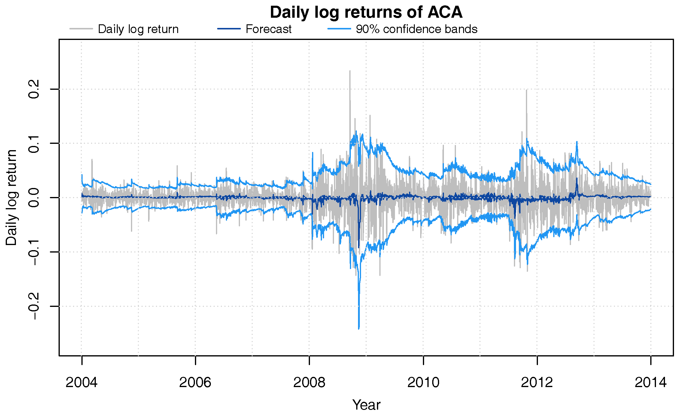
Figure 2 shows the daily log-returns of Credit Agricole (ACA); the historical returns of the other stocks look very similar. The initial period from 2004 through 2007 was relatively calm, and was followed by a more turbulent period beginning in 2008. Market nervousness intensified during the second half of 2008, when, at the height of the sub-prime mortgage crisis, Lehman Brothers collapsed. Volatility receded in the second half of 2009 and remained subdued until the second half of 2011, when the European debt crisis hit the markets. Volatility remained at elevated levels through 2012, and then showed a gradual decline in 2013.

Time Series DLMs

Since we are interested in online learning and forecasting of the return time series, we use the dynamic linear model (DLM), which is also a model of dynamic stochastic volatility. While the economics literature tends to favor GARCH models to model financial time series data, we view the DLM as a better choice as it allows for fast and efficient fully Bayesian online learning and forecasting based on analytical expressions of the posterior and predictive distributions, which can be evaluated in fractions of a second, and can also model stochastic, time-varying volatilities. If we were using GARCH models, we would have to perform lengthy MCMC-based posterior simulation for each trading day t in our dataset to generate sequential out-of-sample predictions; this computational disadvantage disqualifies GARCH models from further consideration in our study.
We use an ARMA(1,1)-structure in our marginal time series DLM with beta discounting for on-line learning of stochastic observational variances (West and Harrison 1997). Denote the daily log-returns of the j-th series by ( y j t ) t = 1 : T ; the model is defined by observation Equation (14)
y j t = μ j t + ϕ j t y j , t 1 + ψ j t ϵ j , t 1 + ϵ j t = : F j t θ j t + ϵ j t ,
which relates the observations y j t to a time-varying local level μ j t , ARMA(1,1)-structure with dynamic regression coefficients ϕ j t and ψ j t , and conditionally normally-distributed observation error ϵ j t N ( 0,1 / λ j t ) ; the predictors F j t = ( 1 , y j , t 1 , ϵ j , t 1 ) are just those of a regular local-level ARMA(1,1) model.
Appendix C summarizes the analytic filtering equations to sequentially learn the model, and elaborates on the system equations for the prior evolutions of the states θ j t = ( μ j t , ϕ j t , ψ j t ) and observational precision λ j t > 0 (see Equations (A8) and (A10)).

Results

We started the analysis with initial normal-gamma priors as follows:
( θ j 1 , λ j 1 ) | D 0 N G ( a j 1 , R j 1 , r j 1 , c j 1 ) ,
where a j 1 = ( 0 , 0 , 0 ) , R j 1 = 10 3 · I 3 , r j 1 = 5 and c j 1 = 10 3 , and the N G notation is as explained in Appendix C. For forward filtering, we used the discount factors β = 0.97 and δ = 0.99 ; these values provide a desirable balance between robustness of forecasts and rate of adaption to market movements, and are similar to those used in existing literature (e.g., Gruber and West 2016).
Figure 2 shows the DLM’s sequential out-of-sample trend forecasts and confidence bands for ACA. It can be seen that the one-day ahead forecasts quickly adapt to changes in the volatility of the underlying stock. Table 7 shows that with our choice of discount factors, the coverage of the obtained forecast confidence intervals are very close to their theoretical values.
Copula data is obtained by transforming the observed log-returns y j t using the cumulative distribution function of the one-day ahead forecast t-distribution of y j t given information set D t 1 (see Equation (A4) of Appendix C). The forecast t-distribution already accounts for uncertainty of the model parameters; it is obtained by integrating out the parameters of the normal innovation/residual distribution weighted by their respective step ahead prior distributions. The so transformed data lie in the unit interval ( 0,1 ) , and we will denote it by u j t . We use the observations from 2004 as an initial learning data set and ignore them in further analyses; the 2,345 remaining 8-dimensional transformed observations ( u j t ) define our copula data set.

5.2. Bayesian Latent Factor Copula Analysis

We used the adaptive rejection Metropolis Gibbs sampler introduced in Section 3.3 for Bayesian posterior simulation of the parameters and latent factors of our copula model. We partitioned the resulting copula data ( u j t ) by calendar year (each year consists of roughly 260 daily observations), and select a separate copula model for each year. These annually updated models allow proper out-of-sample analysis, which would not be possible if we had estimated the model using the entire data set.
For each of the nine years, we considered three different linking copulas: the Gaussian, Gumbel and survival Gumbel copulas. We simulated 11,000 posterior samples for each year and choice of bivariate linking copulas. We chose the starting values as discussed in Appendix A.2, and discarded the first 1,000 of MCMC iterations as burn-in, resulting in a posterior sample size of 10,000 .
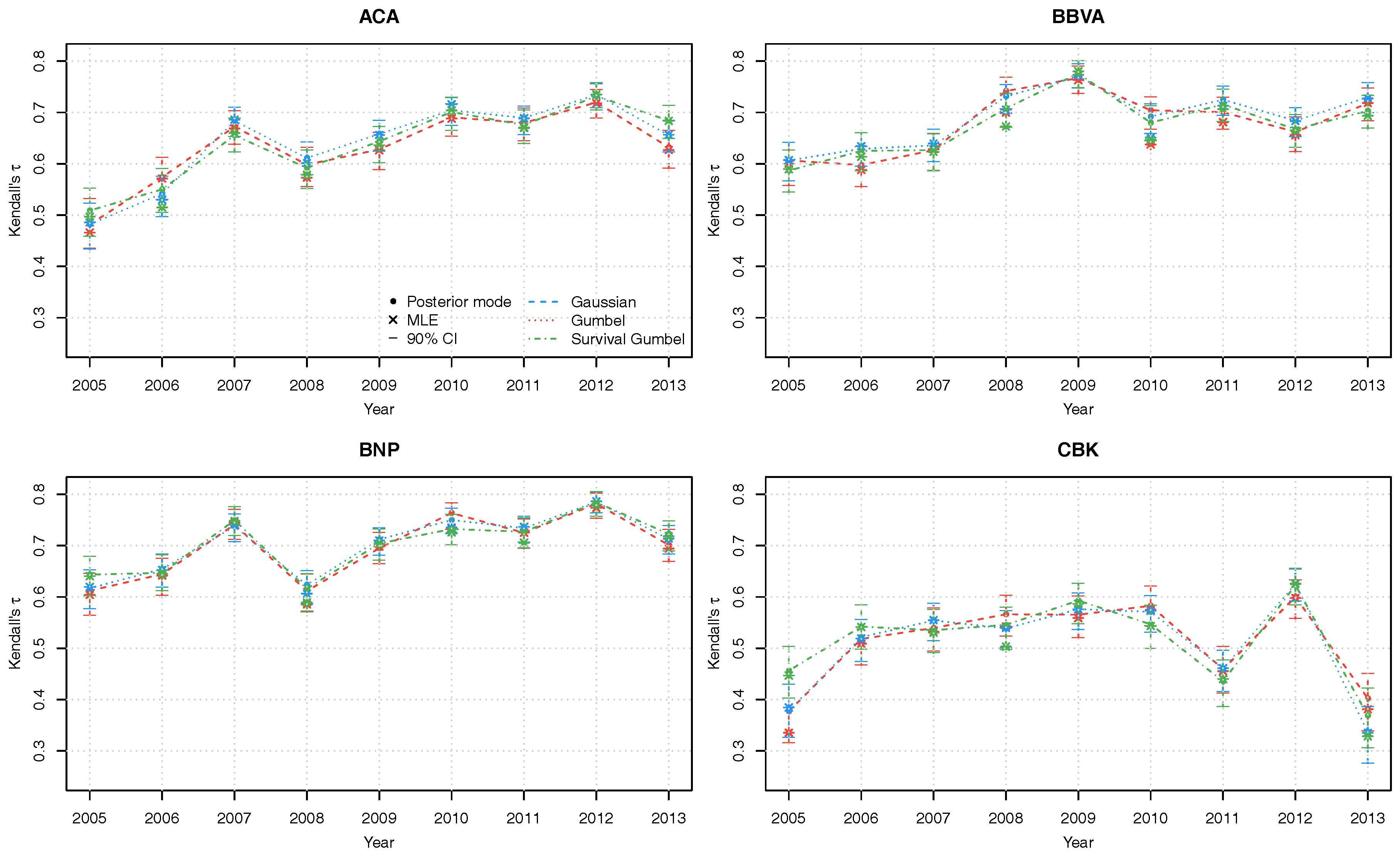
The Kendall’s τ dependence parameters between each series j = 1:8 and the latent factor v are solidly positive, taking values between 0.3 and 0.8 . Furthermore, there is substantial variation of the dependence parameters over the years (Figure 3). The posterior mode estimates for the three linking copulas are generally similar, with slight differences noticeably only in the details. We stress again that the credible intervals obtained through Bayesian posterior simulation allow for quantification of estimation uncertainty, which is not available in frequentist analysis.
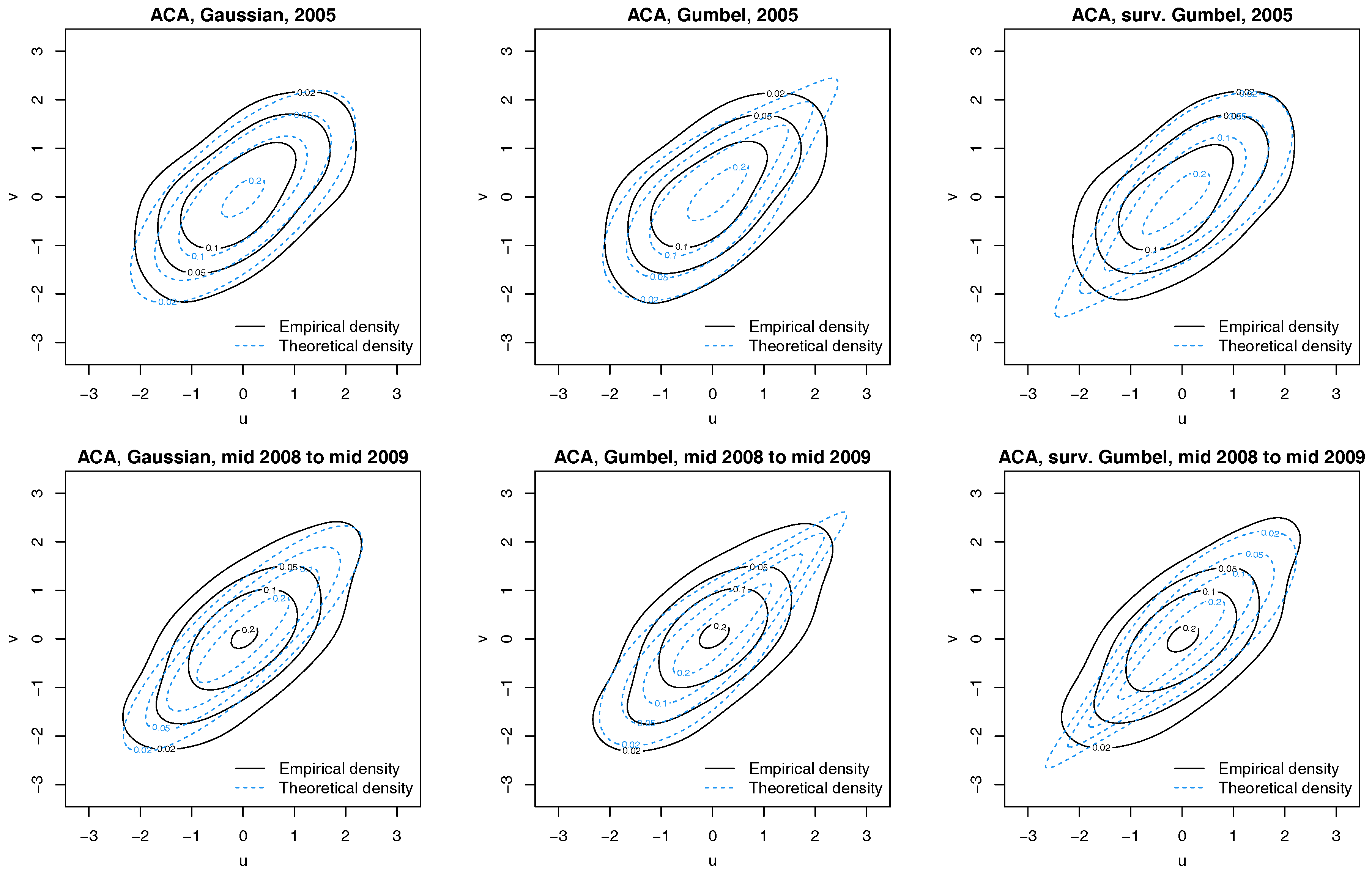
Next, we verify our implicit assumption that the bivariate distribution of every series’ copula data and the latent factor v is the one of the selected linking copula. Figure 4 shows normalized contour plots of the filtered Credit Agricole (ACA) and latent factor pairs ( u ACA , t , v ^ t ) for all three linking copulas; here we estimated each latent factor state v t by its sample posterior mean across all 10,000 MCMC iterations. The theoretical contours of the densities of the linking copulas (with posterior mean parameter) are provided for context. A visual inspection of Figure 4 reveals that the data are best modeled by a Gaussian linking copula, given that the data lack asymmetries so typical for the (survival) Gumbel copula.

5.3. Value at Risk and Expected Shortfall Forecasts

Value at risk (VaR) is one of the most widely used metrics to measure risk of financial assets. Furthermore, many current industry regulations such as Basel II/III (Basel Committee on Banking Supervision 2006, 2011) and Solvency II (European Parliament and Council 2009) use VaR to measure the risk exposure of banks and insurance companies. In recognition of the importance of VaR in real-world applications, we provide a blueprint for implementation as well as rigorous statistical verification of our model’s forecasting performance.
Expected shortfall (ES) is a risk measure that is based on VaR, and is slated to replace VaR as the prime risk measure imposed by regulators (see, for example, Basel Committee on Banking Supervision (2013)). In contrast to VaR, ES is a coherent risk measure, and a worst-case value can be derived by using the comonotonic copula (McNeil et al. 2005, Remark 6.17.). However, ES is only defined for random variables with a finite mean, which might be problematic when modeling operational losses or the losses resulting from natural catastrophes.

Forecasting Method

As in Section 5.2, we estimated the copula dependence model using data from the previous year so that the forecasts for the current year are obtained out-of-sample; for example, we learned the copula using data from 2005, and used this copula without any further adjustments to generate forecasts for each trading day in 2006. We combine the yearly changing copula with the daily updated DLMs to obtain up-to-date forecasts for each trading day. Our DLM-filtered copula data cover the years 2005 to 2013, so the resulting forecasts were for 2006 to 2014. For each day, we drew 1,000 samples from that year’s copula, and transformed the ( 0,1 ) -copula data to the observation scale using the sequential step-ahead forecast t-distributions of the marginal time series DLMs.
We used a family-restricted regular vine copula ( R V R ) as a benchmark model to test our latent factor copula against. We allowed the pair copula families to be Gaussian, Student’s t, (survival) Gumbel, Frank or BB1; these copulas can describe tail-dependent and tail-independent, and symmetric and asymmetric dependence characteristics. The tree structure and pair copula families were selected using Dißmann et al. (2013)’s selection strategy as implemented in Schepsmeier et al. (2014)’s R package VineCopula. We then generated Bayesian parameter estimates using Gruber and Czado (2015)’s MCMC-based C++ software (we only used the within-model moves, not the between-model moves for model selection). In a last step, we simulated ( 0,1 ) copula observations from the posterior sample, and transformed them to the observation level as above.

Portfolio Composition

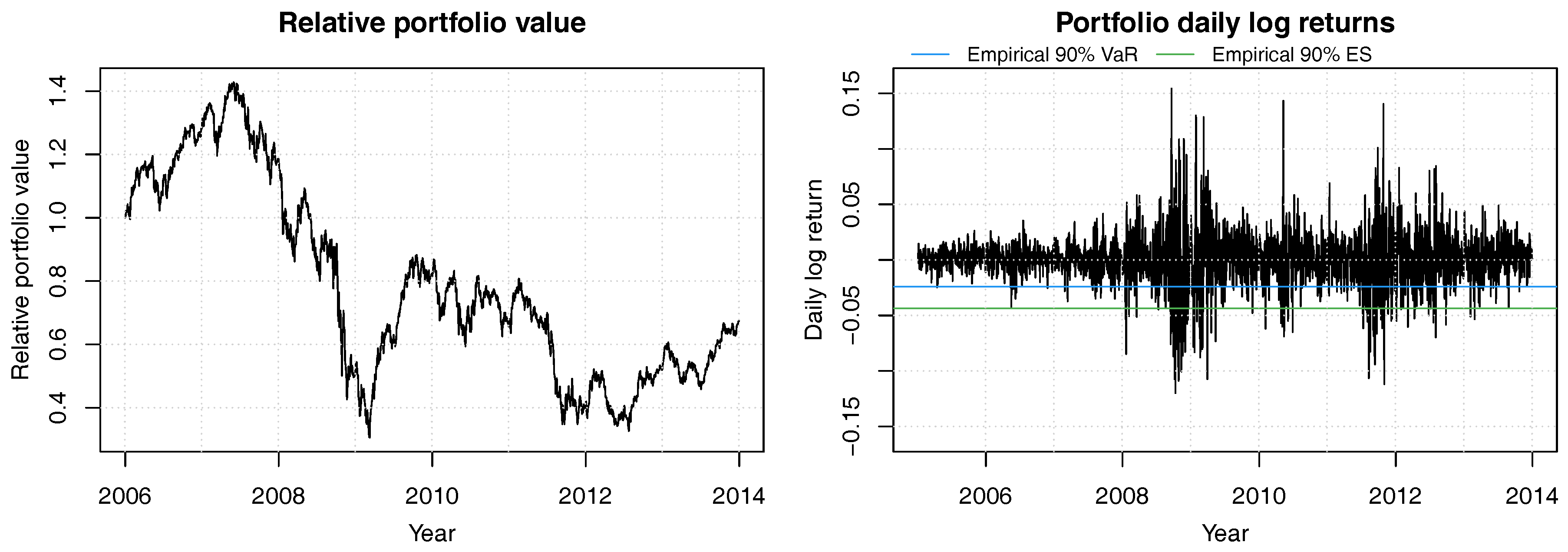
We use a constant mix strategy with equal weights in all stocks and daily re-balancing; this is without loss of generality. Figure 5 shows the portfolio value process of this portfolio. After an initial gain of more than 40%, the portfolio value plunged to less 50% of the initial value, and never fully recovered to pre-crisis highs; it should be noted that the dismal performance of this portfolio is the result of investing in financials exclusively, and not the result of an overly poor portfolio weights strategy.

Value at Risk Forecasts

Figure 6 shows the dynamic VaR forecasts provided by our Gaussian latent factor copula (in conjunction with marginal time series DLMs); our VaR forecasts are the 10% quantiles of each day’s 1,000 simulated portfolio returns. This figure shows that our dynamic combined multivariate time series model adapts quickly to changing market volatilities and eliminates the clustered occurrence of VaR violations found in an empirical constant volatility model (see right sub-figure of Figure 5). The realized frequency of VaR violations at the predicted levels was closest to the theoretical value of 10% for forecasts from the Bayesian Gumbel latent factor copula (10.17%), followed by the frequentist Gumbel latent factor copula (10.60%), and the regular vine copula (9.64%); furthermore, the Bayesian version of the latent factor copula always out-performed the frequentist version with the same choice of linking copula (Table 8).
In further analyses, we utilized the conditional coverage test suggested by (Christoffersen 2011, Chapter 13) to evaluate the performance of our models’ VaR forecasts. This test jointly analyzes the rate of VaR violations as well as whether they occur independently. Specifically, the null hypothesis of this test is that the hit sequence of ( 1 α % ) VaR violations is a first-order Markov chain, where violations happen with probability α and are independent of the current state of the chain. Again, the Bayesian latent factor copula with Gumbel linking copulas fares best, showing the highest p-value of 0.44 (Table 8). Most noteworthy is that all frequentist latent factor copula models can be rejected at the 10% level, while all Bayesian latent factor copulas and the Bayesian regular vine copula pass.
Although regulators often require higher confidence levels such as 99%, 99.5% or even 99.9%, producing robust estimates at these levels is not statistically feasible unless unrealistically big training data is available (see, e.g., McNeil et al. 2005, Example 7.15). In our study, no reliable results could be obtained about such extreme quantiles.

Expected Shortfall Forecasts

The empirical 90% ES of our equal weights portfolio from 2006 through 2014 was 4.58%, and the forecasts range between 4.00% and 4.13% for Bayesian latent factor copulas, 3.88% and 3.08% for frequentist latent factor copulas, and 4.07% for the regular vine copula (Table 8).
There are no universally accepted backtests for ES, as academic and regulatory discussions are ongoing (Embrechts et al. 2014). Part of the problem is that ES is not elicitable, which means that there is no obvious way to compare different ES forecasts. In this paper, we compare ES forecasts with the observed ES at the 90% level instead: using this decision criterion, our Bayesian latent factor model with survival Gumbel linking copulas yields performed best. Again, all frequentist latent factor copulas are out-performed by their Bayesian peers (Table 8).

6. Summary Comments

Latent factor copulas offer a simple and elegant way to parsimoniously model multivariate dependence and achieve scalability to high dimensions. Allowing for different choices of linking copulas, they provide sufficient flexibility to be used in a wide range of multivariate applications.
Our proposed Bayesian inference strategy utilizes adaptive rejection Metropolis sampling within Gibbs sampling for posterior simulation (Section 3). A main benefit to the end-user is that no tuning of MCMC proposals is required, given that ARMS is an adaptive method. At the same time, our analyses showed that adaptive rejection Metropolis sampling within Gibbs sampling (“ARMGS” in earlier sections) is a potent strategy that out-performed regular Metropolis-Hastings samplers with ease (see Section 4).
Our case study on forecasting the portfolio Value at Risk (VaR) and Expected Shortfall (ES) demonstrated that Bayesian latent factor copulas generated substantially improved risk forecasts than frequentist ones, and also out-performed the benchmark regular vine copula in terms of forecast accuracy (Section 5). We expect that these findings will impact industry best practices as well as regulatory requirements to potentially increase resilience of world financial markets.
Methods for model selection of linking copulas as well as time-varying extensions of the latent factor copula model are the subject of ongoing research. For example, we could potentially expect that the dependence parameters of the linking copulas change over time. Furthermore, Bayesian extensions allowing for several latent factors and/or structured factor copulas as proposed in Krupskii and Joe (2015) are future research directions.

Acknowledgments

The third author is supported by the German Research Foundation (DFG grant CZ 86/4-1). The authors are grateful to the Academic Editor and two anonymous referees for their detailed comments on the original version of the paper. Their suggestions were most relevant in revision and in defining the final version.

Author Contributions

All authors contributed equally.

Conflicts of Interest

The authors declare no conflict of interest.

Appendix A. MCMC Sampling Methods

Appendix A.1. Details on MCMC Sampling Schemes

Mode and Curvature Matching (MCM)

This strategy uses B e t a ( α t , β t ) -distributed ( α t , β t > 0 ) proposal distributions for each latent factor v t ( 0 , 1 ) , and a truncated normal distribution N [ a , b ] ( μ j , σ j 2 ) for the Fisher z parameters z j of each linking copula.
The mode and curvature of the B e t a ( α t , β t ) distribution with density f ( v t ; α t , β t ) are
mode v t ( α t , β t ) = α t 1 α t + β t 2 for α t , β t > 1 ; and curv v t ( v t , α t , β t ) : = 2 f ( v t ; α t , β t ) v t 2 = 1 B ( α t , β t ) v t α t 3 ( 1 v t ) β t 3 α t 2 + v t 2 ( α t + β t 3 ) ( α t + β t 2 ) 2 ( α t 1 ) v t ( α t + β t 3 ) 3 α t + 2 .
The mode and curvature of the truncated normal N [ a , b ] ( μ j , σ j 2 ) proposals for z j are
mode z j ( μ j ) = μ j for a μ j b ; and curv z j ( z j , μ j , σ j ) = e ( z j μ j ) 2 2 σ j 2 ( μ j 2 σ j 2 + z j 2 2 μ j z j ) 2 π σ j 5 Φ b z j σ j Φ a z j σ j for z j [ a , b ] .
Numerically unstable behavior of the copula density functions at perfect dependence requires truncation of the allowable parameter range of the linking copulas. We limit the range of allowable Kendall’s τ to [ 0 , 0.99 ] , which translates to allowable Fisher z parameters z j [ z ( 0 ) , z ( 0.99 ) ] = : [ a , b ] .
The proposal parameters α t , β t , μ j and σ j 2 are chosen such that the mode and curvature of the proposal distributions agree with the ones of the respective full conditional distributions. The calculations are performed using numerical methods.

Expectation and Variance Matching (EVM)

This strategy is basically the same as the previous one, but it matches the proposals’ and full conditionals’ expectation and variances instead of their modes and curvatures. In another deviation from the previous approach, we use G a m m a -distributed proposals for the Fisher z parameters here instead of truncated normal proposals used above.
The expectation and variance of the B e t a ( α t , β t ) proposals for the latent factor v t are
E v t ( α t , β t ) = α t α t + β t ; and V v t ( α t , β t ) = α t β t ( α t + β t ) 2 ( α t + β t + 1 ) .
Given expectation 0 < E v t < 1 and variance 0 < V v t < of the full conditional distribution of v t , this simple functional form enables analytic solution for the parameters α t and β t of the proposal distribution:
α t = E v t ( E v t 2 E v t + V v t ) V v t ; and β t = α t 1 E v t 1 .
For non-negative Fisher z parameters z j , j = 1 : d , of the linking copulas, we utilize G a m m a ( s j , r j ) -distributed proposals, s j , r j > 0 , with expectation and variance
E z j ( s j , r j ) = s j r j ; and V z j ( s j , r j ) = s j r j 2 .
Given expectation 0 < E z j < and variance 0 < V z j < of the full conditional distribution of z j , the proposal parameters s j and r j follow as
s j = E z j 2 V z j ; and r j = s j E z j .
Again, the expectation and variance of the full conditional distributions are evaluated using a numerical scheme.

Independence and Random Walk Samplers (IRW)

A numerically less complex alternative to the previous methods, this strategy employs an independence sampler for the latent factors v t , t = 1 : T , and a random walk sampler for the Fisher z parameters z j , j = 1 : d .
Proposals for each latent factor v t are drawn from a U n i f ( 0 , 1 ) distribution, and are independent of the current state of the sampling chain.
The proposal for the ( r + 1 ) -st iteration z j r + 1 of parameter z j is drawn from a truncated normal distribution N [ a , b ] ( μ j r + 1 , σ j 2 ) with random walk means μ j r + 1 = z j r . The proposal variances σ j 2 are chosen such that the acceptance rate is roughly 23 % , which is the optimal acceptance rate for multivariate normal random walk proposals (Roberts et al. 1997).

Adaptive Rejection Metropolis within Gibbs Sampling (ARMGS)

The last sampling method is adaptive rejection Metropolis sampling (ARMS) from the full conditionals of each variable v t , t = 1 : T , and z j , j = 1 : d ; this strategy is called adaptive rejection Metropolis sampling within Gibbs sampling (ARMGS; Gilks et al. (1995)). ARMS extends acceptance rejection sampling by a adaptive exponential envelope and a Metropolis-Hastings acceptance/rejection step. The acceptance/rejection step ensures proper sampling in case of a density that is not fully covered by the exponential envelope.
A major advantage of ARMS is that it adapts automatically to characteristics of the target distribution. For univariate log-concave target densities, ARMS creates an envelope for rejection sampling, while for other univariate target densities, ARMS uses acceptance/rejection sampling. In spite of being applicable to sample from general univariate target distributions, ARMS demonstrates good performance in many situations and is particularly appealing in the context of Gibbs sampling with complex full conditional distributions.
Block ARMS is a multivariate extension to ARMS. Instead of sampling each v t , t = 1 : T , and z j , j = 1 : d , individually, some or all of them can be sampled jointly from their multivariate block full conditional distribution. As this strategy did not perform well in our initial analyses (Schamberger 2015, Chapter 8), we will not discuss it here.

Appendix A.2. Strategy to Find Starting Values for MCMC

All methods discussed above require starting values for all parameters v and z . Good starting values can improve convergence speed of these MCMC methods and can also be used as an initial values for maximum likelihood estimation.
We propose a two-step heuristic that first chooses starting values for the Fisher z parameters z of the linking copulas, and then chooses starting values for the latent factor v .

Starting Values for z:

In order to estimate z , one series j { 1 , , d } is chosen as a proxy for latent factor v . We do this by selecting the 1-truncated c-vine copula that maximizes the sum of absolute Kendall’s τ ’s of all linking copulas and choosing the root node variable j * of this c-vine as the proxy for v . The starting values of the Fisher z parameters z j * = ( z j ) j { 1 : d } \ { j * } are set to the Fisher z parameter of the pair copula linking the corresponding series u : , j , j { 1 : d } \ { j * } , with the root node variable u : , j * . For the Fisher z parameter z j * of the linking copula that connects the root node variable u : , j * to the latent factor v , we use the highest absolute value of Fisher z parameters appearing in the c-vine as the starting value.

Starting Values for v:

Given starting values for the Fisher z parameters z , we set the latent factors v = ( v 1 , , v T ) to the modes of their full conditional densities.

Formal Procedure:

We generate starting values for posterior sampling of z and v , given T observations of d-dimensional data u = ( u t , : ) t = 1 : T with uniform marginals as follows.
  • Calculate the empirical d × d Kendall’s τ matrix T = ( τ i j ) i = 1 : d , j = 1 : d , where τ i j denotes the empirical Kendall’s τ between series u : , i and u : , j .
  • Find the column j * of T that maximizes the sum of absolute Kendall’s τ ’s,
    j * = arg max j = 1 : d i = 1 : d | τ i j |
  • Set the starting values z 0 = ( z 1 0 , , z d 0 ) for the Fisher z parameters z of the linking copulas to
    z i 0 = z τ i j * for i { 1 : d } \ { j * } z j * 0 = z max i = { 1 : d } \ { j * } τ i j *
  • Set the starting values v 0 = ( v t 0 ) t = 1 : T of the latent factor v to
    v t 0 = arg max v ( 0 , 1 ) p ( v | u t , z 0 ) ,
    where p is the full conditional density of v t given by (12).

Appendix B. Detailed Simulation Results

Table A1. Mean absolute deviation (MAD), mean squared errors (MSE), effective sample size (ESS) per minute, and coverage of 90% and 95% credible intervals for Kendall’s τ posterior sample. Results are averages over 100 independent replications of the analysis.
Low τ High τ Mixed τ
ARMGSMCMEVMIRWMLEARMGSMCMEVMIRWMLEARMGSMCMEVMIRWMLE
τ 1 MAD0.08290.07620.08980.08290.06560.03590.03520.03590.03570.02600.04310.04270.04320.04310.0321
MSE0.02030.01040.02690.02030.00990.00200.00200.00200.00200.00110.00290.00280.00290.00290.0016
ESS/min9.50.50.313.7n/a37.22.52.135.5n/a46.83.11.660.2n/a
90% C.I.0.920.650.930.92n/a0.890.880.890.88n/a0.970.960.970.97n/a
95% C.I.0.970.760.960.95n/a0.940.940.940.94n/a0.980.980.970.98n/a
τ 2 MAD0.09360.08320.08310.09160.06520.03340.03380.03350.03360.02590.04870.04860.04830.04920.0388
MSE0.02460.01160.01560.02290.00760.00170.00180.00170.00180.00100.00370.00370.00360.00380.0022
ESS/min7.90.60.211.6n/a33.22.21.831.5n/a37.62.91.846.7n/a
90% C.I.0.910.580.920.89n/a0.830.810.840.81n/a0.850.850.870.82n/a
95% C.I.0.960.670.960.93n/a0.920.880.920.92n/a0.920.910.920.92n/a
τ 3 MAD0.10700.09130.11440.09300.08110.02760.02790.02760.02770.01980.04060.03990.04070.04060.0290
MSE0.02980.01310.03540.01630.01370.00120.00120.00120.00120.00060.00260.00250.00260.00260.0013
ESS/min5.10.50.28.1n/a25.91.81.523.9n/a19.12.21.531.1n/a
90% C.I.0.910.500.860.88n/a0.900.870.900.90n/a0.870.870.860.84n/a
95% C.I.0.960.610.950.93n/a0.950.930.960.95n/a0.930.930.930.92n/a
τ 4 MAD0.11420.09830.11440.12310.07870.02520.02390.02540.02530.01720.04040.04010.04070.04010.0288
MSE0.03020.01450.03010.03690.01200.00100.00090.00100.00100.00050.00260.00250.00260.00260.0013
ESS/min4.70.60.26.8n/a15.71.21.014.4n/a2.80.80.46.8n/a
90% C.I.0.880.420.890.83n/a0.860.860.860.87n/a0.840.740.860.82n/a
95% C.I.0.940.490.910.89n/a0.930.900.920.93n/a0.890.790.890.86n/a
τ 5 MAD0.14630.10080.15070.12510.07870.02410.02490.02440.02450.01700.08170.04590.08550.08010.0406
MSE0.05240.01500.05570.03460.00940.00090.00100.00100.00100.00040.00990.00340.01060.00940.0023
ESS/min3.30.50.15.6n/a6.70.40.45.8n/a0.80.40.11.0n/a
90% C.I.0.940.490.910.92n/a0.970.800.980.97n/a0.810.480.820.71n/a
95% C.I.0.980.510.930.94n/a1.000.921.001.00n/a0.930.570.920.81n/a

Appendix C. Sequential Learning of DLMs


Priors at time t:

The prior for the states ( θ j t , λ j t ) given time t 1 information set D t 1 is normal-gamma
( θ j t , λ j t ) | D t 1 N G ( a j t , R j t , r j t , c j t )
with parameters a j t R 3 , R j t R 3 × 3 , r j t , c j t > 0 . The normal-gamma distribution is
θ j t | λ j t , D t 1 N ( a j t , R j t / ( c j t λ j t ) )
λ j t | D t 1 G ( r j t / 2 , r j t c j t / 2 ) .

Forecasts at time t:

The unconditional forecast distribution of y j t given time t 1 information set D t 1 is obtained by integrating observation Equation (14) over the prior distribution of θ j t and λ j t :
y j t | D t 1 T r j t ( f j t , q j t ) ,
with degrees of freedom r j t , mean f j t = F j t a jt and variance factor q j t = F j t R j t F j t + c j t . Here T r j t ( f j t , q j t ) denotes a non-standard t distribution, which is a location-scale transformation of a t distribution with r j t degrees of freedom, T r j t :
T r j t ( f j t , q j t ) = f j t + q j t T r j t .

Posteriors at time t:

Upon observation of y j t , the posterior distribution of ( θ j t , λ j t ) given information set D t : = { D t 1 , y j t } is normal-gamma
( θ j t , λ j t ) | D t N G ( m j t , C j t , n j t , s j t )
with parameters m j t = a j t + A j t e j t , C j t = ( R j t A j t A j t q j t ) z j t , n j t = r j t + 1 , s j t = z j t c j t ; these can be calculated using the adaptive coefficient vector A j t = R j t F j t / q j t , forecast error e j t = y j t f j t , and volatility update factor z j t = ( r j t + e j t 2 / q j t ) / n j t .

Evolution to time t + 1:

The step-ahead prior for ( θ j , t + 1 , λ j , t + 1 ) given time t information set D t is normal-gamma
( θ j , t + 1 , λ j , t + 1 ) | D t N G ( a j , t + 1 , R j , t + 1 , r j , t + 1 , c j , t + 1 ) ,
where a j , t + 1 = m j t , R j , t + 1 = C j t / δ , r j , t + 1 = β n j t , c j , t + 1 = s j t , and β , δ ( 0,1 ) are discount factors. This normal-gamma distribution is obtained via normal evolution of θ j t in system Equation (A8) and beta discount evolution of λ j t in system Equation (A10).
The system equation for state vector θ j t is
θ j , t + 1 = θ j t + ω j , t + 1 , ω j , t + 1 N ( 0 , W j , t + 1 ) ,
where the innovation variances W j , t + 1 = ( 1 δ ) / δ C j t are set to inflate the posterior variance C j t by the reciprocal of discount factor δ :
R j , t + 1 = C j t + W j , t + 1 = C j t + 1 δ δ C j t = 1 δ C j t .
The precisions λ j t evolve through the application of Beta-shocks with discount factor β ,
λ j , t + 1 = γ j , t + 1 β λ j t , γ j , t + 1 B e t a β n j t 2 , ( 1 β ) n j t 2 .

References

  1. Basel Committee on Banking Supervision. 2006. International Convergence of Capital Measurement and Capital Standards: A Revised Framework Comprehensive Version. Basel: Bank for International Settlements. [Google Scholar]
  2. Basel Committee on Banking Supervision. 2011. Basel III: A global regulatory framework for more resilient banks and banking systems. Basel: Bank for International Settlements. [Google Scholar]
  3. Basel Committee on Banking Supervision. 2013. Fundamental Review of the Trading Book: A Revised Market Risk Framework. Basel: Bank for International Settlements. [Google Scholar]
  4. Burns, Arthur F., and Wesley C. Mitchell. 1946. Measuring Business Cycles. Cambridge: The National Bureau of Economic Research. [Google Scholar]
  5. Christoffersen, Peter F. 2011. Elements of Financial Risk Management. New York: Academic Press. [Google Scholar]
  6. Crouhy, Michel, Dan Galai, and Robert Mark. 2000. A comparative analysis of current credit risk models. Journal of Banking & Finance 24: 59–117. [Google Scholar]
  7. Czado, Claudia, Florian Gärtner, and Aleksey Min. 2011. Analysis of Australian electricity loads using joint Bayesian inference of D-Vines with autoregressive margins. In Dependence Modeling: Vine Copula Handbook. Singapore: World Scientific Publishing, pp. 265–80. [Google Scholar]
  8. Dißmann, Jeffrey, Eike Christian Brechmann, Claudia Czado, and Dorota Kurowicka. 2013. Selecting and estimating regular vine copulae and application to financial returns. Computational Statistics & Data Analysis 59: 52–69. [Google Scholar]
  9. Embrechts, Paul, Er Mcneil, and Daniel Straumann. 1999. Correlation: Pitfalls and Alternatives. Available online: http://citeseerx.ist.psu.edu/viewdoc/summary?doi=10.1.1.638.3329 (accessed on 24 June 2014).
  10. Embrechts, Paul, Giovanni Puccetti, Ludger Rüschendorf, Ruodu Wang, and Antonela Beleraj. 2014. An academic response to Basel 3.5. Risks 2: 25–48. [Google Scholar] [CrossRef]
  11. European Parliament and Council. 2009. On the Taking-Up and Pursuit of the Business of Insurance and Reinsurance (Solvency II). Official Journal of the European Union 58: 10. [Google Scholar]
  12. Forni, Mario, Marc Hallin, Marco Lippi, and Lucrezia Reichlin. 2000. The generalized dynamic-factor model: Identification and estimation. Review of Economics and Statistics 82: 540–54. [Google Scholar] [CrossRef]
  13. Forni, Mario, Marc Hallin, Marco Lippi, and Lucrezia Reichlin. 2012. The generalized dynamic factor model. Journal of the American Statistical Association 100: 830–40. [Google Scholar] [CrossRef]
  14. Frey, Rüdiger, and Alexander J. McNeil. 2003. Dependent defaults in models of portfolio credit risk. Journal of Risk 6: 59–92. [Google Scholar] [CrossRef]
  15. Geweke, John. 1978. The Dynamic Factor Analysis of Economic Time Series Models. Madison: University of Wisconsin. [Google Scholar]
  16. Gelfand, Alan E., and Adrian F. M. Smith. 1990. Sampling-Based Approaches to Calculating Marginal Densities. Journal of the American Statistical Association 85: 398–409. [Google Scholar] [CrossRef]
  17. Gilks, Wally R., Nicola G. Best, and Keith K.C. Tan. 1995. Adaptive rejection Metropolis sampling within Gibbs sampling. Applied Statistics 44: 455–73. [Google Scholar] [CrossRef]
  18. Gordy, Michael B. 2000. A comparative anatomy of credit risk models. Journal of Banking & Finance 24: 119–49. [Google Scholar]
  19. Gruber, Lutz, and Claudia Czado. 2015. Sequential Bayesian Model Selection of Regular Vine Copulas. Bayesian Analysis 10: 937–63. [Google Scholar] [CrossRef]
  20. Gruber, Lutz, and Mike West. 2016. GPU-Accelerated Bayesian Learning and Forecasting in Simultaneous Graphical Dynamic Linear Models. Bayesian Analysis 11: 125–49. [Google Scholar] [CrossRef]
  21. Hastings, W. Keith. 1970. Monte Carlo sampling methods using Markov chains and their applications. Biometrika 57: 97–109. [Google Scholar] [CrossRef]
  22. Joe, Harry. 1997. Multivariate Models and Multivariate Dependence Concepts. New York: CRC Press. [Google Scholar]
  23. Joe, Harry, and James Jianmeng Xu. 1996. The Estimation Method of Inference Functions for Margins for Multivariate Models. Technical Report No. 166. Vancouver: Department of Statistics, University of British Columbia. [Google Scholar]
  24. Joe, Harry. 2005. Asymptotic efficiency of the two-stage estimation method for copula-based models. Journal of Multivariate Analysis 94: 401–19. [Google Scholar] [CrossRef]
  25. Krupskii, Pavel, and Harry Joe. 2013. Factor copula models for multivariate data. Journal of Multivariate Analysis 120: 85–101. [Google Scholar] [CrossRef]
  26. Krupskii, Pavel, and Harry Joe. 2015. Structured factor copula models: Theory, inference and computation. Journal of Multivariate Analysis 138: 53–73. [Google Scholar] [CrossRef]
  27. McNeil, Alexander J., Rüdiger Frey, and Paul Embrechts. 2005. Quantitative Risk Management: Concepts, Techniques, and Tools. Princeton: Princeton University Press. [Google Scholar]
  28. Metropolis, Nicholas, Arianna W. Rosenbluth, Marshall N. Rosenbluth, Augusta H. Teller, and Edward Teller. 1953. Equation of State Calculations by Fast Computing Machines. Journal of Chemical Physics 21: 1087–92. [Google Scholar] [CrossRef]
  29. Murray, Jared S., David B. Dunson, Lawrence Carin, and Joseph E. Lucas. 2013. Bayesian Gaussian Copula Factor Models for Mixed Data. Journal of the American Statistical Association 108: 656–65. [Google Scholar] [CrossRef] [PubMed]
  30. Oh, Dong Hwan, and Andrew J. Patton. 2017. Modelling dependence in high dimensions with factor copulas. Journal of Business & Economic Statistics 35: 139–54. [Google Scholar]
  31. Roberts, Gareth O., Andrew Gelman, and Walter R. Gilks. 1997. Weak convergence and optimal scaling of random walk Metropolis algorithms. The Annals of Applied Probability 7: 110–20. [Google Scholar] [CrossRef]
  32. Sargent, Thomas J., and Christopher A. Sims. 1977. Business cycle modeling without pretending to have too much a priori economic theory. New Methods in Business Cycle Research 1: 145–68. [Google Scholar]
  33. Schepsmeier, Ulf, Jakob Stoeber, Eike Christian Brechmann, and Benedikt Graeler. 2014. VineCopula: Statistical Inference of Vine Copulas, R Package Version 1.3.
  34. Schamberger, Benedikt. 2015. Bayesian Analysis of the One-Factor Copula Model with Applications to Finance. Master’s dissertation, Technische Universität München, München, Germany. Available online: http://mediatum.ub.tum.de/doc/1253486/1253486.pdf (accessed on 4 January 2016).
  35. Sklar, Abe. 1959. Fonctions de Répartition À N Dimensions et Leurs Marges. Paris: Publications de L’Institut de Statistique de l’Université de Paris, vol. 8, pp. 229–31. [Google Scholar]
  36. Thiébaux, H. Jean, and Francis W. Zwiers. 1984. The interpretation and estimation of effective sample size. Journal of Climate and Applied Meteorology 23: 800–11. [Google Scholar] [CrossRef]
  37. West, Mike, and Jeff Harrison. 1997. Bayesian Forecasting & Dynamic Models, 2nd ed. New York: Springer Verlag. [Google Scholar]
Figure 1. Trace plots and density plots of a single run from each of our four sampling methods on Kendall’s τ scale. The output is based on 10,000 posterior samples of z 1 in the mixed τ scenario.
Econometrics 05 00021 g001
Figure 2. Daily log-returns (grey) of ACA from 2004 through 2013 with DLM one-day ahead 90% confidence bands (blue) and forecast value (dark blue).
Econometrics 05 00021 g002
Figure 3. Kendall’s τ posterior modes with corresponding 90% credible intervals of copula parameters of the latent factor copula model with Gumbel (red), Gaussian (blue) and survival Gumbel (green) linking copulas.
Econometrics 05 00021 g003aEconometrics 05 00021 g003b
Figure 4. Contour plots with standard normal margins for ACA and latent factor pairs ( u ACA , t , v ^ t ) for 2005 (Top) and 1 July 2008 to 30 June 2009 (Bottom). Empirical densities are indicated by solid black lines, while dotted blue lines show the theoretical densities.
Econometrics 05 00021 g004
Figure 5. Historical relative portfolio value of a constant mix strategy with equal weights in the 8 bank stocks ACA, BBVA, BNP, CBK, DBK, GLE, ISP and SAN for years 2006 to 2013. Portfolio weights are readjusted daily. The 90% empirical VaR is shown in blue and the 90% empirical ES is in green.
Econometrics 05 00021 g005
Figure 6. Daily log-returns of the equally weighted constant mix portfolio with (negative) 90% VaR (blue line) and ES (green line) forecasts.
Econometrics 05 00021 g006
Table 1. Density functions and Kendall’s τ as a function of the parameter of the Gaussian and Gumbel pair copulas.
CopulaDensity Function τ = h ( θ )
Gaussian c N ( u 1 , u 2 ; θ ) = 1 1 δ 2 2 π ϕ ( Φ 1 ( u 1 ) ) ϕ ( Φ 1 ( u 2 ) ) × exp Φ 1 ( u 1 ) + Φ 1 ( u 2 ) 2 δ Φ 1 ( u 1 ) Φ 1 ( u 2 ) 2 ( 1 δ 2 ) h N ( θ ) = 2 π arcsin ( θ )
Gumbel c G ( u 1 , u 2 ; θ ) = 1 u 1 u 2 x 1 x 2 θ 1 × exp x 1 θ x 2 θ θ × ( 1 θ ) x 1 θ x 2 θ 1 θ 2 + x 1 θ x 2 θ 2 θ 2 , where x 1 = ln u 1 and x 2 = ln u 2 h G ( θ ) = 1 1 θ
Survival Gumbel c SG ( u 1 , u 2 ; θ ) = c G ( 1 u 1 , 1 u 2 ; θ ) h SG ( θ ) = 1 1 θ
Table 2. Pairs plots for the Gaussian, Gumbel and survival Gumbel copulas for different parameter values. As the Gumbel and survival Gumbel copulas only exhibit positive dependence, the 90 and 270 rotations of the Gumbel copulas are shown for negative Fisher z parameters.
Fisher’s z z = 1.2 z = 0.5 z = 0.7 z = 1
Gaussian Econometrics 05 00021 i001 Econometrics 05 00021 i002 Econometrics 05 00021 i003 Econometrics 05 00021 i004
Gumbel Econometrics 05 00021 i005 Econometrics 05 00021 i006 Econometrics 05 00021 i007 Econometrics 05 00021 i008
Survival Gumbel Econometrics 05 00021 i009 Econometrics 05 00021 i010 Econometrics 05 00021 i011 Econometrics 05 00021 i012
Table 3. Copula parameters used in the simulation to model the dependence between each marginal series u : , j : = ( u 1 j , , u T j ) and the latent factor v .
c 1 c 2 c 3 c 4 c 5
Low τ
τ 0.100.120.150.180.20
θ 1.111.141.181.211.25
z0.100.130.150.180.20
High τ
τ 0.500.570.650.730.80
θ 2.002.352.863.645.00
z0.550.650.780.921.10
Mixed τ
τ 0.100.280.450.620.80
θ 1.111.381.822.675.00
z0.100.280.480.731.10
Table 4. Mean absolute deviation (MAD), mean squared error (MSE), effective sample size (ESS) per minute, and realized coverage of 95% credible intervals (C.I.) averaged across all variables τ 1 , , τ 5 and N = 100 replications. Runtime is for 10,000 MCMC iterations on a 16-core node.
ARMGSMCMEVMIRWMLE
Low τ
MAD0.10880.09000.11050.10320.0739
MSE0.03140.01290.03270.02620.0105
ESS/min6.10.50.29.2n/a
95% C.I.0.960.610.940.93n/a
High τ
MAD0.02920.02920.02930.02940.0212
MSE0.00140.00140.00140.00140.0007
ESS/min23.71.61.422.2n/a
95% C.I.0.950.910.950.95n/a
Mixed τ
MAD0.05090.04340.05170.05060.0339
MSE0.00430.00300.00450.00420.0017
ESS/min21.41.91.129.2n/a
95% C.I.0.930.840.930.90n/a
Average across All Scenarios
Runtime165s664s776s55s
Table 5. Mean absolute deviation (MAD), mean squared error (MSE), effective sample size (ESS) per minute, and realized coverage of 95% credible intervals (C.I.) averaged across all latent variables v 1 , , v T and N = 100 replications.
ARMGSMCMEVMIRW
Low τ
MAD0.28080.29750.28050.2811
MSE0.12480.13970.12480.1251
ESS/min25.70.51.163.5
95% C.I.0.910.710.890.88
High τ
MAD0.07090.06780.07100.0709
MSE0.00950.00870.00950.0095
ESS/min43.71.62.638.8
95% C.I.0.950.800.950.94
Mixed τ
MAD0.08280.08980.08240.0826
MSE0.01320.01540.01310.0131
ESS/min25.81.52.034.3
95% C.I.0.880.780.870.83
Table 6. Ticker symbol, company name and exchange of the selected bank stocks.
TickerCompany NameExchange
ACA.PACredit Agricole S.A.Euronext - Paris
BBVA.MCBanco Bilbao Vizcaya ArgentariaMadrid Stock Exchange
BNP.PABNP Paribas SAEuronext - Paris
CBK.DECommerzbank AGXETRA
DBK.DEDeutsche Bank AGXETRA
GLE.PASociete Generale GroupEuronext - Paris
ISP.MIIntesa Sanpaolo S.p.A.Borsa Italiana
SAN.MCBanco SantanderMadrid Stock Exchange
Table 7. Percentage of observed log-returns above and below sequentially out-of-sample 90% forecast interval.
ACABBVABNPCBKDBKGLEISPSAN
Above 95% bound4.90%4.90%4.43%4.86%4.22%4.73%4.73%4.61%
Below 5% bound4.35%5.07%4.65%4.43%5.29%4.78%5.33%5.16%
Table 8. Frequency of 90% VaR violations and 90% ES of an equals weights portfolio of all eight selected financial stocks, and p-values of conditional coverage test of VaR violations. R V R denotes the multivariate regular vine copula model; the other columns are for the dynamic factor copula model with the respective linking copula families. The best values are emphasized in bold.
GumbelGaussianSurvival Gumbel
RV R ARMGSMLEARMGSMLEARMGSMLE
90% VaR viol.9.64%10.17%10.60%9.59%9.36%9.35%9.17%
90% ES4.07%4.00%3.88%4.10%4.08%4.13%4.08%
p-value, cond. coverage test0.240.440.070.300.010.100.03