
Brain Tumor Segmentation from Optimal MRI Slices Using a Lightweight U-Net

 , , , , , , and
Abstract
1. Introduction
- 1.
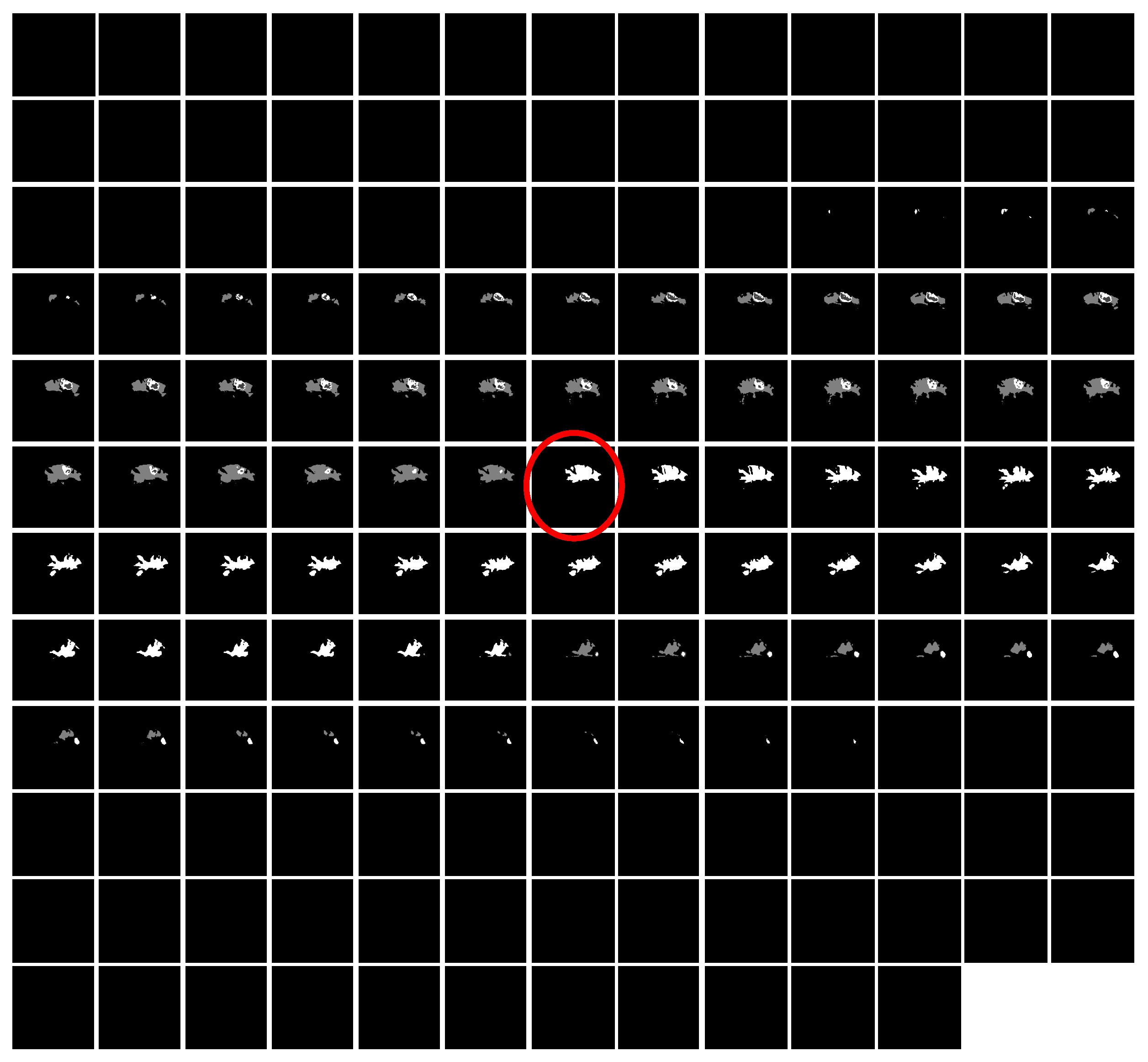
- An automatic preprocessing of 3D MRI images to extract the most significant cross-sectional T2 image modality.
- 2.
- A lightweight UNET for brain tumor segmentation.
- 3.
- Restructuring a modified and lightweight UNET network for biomedical image segmentation and tumor detection, particularly MRIs.
- 4.
- Optimizing UNET by reducing convolutional filters for a lighter and portable architecture.
- 5.
- Implementing an Adaptive Learning Rate strategy to minimize the cost function optimally.
2. Literature Review
3. Mathematical Background
3.1. Convolutional Layer
3.2. Pooling Layer
3.3. Dropout Layer
3.4. Batch Normalization
3.5. Activation Functions
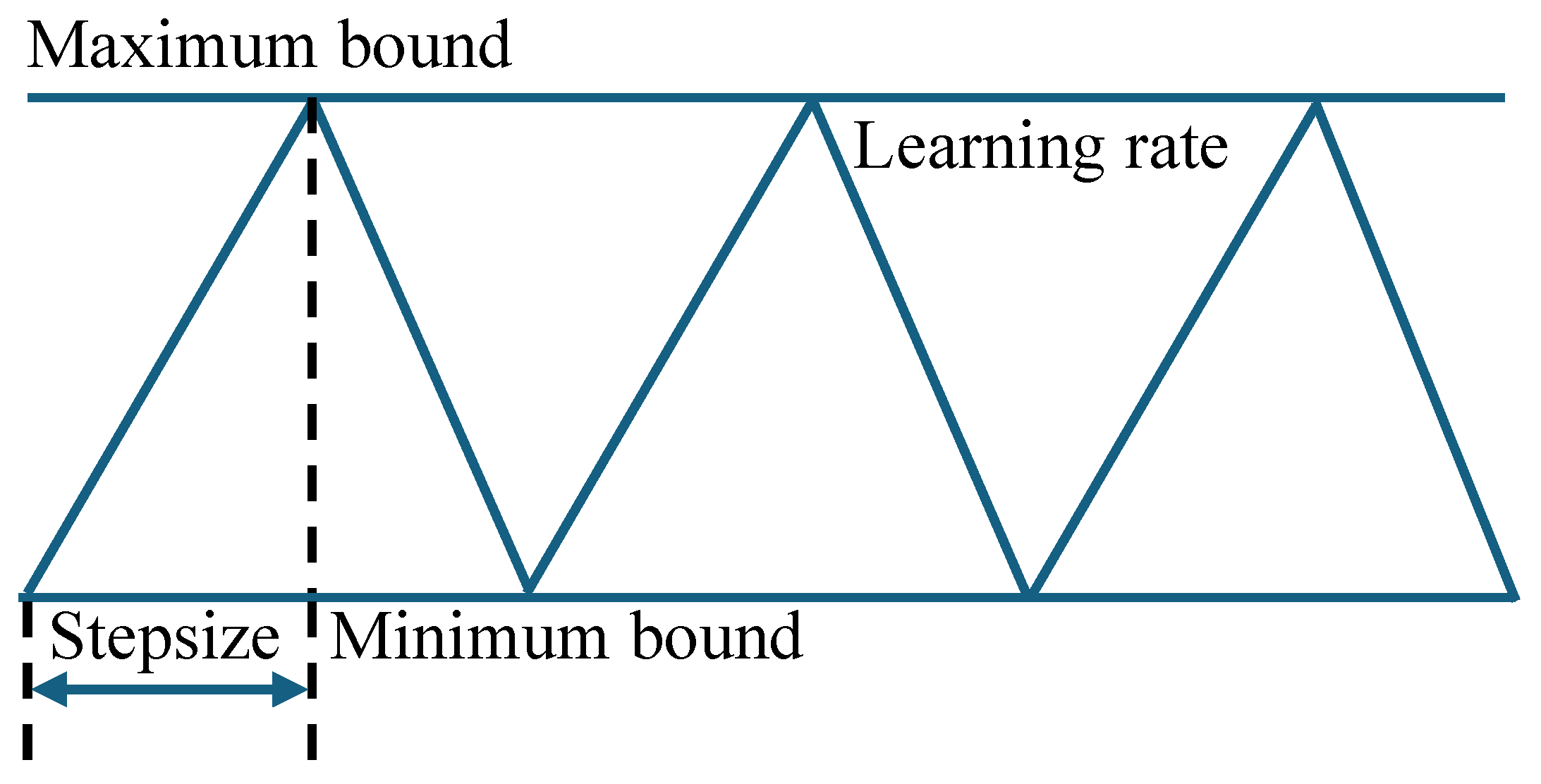
Cyclical Learning Rate
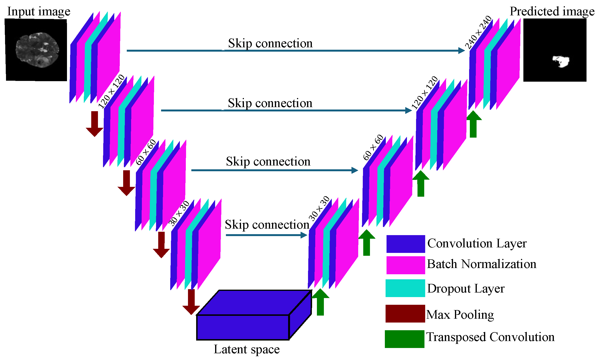
3.6. UNET Architecture
4. Materials and Method
4.1. BraTS Datasets
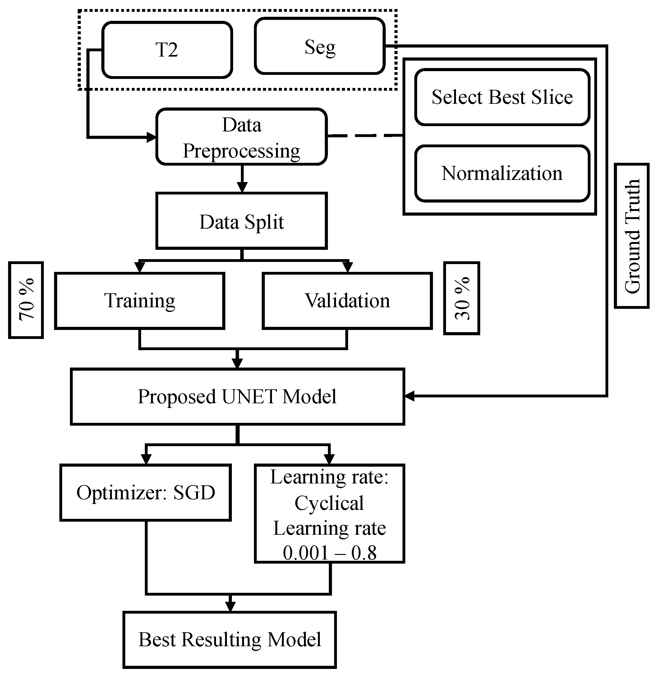
4.2. Overall Framework
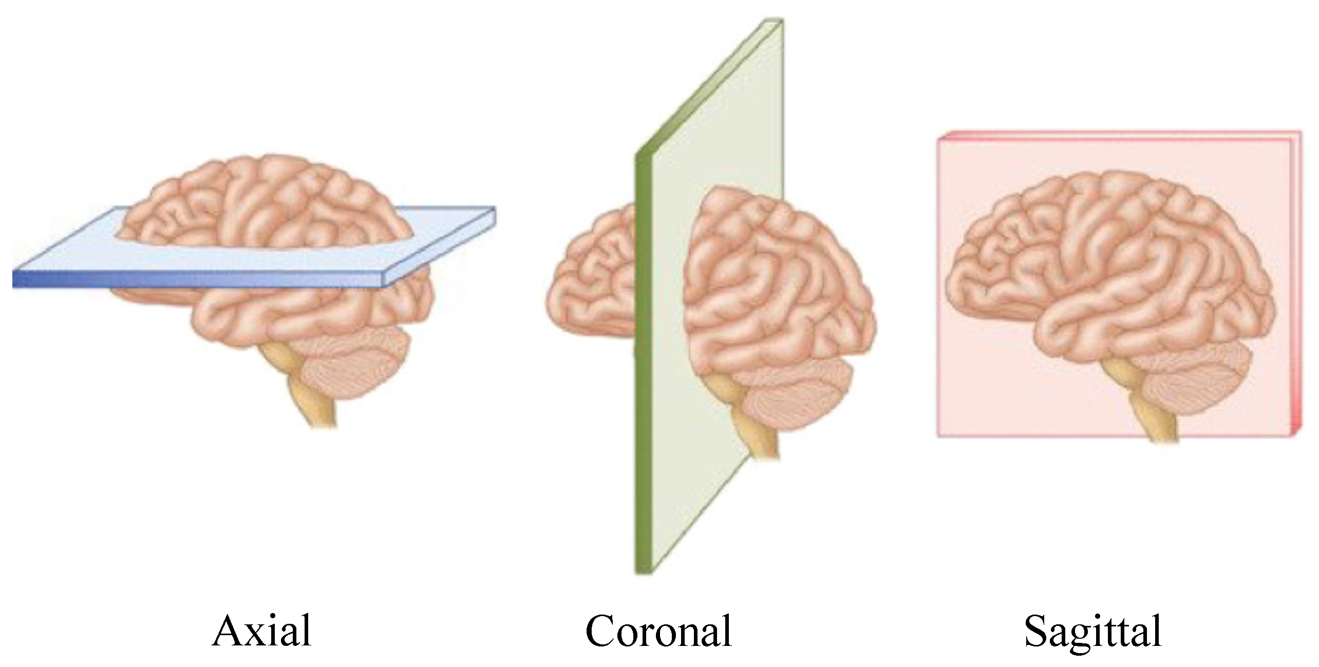
4.3. Data Prepossessing
4.4. Proposed Model
4.5. Implementation Details
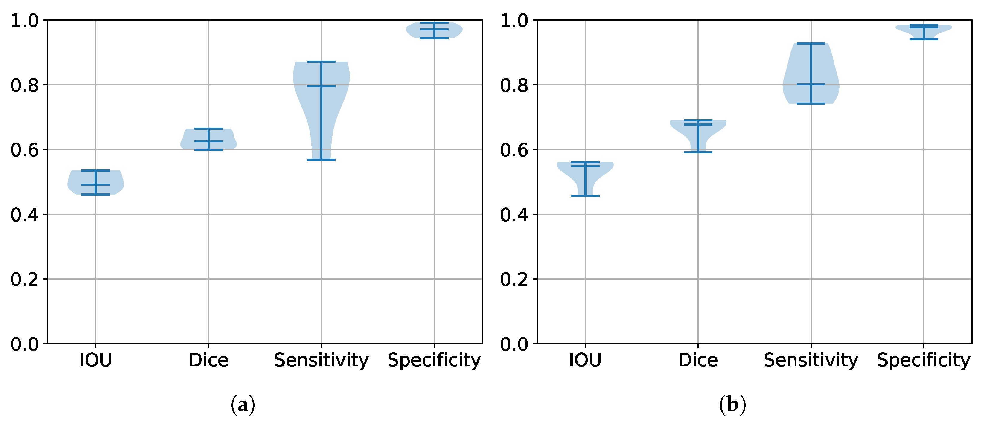
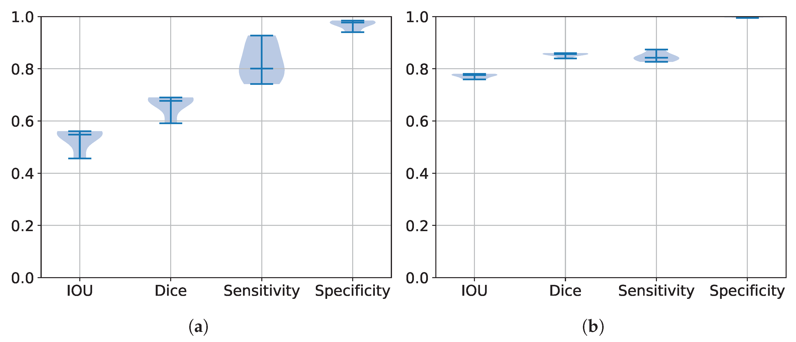
5. Numerical Results
5.1. Evaluations Metrics
5.1.1. Dice Similarity Coefficient
5.1.2. Intersection over Union
5.1.3. Sensitivity
5.1.4. Specificity
5.1.5. Hausdorff Distance
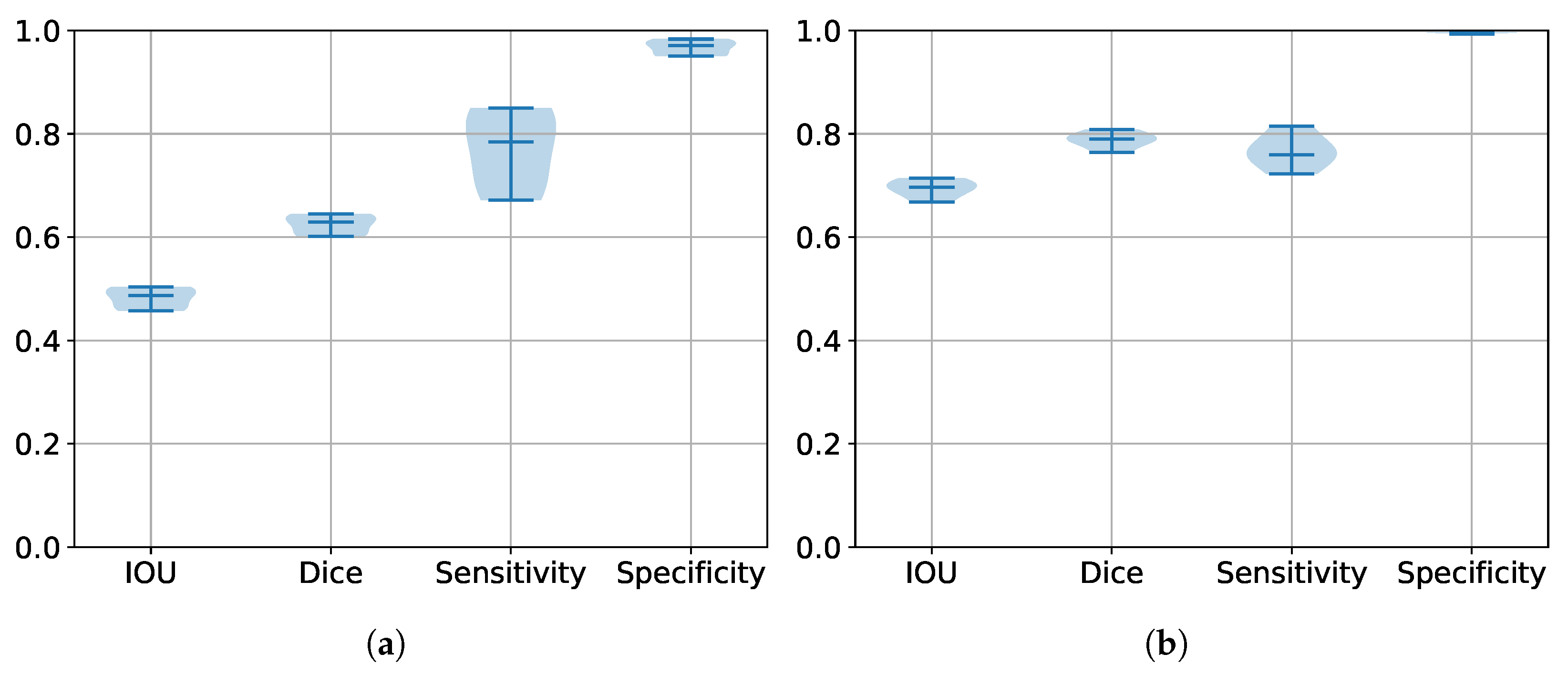
5.2. Performance Estimation of All Trained Models
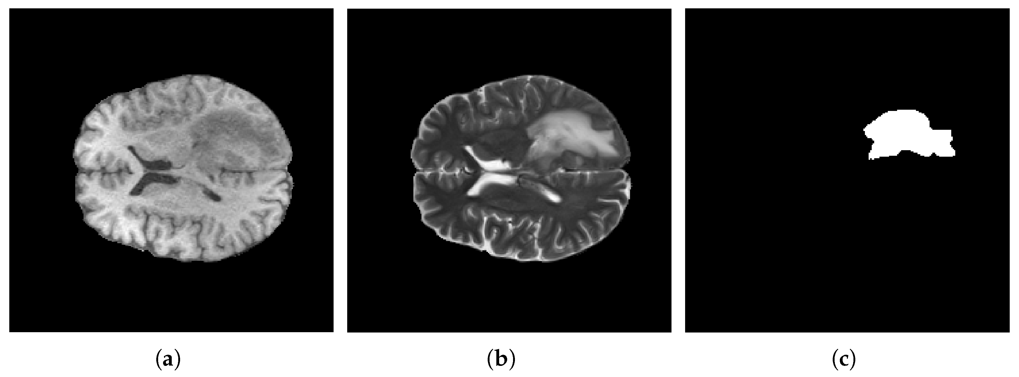
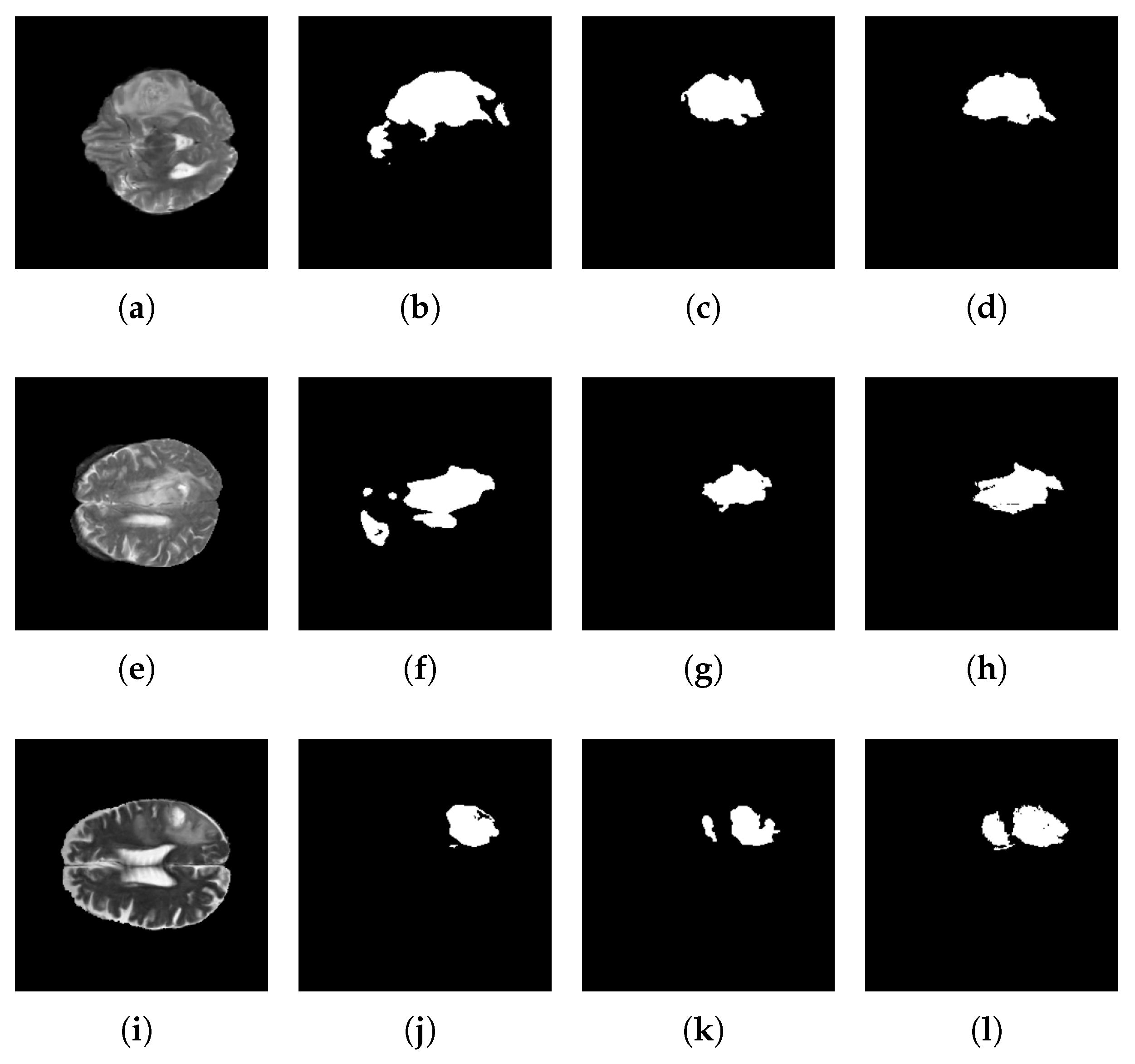
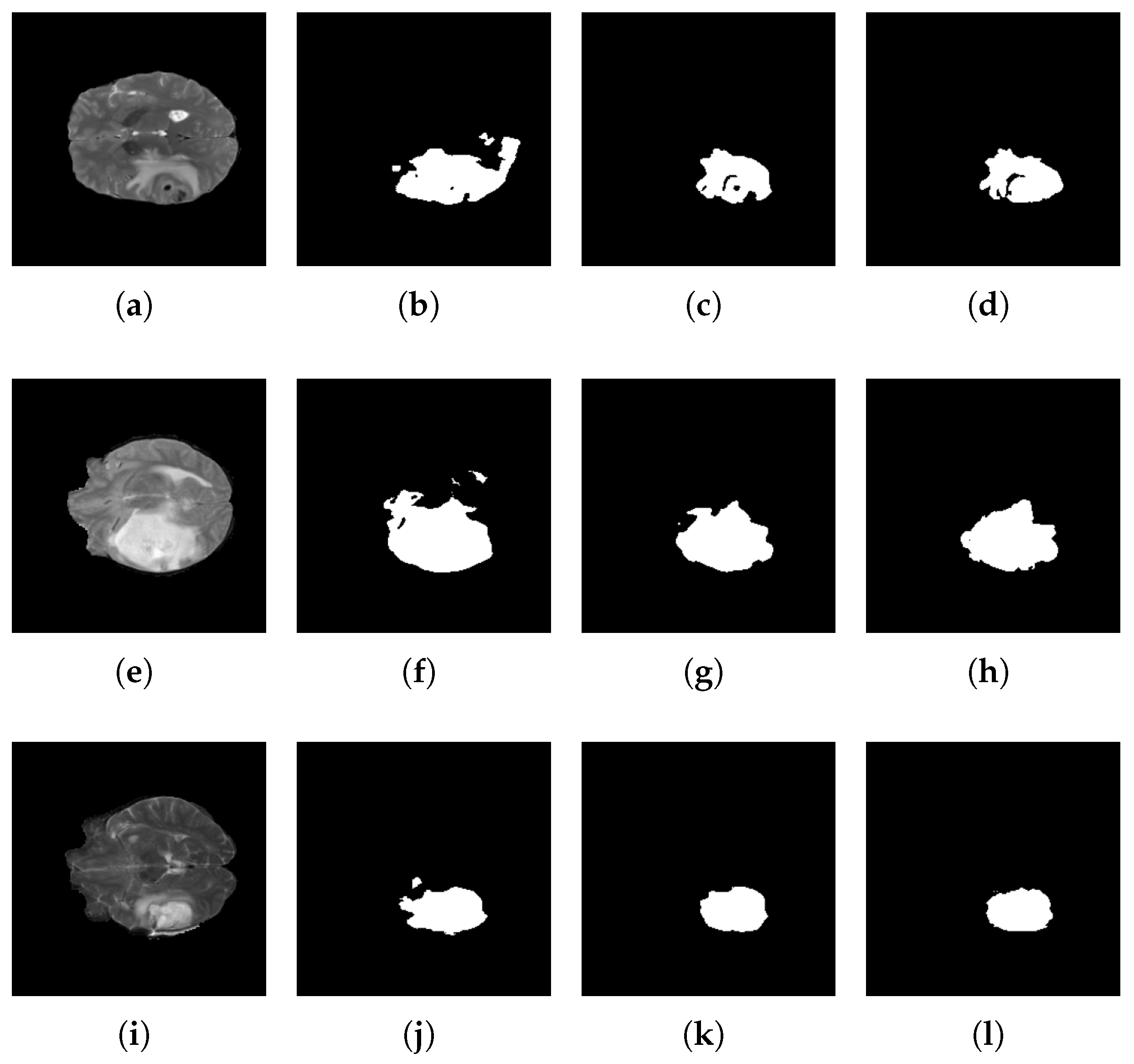
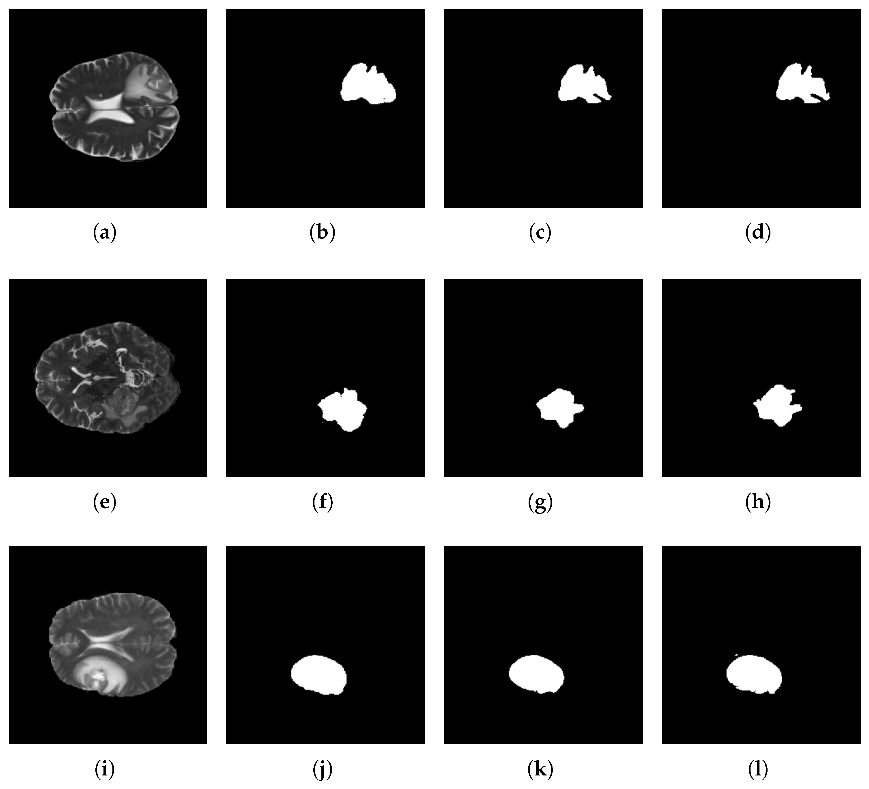
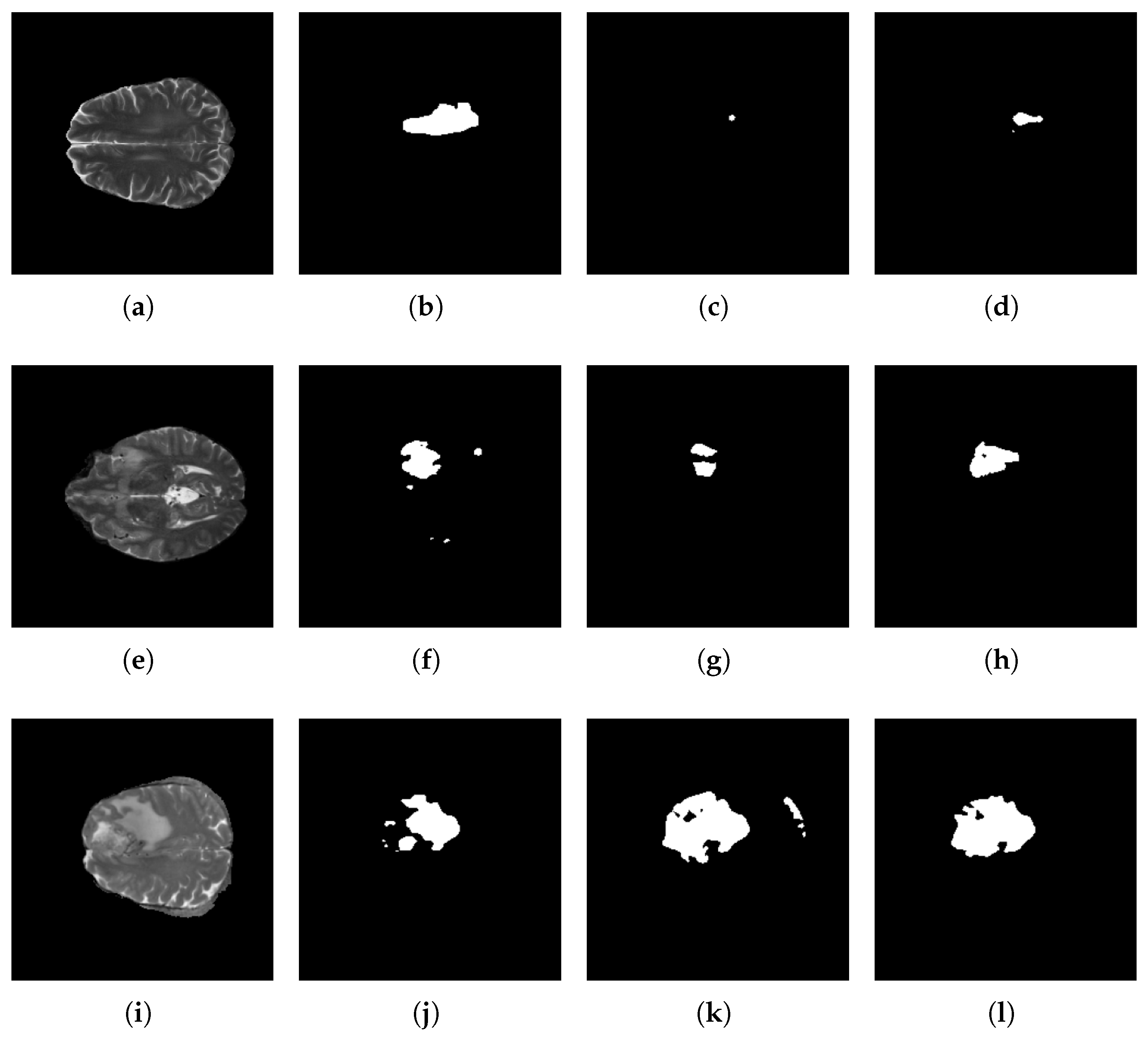
5.3. Segmentation Results

| Reference | IoU | DSC | HD | Sensitivity | Specificity | Params () | GFlops |
|---|---|---|---|---|---|---|---|
| Sun et al. [38] | - | 0.819 | 2.662 | 0.811 | - | 73.2 | |
| Xu et al. [39] | 0.703 | 0.788 | - | - | - | 6.08 | |
| Raza et al. [40] | - | 0.8601 | - | - | - | - | - |
| Akbar et al. [37] | - | 0.8933 | 15.83 | 0.9278 | - | - | - |
| Mokhtar et al. [36] | - | 0.903 | 9.9 | 0.96 | 0.99 | - | - |
| UNET++ | 0.78755 | 0.86705 | 18.2394 | 0.86363 | 0.99629 | 97.7 | |
| Base | 0.72527 | 0.80977 | 36.37064 | 0.77456 | 0.99738 | 84.5 | |
| Base (BN) | 0.70029 | 0.78856 | 13.5851 | 0.80518 | 0.98998 | 5.3 | |
| Base (BN & CLR) | 0.00691 | 0.01353 | 18.0803 | 0.14846 | 0.81738 | 5.3 | |
| Base (BN & CLR & SGD) | 0.57465 | 0.66023 | 12.2119 | 0.64639 | 0.99444 | 5.3 | |
| Base (BN & CLR & SGD & SeLU) | 0.78070 | 0.860 | 12.0603 | 0.856 | 0.9964 | 5.3 |
5.4. Discussion
6. Conclusions
Author Contributions
Funding
Institutional Review Board Statement
Informed Consent Statement
Data Availability Statement
Acknowledgments
Conflicts of Interest
References
- Hu, A.; Razmjooy, N. Brain tumor diagnosis based on metaheuristics and deep learning. Int. J. Imaging Syst. Technol. 2021, 31, 657–669. [Google Scholar] [CrossRef]
- Sharif, M.; Amin, J.; Raza, M.; Anjum, M.A.; Afzal, H.; Shad, S.A. Brain tumor detection based on extreme learning. Neural Comput. Appl. 2020, 32, 15975–15987. [Google Scholar] [CrossRef]
- International Agency for Research on Cancer. IARC Global Cancer Observatory. Available online: https://gco.iarc.who.int/today/en/dataviz/maps-heatmap?cancers=31&types=0&sexes=1&palette=Blues&mode=population (accessed on 29 April 2024).
- Badža, M.M.; Barjaktarović, M.Č. Classification of Brain Tumors from MRI Images Using a Convolutional Neural Network. Appl. Sci. 2020, 10, 1999. [Google Scholar] [CrossRef]
- Bhandari, A.; Koppen, J.; Agzarian, M. Convolutional neural networks for brain tumour segmentation. Insights Imaging 2020, 11, 77. [Google Scholar] [CrossRef] [PubMed]
- Walsh, J.; Othmani, A.; Jain, M.; Dev, S. Using U-Net network for efficient brain tumor segmentation in MRI images. Healthc. Anal. 2022, 2, 100098. [Google Scholar] [CrossRef]
- Shoaib, M.A.; Lai, K.W.; Chuah, J.H.; Hum, Y.C.; Ali, R.; Dhanalakshmi, S.; Wang, H.; Wu, X. Comparative studies of deep learning segmentation models for left ventricle segmentation. Front. Public Health 2022, 10, 981019. [Google Scholar] [CrossRef]
- Razzak, M.I.; Imran, M.; Xu, G. Efficient Brain Tumor Segmentation With Multiscale Two-Pathway-Group Conventional Neural Networks. IEEE J. Biomed. Health Inform. 2019, 23, 1911–1919. [Google Scholar] [CrossRef]
- Hao, K.; Lin, S.; Qiao, J.; Tu, Y. A Generalized Pooling for Brain Tumor Segmentation. IEEE Access 2021, 9, 159283–159290. [Google Scholar] [CrossRef]
- Aghalari, M.; Aghagolzadeh, A.; Ezoji, M. Brain tumor image segmentation via asymmetric/symmetric UNet based on two-pathway-residual blocks. Biomed. Signal Process. Control. 2021, 69, 102841. [Google Scholar] [CrossRef]
- Ottom, M.A.; Rahman, H.A.; Dinov, I.D. Znet: Deep Learning Approach for 2D MRI Brain Tumor Segmentation. IEEE J. Transl. Eng. Health Med. 2022, 10, 1800508. [Google Scholar] [CrossRef] [PubMed]
- Ahmad, P.; Jin, H.; Alroobaea, R.; Qamar, S.; Zheng, R.; Alnajjar, F.; Aboudi, F. MH UNet: A Multi-Scale Hierarchical Based Architecture for Medical Image Segmentation. IEEE Access 2021, 9, 148384–148408. [Google Scholar] [CrossRef]
- Latif, U.; Shahid, A.R.; Raza, B.; Ziauddin, S.; Khan, M.A. An end-to-end brain tumor segmentation system using multi-inception-UNET. Int. J. Imaging Syst. Technol. 2021, 31, 1803–1816. [Google Scholar] [CrossRef]
- Montaha, S.; Azam, S.; Rakibul Haque Rafid, A.K.M.; Hasan, M.Z.; Karim, A. Brain Tumor Segmentation from 3D MRI Scans Using U-Net. SN Comput. Sci. 2023, 4, 386. [Google Scholar] [CrossRef]
- Ranjbarzadeh, R.; Zarbakhsh, P.; Caputo, A.; Tirkolaee, E.B.; Bendechache, M. Brain tumor segmentation based on optimized convolutional neural network and improved chimp optimization algorithm. Comput. Biol. Med. 2024, 168, 107723. [Google Scholar] [CrossRef]
- Ghazouani, F.; Vera, P.; Ruan, S. Efficient brain tumor segmentation using Swin transformer and enhanced local self-attention. Int. J. Comput. Assist. Radiol. Surg. 2024, 19, 273–281. [Google Scholar] [CrossRef] [PubMed]
- Yue, G.; Zhuo, G.; Zhou, T.; Liu, W.; Wang, T.; Jiang, Q. Adaptive Cross-Feature Fusion Network with Inconsistency Guidance for Multi-Modal Brain Tumor Segmentation. IEEE J. Biomed. Health Inform. 2023, 1–11. [Google Scholar] [CrossRef]
- Baldi, P.; Sadowski, P. The dropout learning algorithm. Artif. Intell. 2014, 210, 78–122. [Google Scholar] [CrossRef] [PubMed]
- Santurkar, S.; Tsipras, D.; Ilyas, A.; Madry, A. How Does Batch Normalization Help Optimization? arXiv 2019, arXiv:1805.11604. [Google Scholar]
- Bjorck, J.; Gomes, C.P.; Selman, B. Understanding Batch Normalization. arXiv 2018, arXiv:1806.02375. [Google Scholar]
- Dubey, S.R.; Singh, S.K.; Chaudhuri, B.B. Activation functions in deep learning: A comprehensive survey and benchmark. Neurocomputing 2022, 503, 92–108. [Google Scholar] [CrossRef]
- Klambauer, G.; Unterthiner, T.; Mayr, A.; Hochreiter, S. Self-Normalizing Neural Networks. arXiv 2017, arXiv:1706.02515. [Google Scholar]
- Oymak, S. Provable Super-Convergence With a Large Cyclical Learning Rate. IEEE Signal Process. Lett. 2021, 28, 1645–1649. [Google Scholar] [CrossRef]
- Ronneberger, O.; Fischer, P.; Brox, T. U-Net: Convolutional Networks for Biomedical Image Segmentation. In Medical Image Computing and Computer-Assisted Intervention—MICCAI 2015; Navab, N., Hornegger, J., Wells, W.M., Frangi, A.F., Eds.; Springer: Cham, Switzerland, 2015; pp. 234–241. [Google Scholar] [CrossRef]
- Amin, J.; Sharif, M.; Raza, M.; Saba, T.; Anjum, M.A. Brain tumor detection using statistical and machine learning method. Comput. Methods Programs Biomed. 2019, 177, 69–79. [Google Scholar] [CrossRef] [PubMed]
- BraTS 2017: Multimodal Brain Tumor Segmentation Challenge. Available online: https://www.med.upenn.edu/sbia/brats2017/data.html (accessed on 2 January 2024).
- BraTS 2020: Multimodal Brain Tumor Segmentation Challenge. Available online: https://www.med.upenn.edu/cbica/brats2020/ (accessed on 2 January 2024).
- BraTS 2021: Multimodal Brain Tumor Segmentation Challenge. Available online: https://www.med.upenn.edu/cbica/brats2021/ (accessed on 2 January 2024).
- Smith, L.N. Cyclical learning rates for training neural networks. In Proceedings of the 2017 IEEE Winter Conference on Applications of Computer Vision, WACV 2017, Santa Rosa, CA, USA, 24–31 March 2017; pp. 464–472. [Google Scholar] [CrossRef]
- Zou, K.H.; Warfield, S.K.; Bharatha, A.; Tempany, C.M.; Kaus, M.R.; Haker, S.J.; Wells, W.M.; Jolesz, F.A.; Kikinis, R. Statistical validation of image segmentation quality based on a spatial overlap index1: Scientific reports. Acad. Radiol. 2004, 11, 178–189. [Google Scholar] [CrossRef] [PubMed]
- Zanddizari, H.; Nguyen, N.; Zeinali, B.; Chang, J.M. A new preprocessing approach to improve the performance of CNN-based skin lesion classification. Med. Biol. Eng. Comput. 2021, 59, 1123–1131. [Google Scholar] [CrossRef] [PubMed]
- Rezatofighi, H.; Tsoi, N.; Gwak, J.; Sadeghian, A.; Reid, I.; Savarese, S. Generalized Intersection over Union: A Metric and a Loss for Bounding Box Regression. In Proceedings of the 2019 IEEE/CVF Conference on Computer Vision and Pattern Recognition (CVPR), Long Beach, CA, USA, 15–20 June 2019; pp. 658–666. [Google Scholar] [CrossRef]
- Müller, D.; Soto-Rey, I.; Kramer, F. Towards a guideline for evaluation metrics in medical image segmentation. BMC Res. Notes 2022, 15, 210. [Google Scholar] [CrossRef] [PubMed]
- Zhang, Z. Improved Adam Optimizer for Deep Neural Networks. In Proceedings of the 2018 IEEE/ACM 26th International Symposium on Quality of Service (IWQoS), Banff, AB, Canada, 4–6 June 2018; pp. 1–2. [Google Scholar] [CrossRef]
- Chen, Z.; Zhao, W.; Deng, L.; Ding, Y.; Wen, Q.; Li, G.; Xie, Y. Large-scale self-normalizing neural networks. J. Autom. Intell. 2024, 3, 101–110. [Google Scholar] [CrossRef]
- Mokhtar, M.; Abdel-Galil, H.; Khoriba, G. Brain Tumor Semantic Segmentation using Residual U-Net++ Encoder-Decoder Architecture. Int. J. Adv. Comput. Sci. Appl. 2023, 14, 1110–1117. [Google Scholar] [CrossRef]
- Akbar, A.S.; Fatichah, C.; Suciati, N. Single level UNet3D with multipath residual attention block for brain tumor segmentation. J. King Saud Univ. Comput. Inf. Sci. 2022, 34, 3247–3258. [Google Scholar] [CrossRef]
- Sun, J.; Hu, M.; Wu, X.; Tang, C.; Lahza, H.; Wang, S.; Zhang, Y. MVSI-Net: Multi-view attention and multi-scale feature interaction for brain tumor segmentation. Biomed. Signal Process. Control. 2024, 95, 106484. [Google Scholar] [CrossRef]
- Xu, Q.; Ma, Z.; HE, N.; Duan, W. DCSAU-Net: A deeper and more compact split-attention U-Net for medical image segmentation. Comput. Biol. Med. 2023, 154, 106626. [Google Scholar] [CrossRef] [PubMed]
- Raza, R.; Ijaz Bajwa, U.; Mehmood, Y.; Waqas Anwar, M.; Hassan Jamal, M. dResU-Net: 3D deep residual U-Net based brain tumor segmentation from multimodal MRI. Biomed. Signal Process. Control. 2023, 79, 103861. [Google Scholar] [CrossRef]
| Article | Dataset | Method | Year |
|---|---|---|---|
| Razzak et al. [8] | BraTS 2013 and 2015 | Two-Pathway Group CNN | 2019 |
| Hao et al. [9] | BraTS 2018 and 2019 | Generalized Pooling (FCN, UNET, UNET++) | 2021 |
| Walsh et al. [6] | BITE | Lightweight UNET | 2022 |
| Ottom et al. [11] | The Cancer Genome Atlas Low-Grade | Z-Net | 2022 |
| Aghalari et al. [10] | BraTS 2013 and 2018 | Asymmetric/Symmetric UNET based on two-pathway residual blocks | 2021 |
| Ahmad et al. [12] | BraTS 2018, 2019 and 2020 | MH UNET | 2021 |
| Latif et al. [13] | BraTS 2015, 2017 and 2019 | MI-UNET | 2021 |
| Montaha et al. [14] | BraTS 2020 | UNET | 2023 |
| Ranjbarzadeh et al. [15] | BraTS 2018 | CNN + IChOA | 2024 |
| Ghazouani et al. [16] | BraTS 2021 | Transformers + CNN | 2024 |
| Yue et al. [17] | BraTS 2020 | Multi-stream UNET | 2024 |
| Database | Image Size | Training Images | Tested Images |
|---|---|---|---|
| BraTS 2017 [26] | 140 | 60 | |
| BraTS 2020 [27] | 240 | 105 | |
| BraTS 2021 [28] | 277 | 120 |
| Network | Total Params | Trainable Params |
|---|---|---|
| Original UNET | 7,771,681 | 7,765,601 |
| Our lightweight UNET | 1,946,897 | 1,943,857 |
| Database | IoU | DSC | HD | Sensitivity | Specificity |
|---|---|---|---|---|---|
| BraTS 2017 | 0.6915 | 0.7909 | 24.2216 | 0.806 | 0.9924 |
| BraTS 2020 | 0.6209 | 0.7139 | 17.7724 | 0.6529 | 0.9983 |
| BraTS 2021 | 0.7807 | 0.860 | 12.0603 | 0.856 | 0.9964 |
Disclaimer/Publisher’s Note: The statements, opinions and data contained in all publications are solely those of the individual author(s) and contributor(s) and not of MDPI and/or the editor(s). MDPI and/or the editor(s) disclaim responsibility for any injury to people or property resulting from any ideas, methods, instructions or products referred to in the content. |
© 2024 by the authors. Licensee MDPI, Basel, Switzerland. This article is an open access article distributed under the terms and conditions of the Creative Commons Attribution (CC BY) license (https://creativecommons.org/licenses/by/4.0/).
Share and Cite
Hernandez-Gutierrez, F.D.; Avina-Bravo, E.G.; Zambrano-Gutierrez, D.F.; Almanza-Conejo, O.; Ibarra-Manzano, M.A.; Ruiz-Pinales, J.; Ovalle-Magallanes, E.; Avina-Cervantes, J.G. Brain Tumor Segmentation from Optimal MRI Slices Using a Lightweight U-Net. Technologies 2024, 12, 183. https://doi.org/10.3390/technologies12100183
Hernandez-Gutierrez FD, Avina-Bravo EG, Zambrano-Gutierrez DF, Almanza-Conejo O, Ibarra-Manzano MA, Ruiz-Pinales J, Ovalle-Magallanes E, Avina-Cervantes JG. Brain Tumor Segmentation from Optimal MRI Slices Using a Lightweight U-Net. Technologies. 2024; 12(10):183. https://doi.org/10.3390/technologies12100183
Chicago/Turabian StyleHernandez-Gutierrez, Fernando Daniel, Eli Gabriel Avina-Bravo, Daniel F. Zambrano-Gutierrez, Oscar Almanza-Conejo, Mario Alberto Ibarra-Manzano, Jose Ruiz-Pinales, Emmanuel Ovalle-Magallanes, and Juan Gabriel Avina-Cervantes. 2024. "Brain Tumor Segmentation from Optimal MRI Slices Using a Lightweight U-Net" Technologies 12, no. 10: 183. https://doi.org/10.3390/technologies12100183
APA StyleHernandez-Gutierrez, F. D., Avina-Bravo, E. G., Zambrano-Gutierrez, D. F., Almanza-Conejo, O., Ibarra-Manzano, M. A., Ruiz-Pinales, J., Ovalle-Magallanes, E., & Avina-Cervantes, J. G. (2024). Brain Tumor Segmentation from Optimal MRI Slices Using a Lightweight U-Net. Technologies, 12(10), 183. https://doi.org/10.3390/technologies12100183