A Novel Two-Stage Hybrid Model Optimization with FS-FCRBM-GWDO for Accurate and Stable STLF

Abstract

The accurate, rapid, and stable prediction of electrical energy consumption is essential for decision-making, energy management, efficient planning, and reliable power system operation. Errors in forecasting can lead to electricity shortages, wasted resources, power supply interruptions, and even grid failures. Accurate forecasting enables timely decisions for secure energy management. However, predicting future consumption is challenging due to the variable behavior of customers, requiring flexible models that capture random and complex patterns. Forecasting methods, both traditional and modern, often face challenges in achieving the desired level of accuracy. To address these shortcomings, this research presents a novel hybrid approach that combines a robust forecaster with an advanced optimization technique. Specifically, the FS-FCRBM-GWDO model has been developed to enhance the performance of short-term load forecasting (STLF), aiming to improve prediction accuracy and reliability. While some models excel in accuracy and others in convergence rate, both aspects are crucial. The main objective was to create a forecasting model that provides reliable, consistent, and precise predictions for effective energy management. This led to the development of a novel two-stage hybrid model. The first stage predicts electrical energy usage through four modules using deep learning, support vector machines, and optimization algorithms. The second stage optimizes energy management based on predicted consumption, focusing on reducing costs, managing demand surges, and balancing electricity expenses with customer inconvenience. This approach benefits both consumers and utility companies by lowering bills and enhancing power system stability. The simulation results validate the proposed model’s efficacy and efficiency compared to existing benchmark models.

1. Introduction

Electric load forecasting (ELF) plays a critical role in the operational planning and management of power and distribution systems, generating substantial academic and utility interest. Accurate demand forecasting, encompassing parameters such as hourly load, peak load, and total energy consumption, is essential for effective system management and planning. Consequently, load forecasting tailored to specific time horizons is advantageous for addressing diverse application needs within the power system [1]. Therefore, the process of linearizing the load causes many of the traditional prediction models to be unsuitable [2,3]. From a forecasting perspective, the utility aims to efficiently manage the power system to ensure equilibrium between the degree of demand for electric energy and its supply. This suggests that as forecasting becomes more precise, the operation and management of the electricity system become more efficient. The expanding population is causing a continuously rising demand for electricity. To accomplish this ambitious objective, there is a need for a substantial expansion of electricity generation capacities. Accurately predicting the hourly energy demand is crucial for capacity planners to make informed decisions about investments and to ensure a dependable supply of electricity. Modeling hourly energy demand in underdeveloped nations can be difficult because there are not enough historical load datasets and analytical frameworks to effectively account for technology shifts and urban–rural communities [4].

Short-term load forecasting typically encompasses time frames ranging from 1 to 24 h [5]. Various forecasting methods are used, depending on the model. Medium-Term Load Forecasting (MTLF) and Long-Term Load Forecasting (LTLF) typically utilize trend analysis [6], end-use analysis, neural networks, and multiple linear regression techniques [7]. On the other hand, Short-Term Forecasting (STF) employs methods such as regression and time series analysis [8], artificial neural networks [9], the pattern-sequence-based matching method and extreme gradient boosting [10], fuzzy logic [11], and support vector machines (SVM) for LTLF [12]. STF is essential for Transmission System Operators (TSOs), to ensure system reliability during extreme weather events [13], and for Distribution System Operators (DSOs), due to the growing impact of new generations on total load [14] and the challenge of aligning variable renewable energy supply with demand under narrowing margins. Extensive studies have been carried out on the topic of energy management in the SG literature to address the increasing energy demand. To address the associated complexities, the classical and intelligent forecasting techniques that now exist are crucial and necessary for making decisions in the field of SG.

In this study, we aim to address these limitations by exploring a novel approach that combines a Factored Conditional Restricted Boltzmann Machine (FCRBM)-based forecaster with a Genetic Wind-Driven Optimization (GWDO)-based optimizer. The objective is to establish a theoretical basis for implementing a more effective forecasting process by proposing a two-stage hybrid model, termed FS-FCRBM-GWDO. It aims to enhance prediction accuracy, improve convergence rates, optimize energy management, and address the limitations of existing models. The key innovations include a two-stage hybrid model (FS-FCRBM-GWDO) integrating deep learning and optimization techniques, as well as a novel strategy for scheduling household appliances. The performance is evaluated through the dual criteria of prediction accuracy and energy management efficiency. This two-stage hybrid model includes the following stages:

• Forecasting Stage: Utilizes FCRBM and deep learning techniques to accurately predict electrical energy consumption. The focus here is on capturing the random and complex patterns in load demand.
• Optimization Stage: Employs the GWDO algorithm to optimize the energy management process based on the predictions from the first stage. This stage aims to reduce costs, manage demand surges, and balance electricity expenses with customer convenience. During the training process, the model uses the Rectified Linear Unit (ReLU) as the loss function to ensure precise and stable forecasting outcomes.

To provide a comprehensive analysis, the model’s performance is evaluated under two main categories:

• Prediction Accuracy and Stability: focusing on the model’s ability to provide consistent and accurate predictions of electrical energy consumption.
• Energy Management Efficiency: addressing the optimization of energy use, cost reduction, and demand surge management to enhance power system stability.

Moreover, for the optimization of energy management, we incorporate a Day-Ahead Genetic Modified Evolutionary Differential Evolution (DA-GmEDE)-based strategy, specifically tailored for residential buildings. This strategy addresses the scheduling and management of three types of appliances [15]:

• Time-Shiftable Appliances: devices whose operation can be scheduled to non-peak times without affecting user comfort.
• Power-Shiftable Appliances: devices that can operate at different power levels based on availability and demand.
• Critical Appliances: essential devices that require a continuous power supply and cannot be easily rescheduled.

The system utilizes a module- and GmEDE-based solution to validate the performance of the energy management strategy. The strategy operates on a day-ahead demand response price signal, and the energy consumption forecast is generated using Artificial Neural Networks (ANNs). The scheduling time horizon spans 24 h, and the ANN is trained to forecast demand response (DR) prices. The Energy Management Controller (EMC) uses these forecasts to optimize the scheduling of appliances, ensuring efficient energy use and cost savings. This research addresses key gaps in electrical load forecasting by introducing the FS-FCRBM-GWDO model, which enhances prediction accuracy, improves convergence speed, and integrates energy management optimization. Traditional models struggle with capturing complex energy consumption patterns, slow convergence, inconsistent performance across time frames, and a lack of cost optimization. The proposed model combines the Factored Conditional Restricted Boltzmann Machine (FCRBM) for accurate forecasting and Genetic Wind-Driven Optimization (GWDO) for faster convergence and efficient energy management. It is adaptable to diverse energy systems, offering a comprehensive solution for accurate and practical energy forecasting.

2. Preliminaries

In the recent literature, various methods have been proposed for load forecasting, ranging from traditional time series models to advanced data analytic models. Two notable variations of Long Short-Term Memory (LSTM) networks, Jaya-based LSTM (JLSTM) and deep LSTM (DLSTM) [16], have been explored for price and load forecasting. Experimental findings indicate that while JLSTM achieves reasonable accuracy, it suffers from slow convergence and long execution times. To address these issues, a combination of Extreme Learning Machines (ELM) and a novel delayed Particle Swarm Optimization (PSO) approach has been proposed [17], which optimizes weights and biases using a hyperbolic tangent function. This model outperforms traditional ELM-based models in terms of accuracy but requires significant computational complexity. Cecati et al. [18] suggested a Radial Basis Function (RBF) network for next-day electric load forecasting, demonstrating lower Mean Absolute Percentage Error (MAPE) compared to RNN and SVR, albeit with high computational demands. For industrial short-term electricity demand prediction, a model combining ANN and modified Enhanced Differential Evolution (mEDE) techniques achieves high accuracy (98.5%), but at the cost of longer execution times [19].

Deep Neural Networks (DNNs), including Convolutional Neural Networks (CNNs), have also been used [20] for building-level load forecasting, providing satisfactory accuracy and computational efficiency. Further advancements include deep learning methods to reduce uncertainty and improve forecast precision, albeit often at the expense of slower convergence rates. Additionally, a novel approach combining reinforcement learning and deep learning [21,22], using deep policy gradients and Q-learning [23], has been applied to optimize energy consumption in buildings, demonstrating effectiveness in cost and peak reduction. In the Macedonia power system, a multi-layered Restricted Boltzmann Machine (RBM) model [24] has been studied for power demand forecasting, showing promising results in comparison to actual load profiles. For building cooling load forecasting [25], a deep learning model employing severe gradient boosting has outperformed traditional models in terms of accuracy. Finally, a novel approach for predicting power prices, using a neuro-evolutionary algorithm and MI feature selection [26], has been validated with data from PJM and Spain’s electrical markets, proving more effective than existing methods. A bi-level approach [27] for short-term load forecasting in microgrids, incorporating feature selection and a combination of ANN and evolutionary algorithms, has also been proposed.

2.1. Single and Combined Models for STLF

Single models for STLF typically involve individual techniques like regression analysis, time series analysis, ANN, expert systems, fuzzy logic, and SVM. Each method has its strengths and weaknesses; for instance, neural networks are good at capturing non-linear patterns but can be computationally intensive. The main premise behind these individual models is that only the forecaster model has the ability to predict future electric loads. In [28], the authors devised distributed techniques to predict future demand based on meteorological data. Meteorological fluctuations partition the electricity system into two subnetworks. Furthermore, distinct forecasting models, namely ARIMA and gray, are created for each subnetwork. In [29,30], the authors used a RNN as a deep learning model to forecast household demand. Nevertheless, the authors prioritized correctness exclusively, disregarding the convergence rate and computing complexity. An industrial facility is the subject of a proposed data recovery strategy that utilizes the Real-Time Pricing Signals (RTPS) protocol, as described in [31]. An ANN was applied to predict future pricing for global time horizon optimization. MILP (Mixed Integer Linear Programming) defines price predictions to achieve reductions in energy costs. Moreover, combined models, or hybrid models, integrate multiple single models to leverage their individual strengths and mitigate weaknesses. These combinations can include methods like combining neural networks with fuzzy logic or using a support vector machine alongside time series analysis. Hybrid models generally offer improved accuracy and robustness by capturing a wider range of patterns and adapting to various types of data variability. Initially, the authors forecast the DG load using the SVM with fruit-fly immune (FFI) method. Furthermore, the LSTM-RNN model [32] was used to forecast the load for a residential service region. The authors of [33] introduced an advanced model that predicts the load on DG and analyzes the power supply configuration. The authors of [34] presented an Internet of Things (IoT)-based deep learning system for accurately predicting future loads. The authors of [35] introduced the adaptive hybrid learning model (AHLM), which aims to predict the intensity of solar irradiation. Single models are more straightforward than, but might not be as accurate or adaptable as combined models, which offer better performance by integrating the strengths of multiple forecasting techniques.

2.2. Existing ELM Strategies

The Efficient Load Management System (ELMS) aims to improve the efficiency, reliability, and sustainability of power systems while addressing challenges such as increasing electricity demand and integrating renewable energy sources. Information and Communication Technology (ICT) and Advanced Metering Infrastructure (AMI) enable citizens to participate in Demand Side Energy Management (DSEM) through price-based and incentive-based Demand Response (DR) programs. These programs, utilizing a Binary Backtracking Search Algorithm (BBSA), efficiently schedule home appliances to minimize energy usage and electricity costs [36,37,38]. However, as shown in [39], shifting most appliances to low-cost periods can lead to increased demand during these times. To address this, a study explored a strategy for managing electricity consumption in residential buildings without impacting non-shiftable equipment, although it may reduce consumer comfort.

Several approaches, such as a Home Load Schedule Optimization Model, combine Real-Time Pricing Signals (RTPS) with Incentive-Based Demand Response (IBRS) programs to minimize energy costs [40]. Home Energy Management Systems (HEMSs) have been suggested to concurrently reduce power costs and demand peaks [41]. Studies in [42] have explored various optimization algorithms like the Teaching-Learning-Based Optimization Algorithm (TLBOA) and the Shuffle Frog Leap Algorithm (SFLA) for managing home power consumption in price-based DR programs, aiming to reduce overall energy costs despite neglecting user comfort and Peak-to-Average Ratio (PAR) considerations. Further research [43,44] has focused on using DR programs, including Critical Peak Pricing (CPP), Time-of-Use Pricing (ToUP), Real-Time Pricing (RTP), and Day-Ahead Pricing (DAP), to align energy demand with supply, optimizing societal well-being and reducing costs. While these programs use pricing systems such as ToUP, DAPS, and CPPS [45], they may inadvertently lead to system overload during low-price periods due to peak occurrences. Some studies propose methods like Mixed Integer Linear Programming (MILP) to create balanced load plans, aiming to minimize energy costs and prevent power surges, although these can also risk grid stability during peak demand periods.

Other models, such as those based on fuzzy logic [46] and game theory [47], address energy management in residential settings. One model focuses on day-ahead planning for residential microgrids, incorporating Electric Vehicles (EVs), photovoltaic systems, and energy storage systems (ESSs) to participate in DR programs [48], albeit with increased complexity and computational demands. Additionally, smart home technologies enabling two-way communication between power providers and homeowners are explored. Various algorithms, including Genetic Algorithm (GA), Binary Particle Swarm Optimization (BPSO), Whale Optimization Algorithm (WDO), and Bacterial Foraging Optimization Algorithm (BFOA), have been applied to optimize household load scheduling, considering power costs, customer satisfaction, and peak demand levels. However, these models often overlook the trade-offs between competing factors.

The existing energy management schemes, while effective in scheduling household appliances, struggle with real-time scheduling of energy consumption patterns due to the nonlinear behavior of consumers and pricing signals. There is no universally applicable framework for optimal real-time energy management in residential buildings, as different models suit different goals and contexts. This study proposes a novel optimization framework featuring an ANN-based forecaster and a GmEDE-algorithm-based EMC to enhance the efficiency of energy management in residential structures. Moreover, in the operational mode of the EMC, consumers’ priorities vary and are reflected in the weighting of the objective function. This research proposes the consumer mode as follows:

• Mode I: Consumers prioritize minimizing their electricity bill, even if it results in higher user discomfort. The weights are set to (γ₁ = 1, γ₂ = 0, γ₃ = 0), aligning the optimization with the goal of cost reduction.
• Mode II: Consumers prioritize comfort over lower electricity costs. To accommodate this, the EMC adjusts the weights to (γ₁ = 0, γ₂ = 0, γ₃ = 1), focusing on maximizing user comfort.
• Mode III: The priority is reducing the PAR, benefiting both consumers and electricity utility companies (EUCs). A lower PAR leads to a smoother demand curve, allowing EUCs to reduce the number of peak power plants in operation, ultimately lowering the energy cost per unit for consumers. The weights are set to (γ₁ = 0, γ₂ = 1, γ₃ = 0) to achieve this goal.
• Mode IV: Consumers aim to balance all three objectives of minimizing the electricity bill, reducing the PAR, and achieving a satisfactory tradeoff between cost and comfort. The EMC assigns equal weights (γ₁ = 1/3, γ₂ = 1/3, γ₃ = 1/3) to each objective, ensuring a balanced approach.

$$R_A^P={\displaystyle \frac{\mathrm{m}\mathrm{a}\mathrm{x}\left(E_i^t\right)}{\frac{1}{T}{\sum }_{t=1}^T\hspace{1em}{\sum }_{i=1}^A\hspace{1em}\left(E_i^t\right)}}$$

(1)

The term $R_A^P$ denotes the PAR. Our primary goal is to reduce the PAR. Therefore, we approach the comprehensive management of energy in residential load scheduling as a minimization problem, as follows:

$$\begin{array}{cc}& min\left({\gamma }_1{C}_i^N+{\gamma }_2{R}_A^P+{\gamma }_3{d}_i^A\right)\\ & E/E_i^t=p_i^r,\forall t\in \left\{F_i^t,\dots ,F_n^t+T_i^{lo}-1\right\}\\ & \subset \left[{\alpha }_i,{\beta }_i\right],\forall i\in A_i^{ts},\\ & E_i^t=0,\forall t\in H\backslash \left\{F_i^t,\dots ,F_n^t+T_i^{lo}-1\right\},\forall i\in A_1^{ts},\\ & p_i^{rmin}⩽E_i^t⩽p_i^{rmax},\forall t\in \left[{\alpha }_i,{\beta }_i\right],\forall i\in A_i^P,\\ & E_i^t=0,\forall t\in H\backslash \left[{\alpha }_i,{\beta }_i\right],\forall i\in A_i^P,\\ & E/E_i^t=p_i^r,\forall t\in T_i^{lo}\subset \left[{\alpha }_i,{\beta }_i\right],\forall i\in A_i^C,\\ & \left.E_i^t=0,\forall t\in T_i^{lo}\backslash \left[{\alpha }_i,{\beta }_i\right],\forall i\in A_i^C\right\},\\ & variables F_i^t\left(i\in A_1^{ts},t\in H\right),\\ & E_i^t\left(i\in A_i^P,t\in H\right),\\ & p_i^r\left(i\in A_i^C\right),\end{array}$$

(2)

Equations (1) and (2) model $R_A^P$. These equations utilize parameters ${\gamma }_1,{\gamma }_2$, and ${\gamma }_3$, which serve as weights to achieve the desired tradeoff between conflicting parameters within the objective function. The consumer’s operation modes are based on their priorities, preferences, and objective function.

3. Proposed Methodologies

3.1. Electrical Load Forecasting with FCRBM Forecaster

The FCRBM is an advanced extension of the Conditional Restricted Boltzmann Machine (CRBM) developed by Hinton and Taylor [49]. This architecture incorporates the concept of styles and factors to simulate various human actions, enhancing the model’s ability to capture temporal dependencies in electricity load time series data, as depicted in Figure 1. Unlike traditional backpropagation, the FCRBM utilizes a contrastive divergence method, which effectively addresses the vanishing gradient problem. The architecture consists of four layers: a hidden layer $\left(h\right)$, a visible layer $\left(v\right),$ a history layer $\left(u\right),$ and a style layer $\left(y\right)$. The visible and history layers handle real values, while the hidden layer operates with binary values. The visible layer encodes current load data and performs predictions, the history layer captures past load data, and the hidden layer identifies key features necessary for forecasting. The style layer encompasses critical parameters and styles essential for accurate predictions. To optimize the model’s performance, an error function is introduced to define the relationships and interactions between the layers, weights, and factors, which are mathematically defined as follows:

$$\left(v,u,h,w\right)=-v^T\widehat{a}-h^T\widehat{b}-\sum \left\{\left(v^T{w}^v\right)°\left(y^T{w}^y\right)°\left(h^T{w}^h\right)\right\}$$

(3)

$E\left(\right)$ is the energy function, $v^T{w}^v$ is the visible factored, $y^T{w}^y$ is the style factored, and $h^T{w}^h$ is the hidden factored. The symbol $°$ denotes element-wise multiplication. The dynamic biases associated with the visible and hidden layers, represented by $\widehat{a}$ and $\widehat{b}$, respectively, are defined as follows:

$$\begin{array}{ll}& \hat{a}=a+A^v{\left\{\left(u^T{A}^u\right)\circ \left(y^T{A}^y\right)\right\}}^T\\ & \hat{b}=b+B^h{\left\{\left(u^T{B}^u\right)\circ \left(y^T{B}^y\right)\right\}}^T\end{array}$$

(4)

The weights of the corresponding layers, $w^v,w^y$, and $w^h$, represent the connections between the layers. Similarly, $A^v$, $A^u$, $A^y$, $B^h$, $B^u$, and $B^y$ are the connections from the layers to the factors, also known as model-free parameters. These connections and weights are crucial parameters that require fine-tuning and training to ensure the accurate performance of the deep learning technique, FCRBM.

The objective of this module is to create a hybrid model using deep learning and FCRBM to predict future trends in electrical energy usage to accurately anticipate nonlinear electrical energy consumption patterns, deploying the model’s fast convergence speed.

The training and learning process of the deep learning model, FCRBM, with ReLU activation and the multivariate autoregressive method involves several steps. First, historical multivariate time series data are collected and normalized. The model, consisting of input, hidden, and output layers, is initialized with random weights. During forward propagation, the input data pass through the network, activating neurons using ReLU, and generating output predictions. The loss is calculated and backpropagation is used to update weights. The multivariate autoregressive method helps select relevant lagged variables as additional inputs. The model undergoes iterative training, validation, and testing to ensure accuracy. Finally, the predictions are denormalized and evaluated before deploying the model for real-time forecasting. The training algorithms use a multivariate autoregressive approach for fast convergence and better performance. Selected features are input into the FCRBM-based forecaster and trained on 4 years of data, with the last year reserved for testing. The FCRBM model predicts future electrical energy consumption, adjusting weights and biases based on the error signal optimized through the autoregressive algorithm, as highlighted in Figure 2.

The learning and training process of the FCRBM network iterates for a specified number of iterations to achieve accurate load forecasting. The network is trained with the Mean Absolute Percentage Error (MAPE) serving as the validation error metric, as specified in Equation (14). The forecasted results from the FCRBM-based forecaster are then inputted into a GWDO-algorithm-based optimizer to further reduce MAPE and achieve a fast convergence rate.

3.2. GWDO-Based Optimizer Model

The previous step in deep learning, using the FCRBM model with ReLU and multivariate autoregressive algorithm, produces a prediction of future electrical energy consumption. The forecast has a minimal error, as determined by the capabilities of the FCRBM model. To enhance accuracy in predicting energy consumption, the FCRBM-based forecaster module’s results are inputted into our suggested GWDO algorithm-based optimization phase.

$$\left\{\begin{array}{c}{x}_{\mathrm{new}}=1\mathrm{if}\mathrm{r}\mathrm{a}\mathrm{n}\mathrm{d}\left(1\right)⩽\mathrm{sig}(j,i)\\ x_{\mathrm{new}}=0\mathrm{if}\mathrm{r}\mathrm{a}\mathrm{n}\mathrm{d}\left(1\right)>\mathrm{sig}(j,i)\end{array}\right.$$

(5)

$$v_i=v\mathrm{m}\mathrm{a}\mathrm{x}\times 2\times \left(\mathrm{rand}\left(\mathrm{populationsize},n\right)-0.5\right)$$

(6)

The objective of our suggested algorithmic optimization step is to further reduce errors in the predicted energy consumption pattern. Therefore, the optimization phase aims to minimize errors by using an objective function, which is represented by the following model:

$$\underset{R{d}_{th},I{r}_{th},C_i}{\mathrm{M}\mathrm{i}\mathrm{n}\mathrm{i}\mathrm{m}\mathrm{i}\mathrm{z}\mathrm{e}} \mathrm{Error}\left(x\right)\forall x\in \left\{h,d\right\}$$

(7)

By integrating the GWDO algorithm into the optimization module, the forecasting error is further reduced, aiming to enhance accuracy and convergence speed by fine-tuning the model’s adjustable parameters. Thus, the optimization phase is intricately linked with the FCRBM-based forecaster to minimize error and enhance forecast accuracy, with MAPE minimization serving as the primary objective function:

$$\begin{gathered} \mathit{Mini} \mathit{MAPE}\left(j\right)\forall j\in \left\{\mathrm{1,2},3,\dots .\tau \right\} \\ R{d}_{th},I{r}_{th} \end{gathered}$$

(8)

The terms $R{d}_{th}$ “redundancy threshold, $I{r}_{th}$”, “irrelevancy threshold”, and “candidates interaction” $C_i$ refer to specific concepts. The GWDO method optimizes the suggested phase based on parameters $d_{th}$, $I{r}_{th},$ and $C_i$, which are then used in the data preparation phase. The feature selection approach in the data preprocessing step uses optimized values of $d_{th}$ and $I{r}_{th}$thresholds for optimum feature selection. $C_i$. Integrating the optimization phase with the forecaster phase enhances forecast accuracy, albeit at the expense of a reduced convergence rate.

Equations (9) and (10) define the fitness functions for velocity and position. The position and velocity vectors are updated by comparing random numbers $\left(rand\right(.)\in [\mathrm{0,1}\left]\right)$ with the fitness function $\left(FF\right(.)\in [\mathrm{0,1}\left]\right)$, as outlined in Equation (11). The simulation parameters used in the study, such as population size, decision variables, and learning rate, are detailed in

Table 1. Simulation parameters used.

Parameters	Values
Population size	24
Number of decision variables	2
Number of iterations	100
$RT$	3
$g$	0.2
$\alpha$	0.4
$dimMin$	−5
$dimMax$	5
$Vmax$	0.3
$Vmin$	−0.3
$Crossoverrate$	0.9
$mutationrate$	0.1
Learning rate	0.0001
Weight decay	0.0002
Momentum	0.5

. Additional parameters include the number of iterations, crossover and mutation rates, and momentum.

$$FF\left(v\left(i\right)\right)={\displaystyle \frac{\mathrm{MAPE}\left(x_{\mathrm{new}}\left(i\right)\right)}{\mathrm{MAPE}\left(v\left(i\right)\right)+\mathrm{MAPE}\left(x_{\mathrm{new}}\left(i\right)\right)}}$$

(9)

$$FF\left(x_{\mathrm{new}}\left(i\right)\right)={\displaystyle \frac{MAPE\left(v\right(i\left)\right)}{MAPE\left(x_{\mathrm{new}}\left(i\right)\right)+MAPE\left(v\right(i\left)\right)}}$$

(10)

If the random number is smaller than the fitness function, the load value will be updated, since our objective is to minimize the function.

$$F_{pr}\left(i\right)=\left\{\begin{array}{ll}{v}_n\left(i\right)& \mathrm{if}\mathrm{rand}\left(i\right)⩽FF\left(v\left(i\right)\right)\\ x_{new}^n\left(i\right)& \mathrm{if}\mathrm{rand}\left(i\right)⩽FF\left(x_{\mathrm{new}}\left(i\right)\right)\end{array}\right.$$

(11)

The problem of load update influencing the random value is addressed by eliminating this influence. Therefore, the comparison is made between the fitness function of the candidate input and the fitness function of the previous one, as shown in Equation (12). This ensures that the selected load update value maintains a high level of accuracy.

$$F_{pr+1}\left(i\right)=\left\{\begin{array}{ll}{v}_{n+1}\left(i\right)& {\displaystyle \frac{v_n\left(i\right)}{v_n\left(i_{\mathrm{m}\mathrm{a}\mathrm{x}}\right)}}⩽FF\left(v\left(i\right)\right)\\ x_{\mathrm{new}}^{n+1}\left(i\right)& {\displaystyle \frac{x_{\mathrm{new}}^n\left(i\right)}{x_{new}^n\left(i_{\mathrm{m}\mathrm{a}\mathrm{x}}\right)}}⩽FF\left(x_{\mathrm{new}}\left(i\right)\right)\end{array}\right.$$

(12)

4. Hybrid Framework Based on FS, FCRBM, and GWDO

Our proposed solution is a unique hybrid module, combining FS-FCRBM-GWDO, aimed at forecasting electrical energy consumption. As depicted in Figure 2 and Figure 3, the hybrid model seeks to enhance prediction accuracy, convergence speed, and scalability. The FS-FCRBM-GWDO consists of four distinct phases: (i) preprocessing and selecting relevant features from the data, (ii) forecasting using the FCRBM model, (iii) optimization using the GWDO method, and (iv) utilization of the results. The process starts with data preparation and feature selection, in which historical energy consumption patterns and external factors like wind speed, dew point, temperature, and humidity are normalized and evaluated for relevance, redundancy, and interaction. The aim is to enhance prediction accuracy by eliminating irrelevant data, selecting essential characteristics, and optimizing their interaction to minimize duplication and maximize relevance. These selected features are then inputted into the FCRBM-based forecasting phase to predict future electrical energy consumption patterns in the REG power system.

The forecasted energy use is subsequently optimized in the GWDO phase to improve prediction precision, which is crucial for effective energy management. Finally, the anticipated energy consumption pattern is utilized for effective energy management. The effectiveness of the proposed FS-FCRBM-GWDO model is validated by comparing it to existing models using three metrics: MAPE, variance, and the Pearson correlation coefficient.

Performance Metrics for Accuracy Evaluation

The accuracy of the proposed FCRBM-based forecasting model is evaluated using three well-known metrics: Root Mean Square Error $RMSE$, Mean Absolute Percentage Error $MAPE$, and the Pearson correlation coefficient. Firstly, $RMSE$ is calculated using Equation (13), as follows:

$$RMSE=\sqrt{{\displaystyle \frac{1}{\tau }}\sum _{t=1}^{\tau }{\left(R_t-F_t\right)}^2}$$

(13)

where $\tau$ denotes the number of iterations for summation, $R_t$ represents the target demand, and $F_t$ is the forecasted value. Additionally, a Mean Absolute Percentage Error $MAPE$ index is introduced to provide statistical insights into the accuracy. A lower $MAPE$ value indicates higher accuracy in forecasting, while a higher MAPE value indicates less accuracy. The $MAPE$ is calculated using the following formula:

$$MAPE=\left({\displaystyle \frac{1}{\tau }}\sum _{t=1}^{\tau }{\displaystyle \frac{\left|R_t-F_t\right|}{\left|R_t\right|}}\right)\times 100$$

(14)

Thirdly, the Pearson correlation coefficient is used to measure the correlation between predicted and actual electricity demand, ranging from −1 (strong negative correlation) to 1 (strong positive correlation), with 0 indicating no correlation. It is calculated using Equation (15), as follows:

$$r={\displaystyle \frac{\sum \left(R_t-{\mu }_R\right)\left(F_t-{\mu }_F\right)}{\sqrt{\sum {\left(R_t-{\mu }_R\right)}^2\times \sum {\left(F_t-{\mu }_F\right)}^2}}}$$

(15)

where ${\mathrm{\mu }}_R$ represents the average target electricity demand, and ${\mu }_F$ is the average forecasted electricity demand.

To estimate the uncertainty prediction metrics for confidence interval evaluation, uncertainty prediction plays a crucial role in electricity demand forecasting due to the random, stochastic, and nonlinear nature of consumers’ electricity consumption patterns. One valuable tool for uncertainty prediction is confidence interval prediction, which provides vital information regarding prediction uncertainty.

5. Experimental Results and Discussion

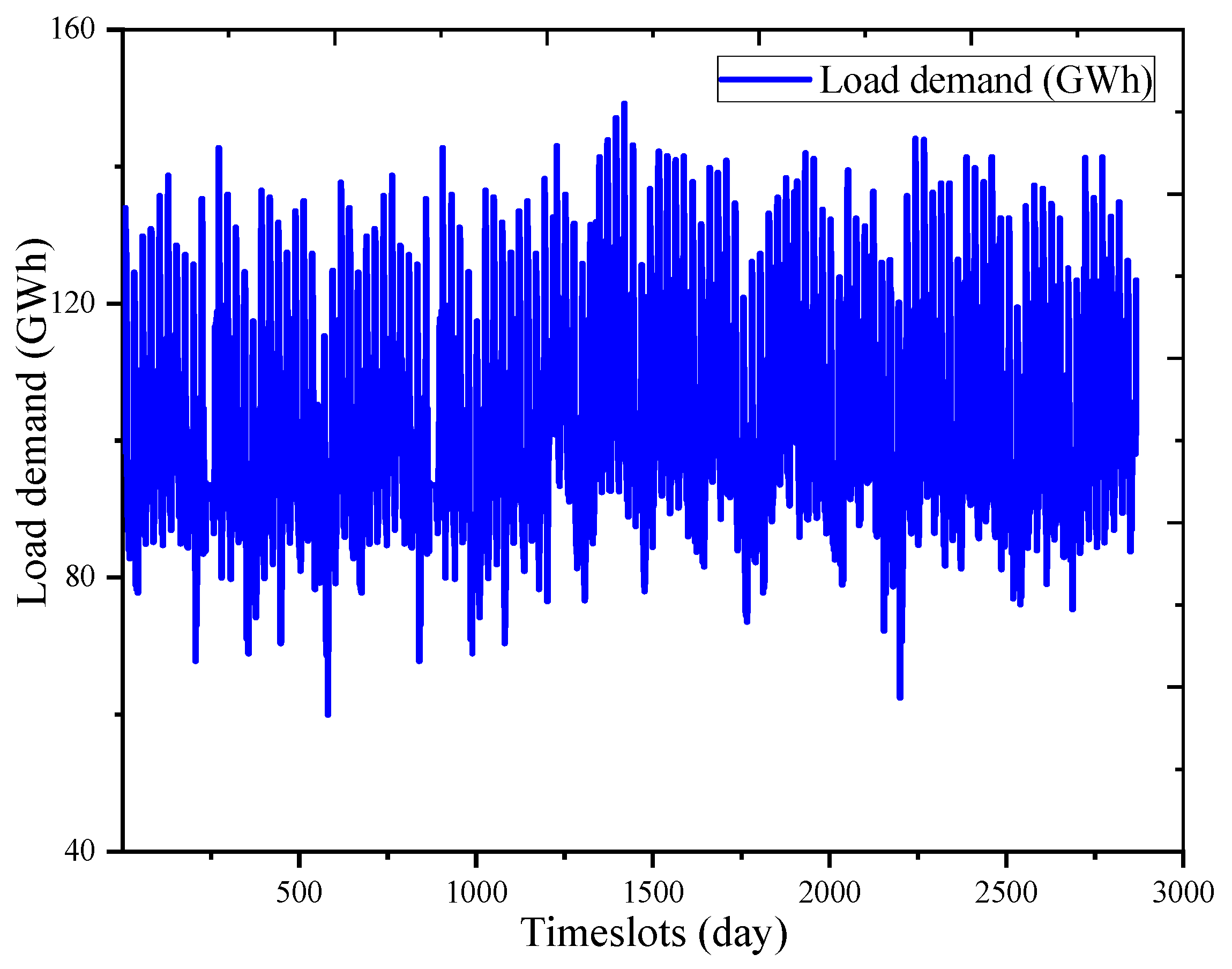
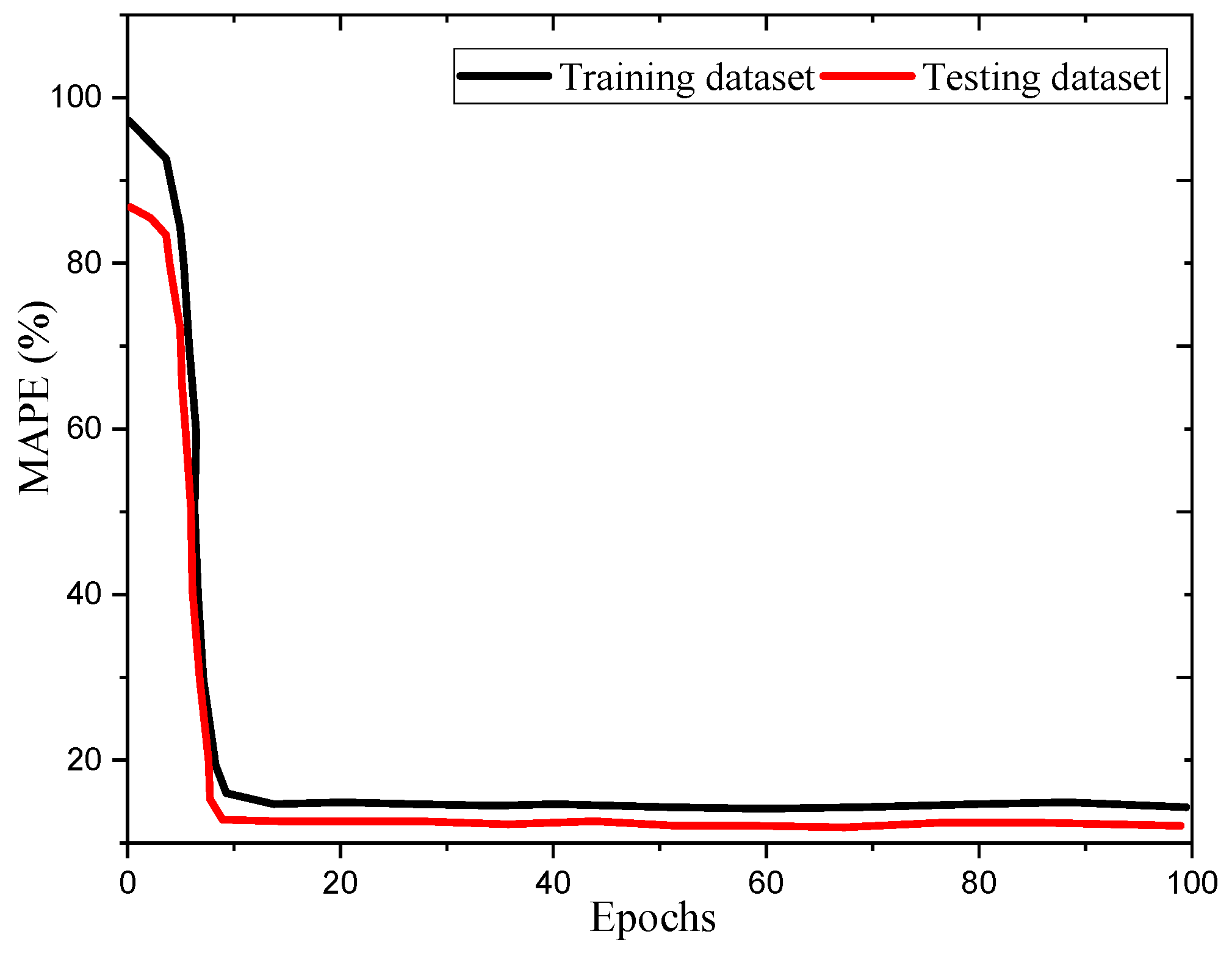
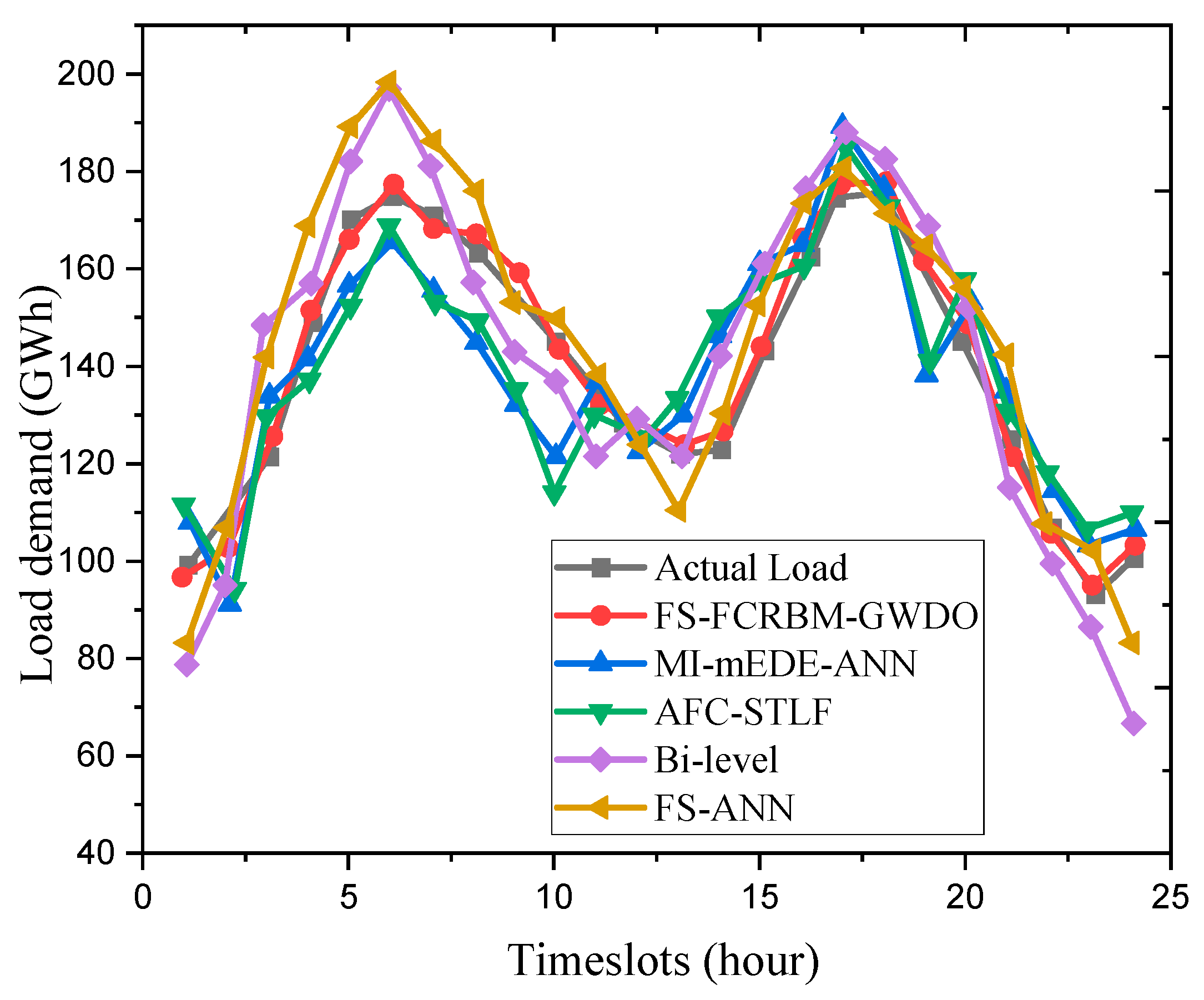
5.1. Stage One: Electrical Load Forecasting

In this stage, the effectiveness of the FS-FCRBM-GWDO framework, along with benchmark frameworks such as AFC-STLF, Bi-level, MI-mEDE-ANN, and FS-ANN, is evaluated. These benchmarks were selected due to their architectural similarities with the proposed framework. However, the FS-FCRBM-GWDO and the benchmark models have distinct computational challenges, focusing on accuracy, convergence rate, or stability. The FS-FCRBM-GWDO model was tested using real-time hourly energy usage data from the Rwandan power system, covering four years from 2018 to 2021. A total of 80% of the data was used for training the FCRBM model, while the remaining 20% was used for testing. The control parameters used in the simulations were consistent across both the proposed and benchmark models, ensuring a fair comparison. The FS-FCRBM-GWDO framework was assessed using two performance metrics: (i) accuracy, measured by the Mean Absolute Percentage Error (MAPE), variance (σ²), and Pearson correlation coefficient; and (ii) convergence speed, measured by the execution time and convergence rate. The variance (${\sigma }^2$) is mathematically represented in Equation (16), as follows:

$${\mathsf{\sigma }}^2={\displaystyle \frac{1}{\tau }}\sum _{t=1}^{\tau }\left(R_t-F_t\right),$$

(16)

The symbol $\tau$ indicates the number of timeslots, $R_t$ identifies the actual load, $F_t$ represents the predicted load at time $t$, and ${\mathsf{\sigma }}^2$ represents the variance. The accuracy of the performance metrics is computed using the following formula:

$$\mathrm{A}\mathrm{c}\mathrm{c}\mathrm{u}\mathrm{r}\mathrm{a}\mathrm{c}\mathrm{y}=100-\mathrm{M}\mathrm{A}\mathrm{P}\mathrm{E}\left(\mathrm{x}\right).$$

(17)

The convergence speed is determined by both the execution time and the convergence rate. The following is a comprehensive description:

1. Execution Time: This metric refers to the duration required for the forecasting model to predict future electrical energy consumption patterns. It is measured in seconds, with faster models having shorter execution times.

2. Convergence Rate: This aspect measures the speed at which the model reaches a specific epoch in which performance stabilizes, and the error ceases to decrease significantly with additional epochs. Models with a high convergence rate reach this stabilization point quickly, often at early epochs. Forecasting models are classified as fast if they exhibit minimal execution times and achieve early convergence, indicating efficient performance. The hourly load data is split into three datasets: training, testing, and validation, as depicted in Figure 4. The simulation parameters for the GWDO model, including the number of hidden layers, neurons, and learning rate, are presented in

Table 2. GWDO simulation parameters.

Control Parameters	Value
Number of hidden layers	1
Number of neurons in hidden layer	10
Output layer	1
Number of output neurons	1
Number of epochs	100
Number of iterations	100
Learning rate	0.0019
Momentum	0.6
Initial weight	0.1
Initial bias	0
Max	0.9
Min	0.1
Decision variables	2
Population size	24
Delay in weight	0.0002
Historical load data	4 years
Exogenous parameters	4 years

. Key parameters such as population size, historical load data, and decision variables are also outlined.

The learning evaluation process compares a model’s performance on training and testing data over multiple epochs to determine whether it is genuinely learning. A poor learning curve, with high variance and bias, indicates overfitting, while a good curve, like that of the FCRBM model, shows low variance and bias with decreasing errors. Initially, the model has a high error rate (MAPE), which decreases with more training, reaching a minimal value, indicating effective learning. Figure 5 illustrates these results.

Figure 6 provides a comparative analysis of the FS-FCRBM-GWDO framework against benchmark models like FS-ANN, AFC-STLF, Bi-level, and MI-mEDE-ANN in predicting day-ahead electrical energy consumption for the REG load data center.

Table 3. Rwanda’s January 2018 results: a comparison of the proposed and current models’ performances based on correlation coefficient, variance, and MAPE.

Electrical Load Consumption Forecasting Models
Day	FS-FCRBM-GWDO			MI-mEDE-ANN			AFC-STLF			Bi-Level			FS-ANN
	MAPE	${\mathit{\sigma }}^2$	r	MAPE	${\mathit{\sigma }}^2$	r	MAPE	${\mathit{\sigma }}^2$	r	MAPE	${\mathit{\sigma }}^2$	r	MAPE	${\mathit{\sigma }}^2$	r
1	1.13	1.19	0.70	2.20	1.55	0.50	2.30	1.60	0.52	2.60	1.69	0.50	3.41	1.87	0.50
2	1.10	0.98	0.68	2.10	1.45	0.58	2.15	1.55	0.56	2.80	1.80	0.51	3.29	1.79	0.40
3	1.09	1.10	0.71	2.50	1.30	0.51	2.10	1.48	0.53	2.75	1.51	0.39	3.18	1.73	0.29
4	1.03	0.97	0.80	2.02	1.20	0.50	2.40	1.49	0.54	2.85	1.72	0.51	3.37	1.92	0.37
5	1.50	1.09	0.65	2.10	1.15	0.55	2.25	1.37	0.55	2.87	1.59	0.34	3.20	1.81	0.40
6	1.30	1.07	0.75	2.30	1.34	0.65	2.15	1.35	0.69	2.89	1.71	0.61	3.17	1.89	0.51
7	1.24	1.04	0.69	2.11	1.55	0.60	2.10	1.60	0.65	2.75	1.70	0.32	3.71	1.94	0.40
8	1.23	1.02	0.70	2.15	1.45	0.50	2.09	1.65	0.55	2.70	1.80	0.49	3.63	1.79	0.51
9	1.08	1.05	0.80	2.35	1.36	0.55	2.50	1.66	0.56	2.65	1.62	0.62	3.56	1.84	0.42
10	1.05	0.99	0.79	2.40	1.39	0.69	2. 44	1.67	0.60	2.63	1.81	0.57	3.08	1.93	0.49
11	1.15	1.10	0.87	2.01	1.45	0.77	2.35	1.55	0.75	2.70	1.58	0.42	3.04	1.9	0.50
12	1.25	1.11	0.65	2.06	1.50	0.55	2.12	1.58	0.55	2.60	1.70	0.39	3.68	1.81	0.40
13	1.10	0.96	0.81	2.10	1.55	0.71	2.20	1.43	0.75	2.63	1.73	0.34	3.29	1.72	0.29
14	1.12	0.99	0.79	2.12	1.37	0.75	2.23	1.47	0.70	2.36	1.68	0.39	3.43	1.62	0.28
15	1.10	1.03	0.78	2.13	1.46	0.78	2.27	1.30	0.73	2.50	1.62	0.52	3.67	1.91	0.53
16	1.18	1.05	0.79	2.00	1.39	0.70	2.13	1.35	0.78	2.58	1.71	0.61	3.31	1.9	0.48
17	1.19	1.08	0.80	2.13	1.48	0.60	2.35	1.55	0.65	2.56	1.65	0.63	3.36	1.81	0.51
18	1.21	1.09	0.85	2.19	1.29	0.85	2.10	1.36	0.64	2.65	1.69	0.67	3.82	1.78	0.50
19	1.25	1.12	0.90	2.16	1.36	0.50	2.14	1.55	0.59	2.54	1.64	0.62	3.44	1.69	0.39
20	1.44	0.95	0.67	2.17	1.47	0.60	2.15	1.45	0.48	2.50	1.59	0.61	3.16	1.72	0.54
21	1.39	0.90	0.71	2.34	1.51	0.58	2.19	1.54	0.58	2.59	1.80	0.53	3.31	1.91	0.43
22	1.17	0.99	0.75	2.10	1.50	0.75	2.10	1.40	0.59	2.80	1.58	0.50	3.51	1.73	0.41
23	1.15	1.01	0.86	2.30	1.45	0.64	2.13	1.34	0.39	2.75	1.71	0.61	3.35	1.72	0.52
24	1.08	1.07	0.87	2.01	1.34	0.73	2.24	1.60	0.58	2.65	1.63	0.39	3.92	1.81	0.41
25	1.03	1.11	0.92	1.99	1.35	0.82	2.13	1.49	0.67	2.67	1.53	0.61	3.89	1.8	0.39
26	1.05	1.05	0.90	2.00	1.56	0.09	2.26	1.61	0.49	2.85	1.70	0.68	3.75	1.59	0.52
27	1.03	1.10	0.88	2.10	1.40	0.58	2.10	1.48	0.77	2.55	1.75	0.62	3.79	1.79	0.49
28	1.25	1.11	0.76	2.09	1.35	0.56	2.15	1.50	0.58	2.60	1.75	0.55	3.35	1.81	0.38
29	1.27	1.13	0.77	2.08	1.32	0.55	2.13	1.53	0.59	2.62	1.76	0.49	3.36	1.78	0.39
30	1.25	1.21	0.81	2.01	1.21	0.43	2.21	1.48	0.51	2.58	1.69	0.51	3.34	1.74	0.36
Agg.	1.10	1.03	0.79	2.20	1.25	0.65	2.10	1.35	0.60	2.6	1.70	0.52	3.4	1.80	0.43

further details the accuracy of these models, comparing metrics such as the Mean Absolute Percentage Error (MAPE), variance, and correlation coefficient. The findings clearly indicate that the FS-FCRBM-GWDO architecture offers superior accuracy in forecasting the next day’s electrical energy consumption for Rwanda’s power system. Both the proposed and the benchmark models are adept at capturing and adapting to the non-linear patterns present in historical energy consumption time series data.

The proposed hybrid FS-FCRBM-GWDO model uses nonlinear activation functions like tangent hyperbolic (tanh), sigmoid, and ReLU to predict energy consumption patterns. Unlike benchmark frameworks like FS-ANN, AFC-STLF, Bi-level, and MI-mEDE-ANN, which use sigmoid activation functions, the proposed model uses ReLU and multivariate autoregressive algorithms for rapid convergence and addressing vanishing gradient and overfitting issues. The model’s energy consumption pattern closely aligns with actual data, with a MAPE of 1.10%, outperforming the standard frameworks with values of 2.2%, 2.1%, 3.4%, and 2.6%, respectively. Hence, the results presented in Figure 6 and Table 3 suggest that the hybrid FS-FCRBM-GWDO model outperforms the standard frameworks in terms of accuracy.

Figure 7 shows a week-long prediction of the hourly electrical energy consumption, demonstrating the superior performance of the FS-FCRBM-GWDO model compared to existing models like FS-ANN, AFC-STLF, Bi-level, and MI-mEDE-ANN. The FS-FCRBM-GWDO model achieved a MAPE of 1.18%, significantly outperforming the benchmark models. The model’s accuracy is attributed to the use of a deep-learning-based FCRBM with ReLU, a multivariate autoregressive algorithm, and GWDO optimization. Figure 8 and Table 3 show that the FS-FCRBM-GWDO model closely tracks the actual energy consumption curve, ensuring better performance in monthly predictions.

Table 4. Rwanda’s results for the year 2018: comparative performance analysis of the FS-FCRBM-GWDO and existing models in terms of MAPE, correlation coefficient, and variance.

Electrical Load Consumption Forecasting Models
Month	FS-FCRBM-GWDO			MI-mEDE-ANN			AFC-STLF			Bi-Level			FS-ANN
	MAPE	${\mathit{\sigma }}^2$	r	MAPE	${\mathit{\sigma }}^2$	r	MAPE	${\mathit{\sigma }}^2$	r	MAPE	${\mathit{\sigma }}^2$	r	MAPE	${\mathit{\sigma }}^2$	r
1	1.09	1.12	0.81	2.22	1.38	0.81	2.3	1.28	0.69	2.49	1.61	0.39	3.61	1.9	0.49
2	1.37	1.01	0.7	2.09	1.5	0.58	2.09	1.51	0.51	2.48	1.59	0.61	3.19	1.59	0.51
3	1.32	1.20	0.59	2.1	1.47	0.62	2.2	1.6	0.49	2.59	1.7	0.5	3.64	1.82	0.29
4	1.12	0.89	0.77	1.99	1.19	0.43	2.35	1.52	0.6	2.9	1.81	0.38	3.32	1.78	0.4
5	1.28	1.12	0.68	2.21	1.5	0.54	2.29	1.6	0.58	2.62	1.69	0.6	3.37	1.83	0.48
6	1.09	1.11	0.92	2.29	1.38	0.59	2.08	1.28	0.42	2.68	1.72	0.62	3.17	1.69	0.52
7	1.1	1.20	0.58	2.07	1.6	0.57	2.03	1.57	0.7	2.69	1.57	0.38	3.73	1.78	0.41
8	1.18	1.07	0.69	2.04	1.39	0.43	2.11	1.59	0.6	2.95	1.8	0.62	3.61	1.91	0.39
9	1.3	1.09	0.62	2.1	1.46	0.62	2.21	1.61	0.49	2.54	1.6	0.34	3.6	1.64	0.41
10	1.09	1.10	0.81	2.05	1.42	0.68	2.08	1.42	0.8	2.59	1.79	0.61	3.18	1.93	0.53
11	1.08	1.06	0.92	2.07	1.56	0.82	2.29	1.64	0.72	2.63	1.8	0.29	3.09	1.79	0.5
12	1.15	1.15	0.79	2.3	1.32	0.91	2.09	1.45	0.7	2.72	1.69	0.63	3.85	1.93	0.51
Agg.	1.18	1.09	0.74	2.12	1.43	0.63	2.17	1.50	0.60	2.65	1.69	0.50	3.45	1.80	0.45

presents a performance evaluation for the leap year of 2018, using MAPE, variance, and correlation coefficient metrics.

FS-FCRBM-GWDO module’s performance in terms of MAPE and convergence speed.

Figure 9, Figure 10 and Figure 11 present a statistical assessment of MAPE, execution time, and convergence speed for the proposed FS-FCRBM-GWDO model and benchmark models (FS-ANN, AFC-STLF, MI-mEDE-ANN, and Bi-level). The FS-FCRBM-GWDO model achieved the lowest MAPE of 1.18%, indicating high accuracy, compared to higher MAPE values in the benchmark models of 3.45%, 2.17%, 2.12%, and 2.65%, respectively. However, integrating the optimization module increases the execution time from 25 to 95 s. The FS-FCRBM-GWDO model balances accuracy and speed by using GWDO for optimization, ReLU activation, a multivariate autoregressive algorithm, the deep learning FCRBM, and advanced data preprocessing. Despite longer execution times compared to FS-ANN, the FS-FCRBM-GWDO model offers superior accuracy and efficiency.

Figure 11 illustrates the convergence speed of the proposed hybrid FS-FCRBM-GWDO model compared to benchmark models, including FS-ANN, Bi-level, AFC-STLF, and MI-mEDE-ANN, based on 100 iterations. As the number of iterations increases, the MAPE decreases for all the models. Notably, the proposed model demonstrates rapid convergence, reaching stability around the 10th iteration, indicating its efficient search ability. In contrast, benchmark models such as FS-ANN, Bi-level, AFC-STLF, and MI-mEDE-ANN converge later, around the 33rd, 29th, 25th, and 21st iterations, respectively, showcasing slower convergence rates. This analysis suggests that the proposed GWDO algorithm offers superior performance for optimization in integrated frameworks due to its faster convergence compared to existing benchmark models. The convergence analysis focuses solely on the MAPE performance metric for both proposed and existing models.

Figure 12 compares the proposed hybrid FS-FCRBM-GWDO model to benchmark models, including FS-ANN, Bi-level, AFC-STLF, and MI-mEDE-ANN, regarding the cumulative distribution function (CDF) of error. The FS-FCRBM-GWDO model outperforms the current models in terms of CDF. The FCRBM model, which utilizes deep learning, is capable of providing accurate predictions even in situations characterized by high levels of uncertainty. This is due to the deep layers of the model being able to effectively capture the essential characteristics. Therefore, our suggested FS-FCRBM-GWDO framework is a superior option for distribution system operators to achieve efficient and effective energy management for the smart grid. The FS-FCRBM-GWDO framework, along with other current frameworks, like FS-ANN, Bi-level, AFC-ANN, and MI-mEDE-ANN, was evaluated in terms of computational complexity, execution time, convergence rate, and accuracy.

A further evaluation of the FS-FCRBM-GWDO framework and existing frameworks, such as FS-ANN, Bi-level, AFC-ANN, and MI-mEDE-ANN, is presented in

Table 5. Evaluation of the proposed and benchmark models in terms of computational complexity, execution time, convergence rate, and accuracy.

Performance Parameters	Models
	FS-ANN	Bi-Level	AFC-STLF	MI-mEDE-ANN	FS-FCRBM-GWDO
Computational complexity (level)	Low	High	Moderate	High	Moderate
Convergence rate (epochs)	33rd	28th	26th	21st	11th
Execution time (s)	31	89	62	97.5	98.9
Accuracy (%)	96.4	97.4	97.9	97.8	98.7

. This evaluation encompasses computational complexity, execution time, convergence rate, and accuracy metrics. Based on the simulation results, performance analysis, and discussions, it is concluded that the proposed hybrid FS-FCRBM-GWDO model surpasses benchmark models in terms of convergence rate, accuracy, computational complexity, and execution time.

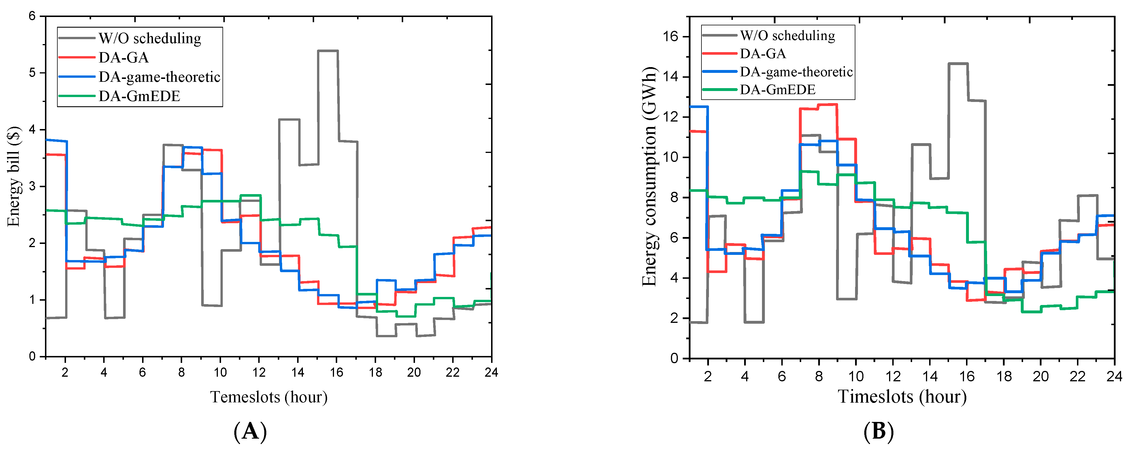
5.2. Energy Management Based on the DA-GmEDE Framework

This study presents the results of a DA-GmEDE-based energy management strategy for residential buildings with three types of appliances: time-shiftable, power-shiftable, and critical appliances. The system module and the GmEDE-based solution are used to validate the performance of the strategy, which uses a day-ahead demand response price signal and energy consumption forecast generated using ANN. The scheduling time horizon spans 24 h, and the ANN is trained to forecast DR prices, which the Energy Management Controller (EMC) uses to optimize appliance scheduling. The parameters of the algorithms employed in the simulations, as well as descriptions of all the residential appliances, are detailed in

Table 6. Parameters used in simulation for the proposed and existing energy management strategies.

Parameters	Values
Population	100
Minimum lower population bound	0.1
Maximum lower population bound	0.9
Number of wolves in each pack	17
Maximum epochs	100
Decision variables	2
Learning rate	0.002
Weight decay	0.0002
Initial value of weight	0.1
Initial value of bias	0
Number of objectives	2
Momentum	0.5
Feature selection threshold	0.5
Distance from prey	Vary
Status of leader	1 or 2
Number of dimensions	17
Gradient of problem	Vary

and

Table 7. Parameters of residential home appliances used in simulations.

Classification	Types of Application	Power Rating (GWh)	Operation Timeslots (h)	Priority
Power-shiftable appliances	Electric radiator	(0.5–1.5)	10	2
	Water dispenser	(0.8–1.2)	24
	Refrigerator	(0.5–1.2)	24
	Air conditioner	(0.8–1.5)	10
Critical appliances	Hair dryer	1.2	1	3
	Microwave	1.8	3
	Electric iron	1.8	4
	Electrical kettle	1.5	1
Time shiftable Appliances	Washing machine	0.7	5	1
	Cloth dryer	2	4
	Water pump	0.4	2

Table 7 classifies residential appliances into power-shiftable, critical, and time-shiftable categories, with each assigned a priority based on their importance. Critical appliances, like the hair dryer (priority 3), are given precedence in energy management, while time-shiftable appliances, such as the washing machine (priority 1), can be operated during low-demand periods to optimize energy usage. Power-shiftable appliances, like the electric radiator (priority 2), balance energy efficiency and comfort.

, respectively.

The proposed method, based on the EMC, is compared to current techniques like the Day-Ahead Genetic Algorithm (DA-GA) and DA-game-theoretic. The proposed scheduling approach, DA-GmEDE, is compared to the W/O, DA-GA, and DA-game-theoretic strategies. The efficacy of the proposed method is evaluated using electricity cost, PAR, and user discomfort balance.

Figure 13A,B illustrates the predicted pricing signal and energy use patterns for the upcoming day.

5.3. Energy Consumption and Corresponding Electricity Bills across Four Different Modes of Operation

The DA-GmEDE method calculates energy consumption and electricity cost profiles for four operational modes. It shows that residential structures’ energy consumption is higher under mode IV compared to modes I and III but lower than mode II within the scheduling time horizon. The peak energy consumption is significantly lower in mode II, which is attributed to customers prioritizing comfort and continuing activities despite higher costs. These profiles are represented in Figure 14A,B.

Consumers in operation mode III consume more energy, but less than in mode II and IV due to their prioritizing of PAR. Mode I customers have lower energy usage but prioritize reducing electricity expenses. The EMC, based on DA-GmEDE, allows customers to meet their needs in various operational modes, resulting in lower electricity bills.

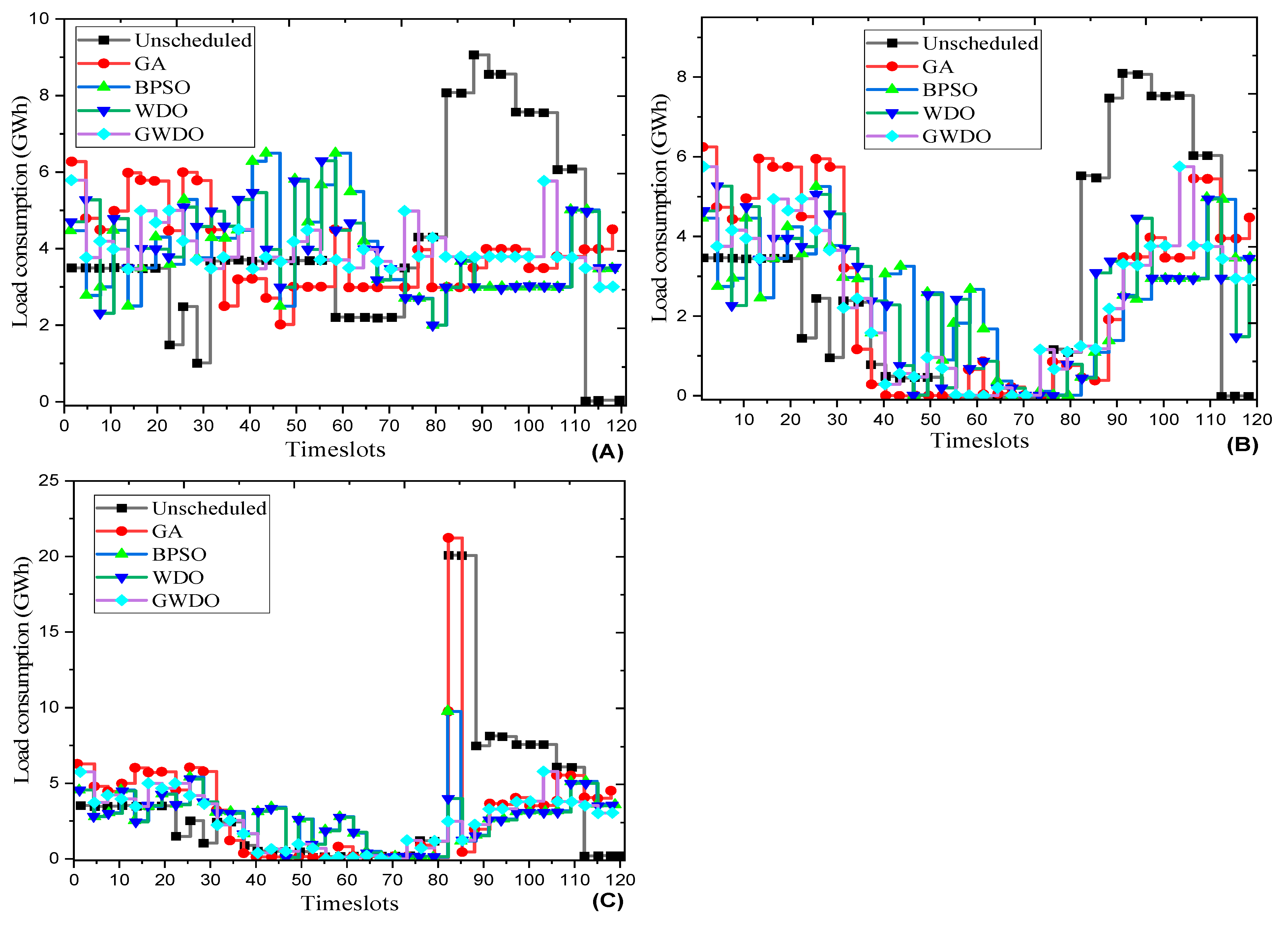
5.4. Energy Consumption of Residential Buildings within the Scheduling Time Horizon

Figure 15A,B shows energy consumption patterns in a home without and after scheduling with the DA-GA, DA-game-theoretic, and proposed DA-GmEDE strategies. In the absence of scheduling, energy consumption peaks during peak demand hours, leading to high electricity bills and a high Peak-to-Average Ratio. After scheduling with these strategies, energy consumption was significantly reduced. The proposed DA-GmEDE strategy achieves a 36.4% improvement over the W/O scheduling case and a 33.3% improvement over both strategies, demonstrating its ability to generate the most suitable load profile for residential buildings.

5.5. Electricity Bill per Hour for a Home in a Residential Building within the Scheduling Time Horizon

Figure 15B demonstrates the effectiveness of scheduling methods like DA-GmEDE, DA-GA, DA-game-theoretic, and W/O scheduling in reducing electricity bills. Prior to scheduling, peak periods led to increased costs, resulting in a surge of up to USD 5.5. By implementing these methods, electricity costs per timeslot were decreased by USD 0.7, USD 1.2, and USD 0.9, respectively. The DA-GmEDE-based approach outperforms other strategies by 41.6% and 22.2%.

The evaluation of the Peak-to-Average Ratio (PAR) is presented, comparing without-scheduling and scheduling conditions using DA-GA, DA-game-theoretic, and DA-GmEDE strategies. The proposed DA-GmEDE-based strategy outperforms other strategies in terms of PAR. Figure 16A demonstrates its effectiveness in maintaining balanced energy consumption and improving power system stability. The EMCs effectively shift the load under day-ahead pricing signals, reducing the PAR by 17.64%, 25.49%, and 47.05%, respectively. Figure 16B evaluates the total electricity bill payments using DA-GA, DA-game-theoretic, and DA-GmEDE strategies. The proposed DA-GmEDE strategy achieves the highest reduction in bills, outperforming existing strategies and demonstrating effectiveness in reducing overall electricity expenses by 15.2%, 8.7%, and 23.9%, respectively.

6. Performance Tradeoff Analysis

Figure 17 shows the performance tradeoff between the proposed DA-GmEDE strategy and existing strategies (DA-GA and DA-game-theoretic) in terms of electricity bills and waiting times. The proposed DA-GmEDE strategy minimizes the tradeoff between electricity bills and waiting times, making it a favorable choice for energy management tasks. This balance between electricity bills and user discomfort is more pronounced for DA-GA- and DA-game-theoretic-based strategies.

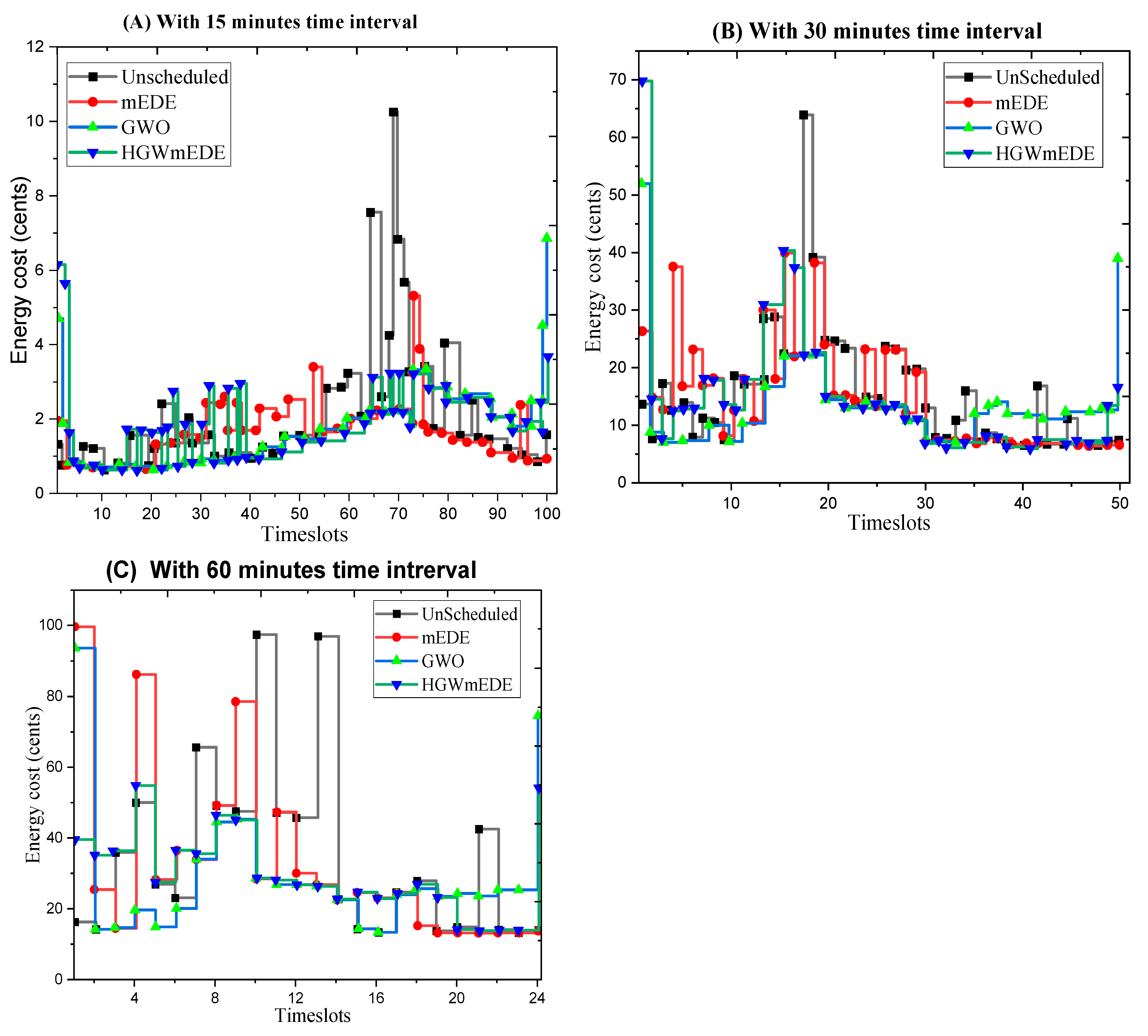
6.1. Electricity Cost Evaluation under a Price-Based DR Program

To assess the cost parameters of the suggested plan, simulations were run with several Operating Time Interval (OTI) lengths, specifically 15, 30, and 60 min. The proposed framework to compute power costs utilizes the daily energy pricing signals, obtained from the Rwanda Utility Regulatory Authority (RURA). The National Control Center (NCC) provides real-time pricing signals (RTPSs) and critical peak pricing signals (CPPSs).

6.2. Electricity Cost Evaluation Using RTPS and CPPS under OTI

By scheduling smart home appliances using anticipated RTPSs, the proposed GmEDE algorithm efficiently reduces electricity costs when compared to modified Evolutionary Differential Evolution (mEDE) and Grey Wolf Optimization (GWO). The program optimizes the transition of appliances from on-peak to off-peak timeslots by coordinating pricing schemes with patterns of energy use. The suggested GmEDE-based expenses reduce demand peaks and energy prices compared to both GWO and mEDE. The simulations demonstrate that by arranging smart home equipment in the best possible way, the suggested GmEDE algorithm continuously lowers power bills.

The proposed GmEDE-based framework outperforms both GWO and mEDE in terms of reducing peaks in demand and electricity costs. Figure 18A shows that unscheduled loads result in high demand peaks, resulting in high prices during specific hours. Figure 18B shows that GWO presents higher costs at the beginning timeslots, while GmEDE maintains minimum costs throughout the 24 h. Figure 18C shows that the proposed GmEDE algorithm consistently reduces electricity costs by optimally scheduling smart home appliances.

The electricity cost profile for a 15-min OTI shows that the forecast CPPS remains constant, except during critical peak hours. The maximum peak in an unscheduled load scenario is USD 1.8155, but when smart home appliances are scheduled, it reduces to USD 0.8307. The 30-min OTI has similar costs, but no peaks emerge, except at the starting time of the day. The proposed GmEDE algorithm significantly reduces the unscheduled appliance electricity cost from USD 7.668 to USD 2.0346 for the 60-min OTI as highlighted in Figure 19A–C. The overall unscheduled cost is reduced from USD 13.00891 to USD 10.8591 when smart home appliances are scheduled using the GmEDE algorithm.

In Figure 20 and Figure 21, the results analysis shows that the proposed GWDO algorithm outperforms other heuristic techniques (GA, BPSO, and WDO) and unscheduled loads in optimizing energy consumption and reducing electricity costs. Without RESs and ESS, GWDO reduces peak power consumption by 35.16% compared to 32.96% for GA, 31.86% for BPSO, and 33.51% for WDO. With RESs, GWDO achieves a 28.39% reduction in peak power consumption, outperforming GA (24.69%), BPSO (30.86%), and WDO (32%). Additionally, GWDO provides the lowest electricity costs, peaking at USD 0.0049/kWh compared to GA (USD 0.009 cents/kWh), BPSO (USD 0.006/kWh), and WDO (USD 0.0055/kWh), demonstrating the most stable and optimal profiles across the scenarios.

Additionally, the overall electricity cost reduction for 30 and 60 min OTIs is depicted in Figure 22. A brief comparison of electricity costs under forecasted RTPS and CPPS for 15, 30, and 60 min OTIs is provided in

Table 8. Overall electricity cost comparative evaluation for 24 h time horizon under forecast RTPS and CPPS.

Scenarios and Algorithms	Electrical Energy Cost (USD) under RTPS			Electrical Energy Cost (USD) under CPPS
	15 min	30 min	60 min	15 min	30 min	60 min
Without scheduling	500.4821	743.4871	822.1561	1200.1561	1300.8910	1085.6481
GWO	426.0507	727.1431	717.9402	1190.5122	1200.9612	1080.4091
mEDE	420.5381	743.1951	831.2132	1178.4901	1164.4901	1190.6901
GmEDE	416.7468	658.6502	712.7292	1164.4901	1085.9022	1056.7891

. In summary, the proposed framework optimally schedules smart home appliances, leading to reduced overall aggregated electricity costs for residents compared to mEDE and GWO under forecasted RTPS and CPPS.

6.3. Peaks in Demand

Peaks in demand are the highest loads experienced within a 24-h period, representing maximum energy consumption. To minimize these peaks, Demand Side Management strategies like peak clipping, load shifting, and price-based demand response can be implemented. These strategies reduce peaks in demand, electricity costs, and strain on energy-user consumers. The subsequent section evaluates the effectiveness of peak reduction strategies in both real-time pricing schemes (RTPSs) and critical peak pricing schemes (CPPSs). Figure 23 shows the decrease in the demand peaks under RTPS for various OTIs. Peak demand occurs when the load is not scheduled, while when scheduled using mEDE and GWO, the peak demand values are 8.1723 and 5.6750, respectively. The proposed GmEDE scheme achieves a 53.02% decrease in peaks, demonstrating superior performance compared to the GWO and mEDE schemes, resulting in reductions of 25.50% and 48.26%, respectively, as illustrated in

Table 9. Peaks in demand evaluation for the proposed and existing schemes for 24 h.

Scenarios	Peak Load in Demand under RTPS with Different OTIs			Peak Load in Demand under CPPS with Different OTIs
	15 min	30 min	60 min	15 min	30 min	60 min
Without scheduling	10.9698	6.0258	5.0258	10.9698	5.8035	5.0258
mEDE	8.1723	5.8425	3.6558	8.1723	5.2537	3.8425
GWO	5.676	5.9336	4.3509	5.6265	4.8166	3.9336
GmEDE	5.1531	3.6210	2.5369	5.5416	4.0264	3.6210

.

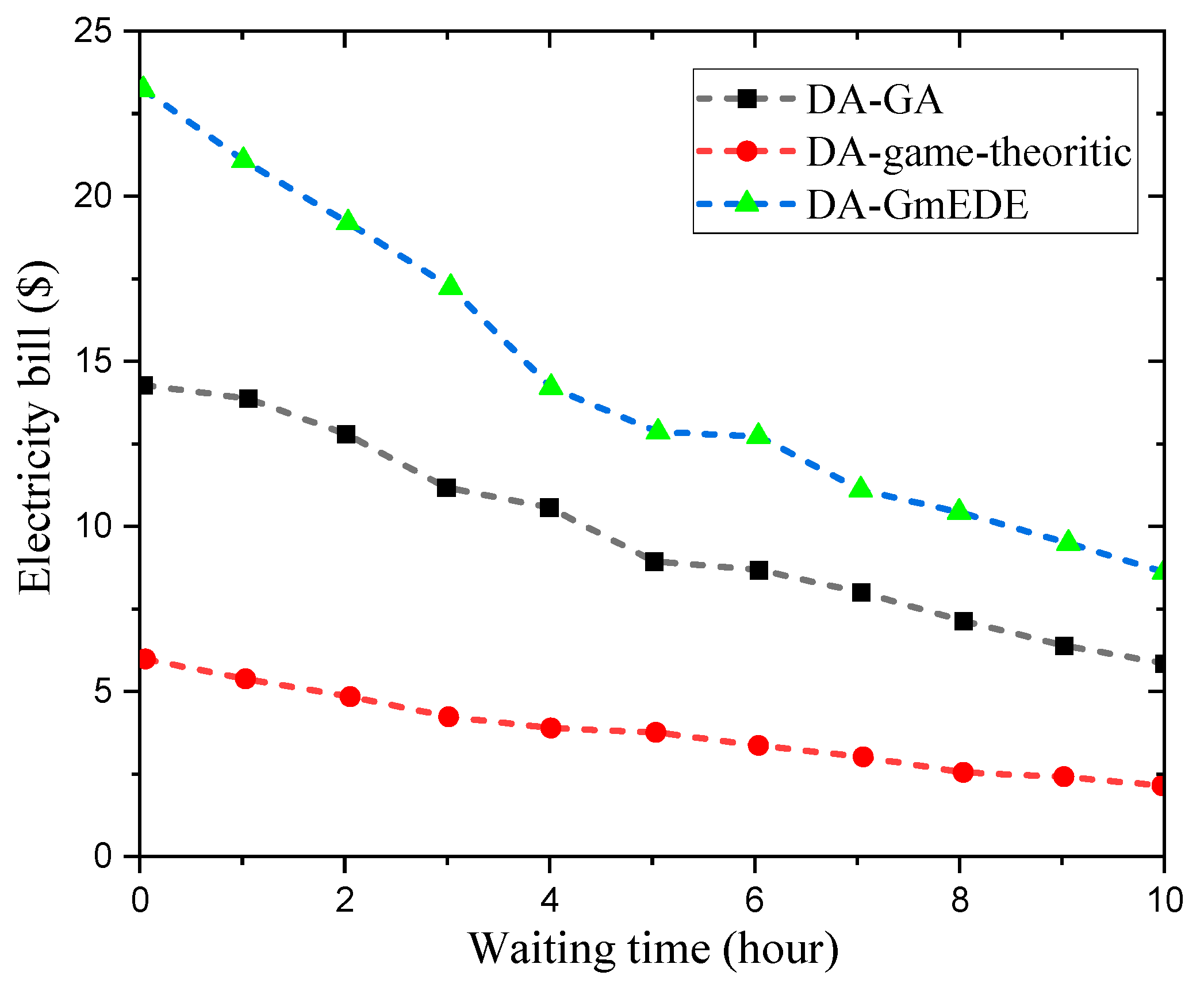
6.4. Waiting Time Evaluation

Figure 24 depicts the waiting times for the planned GmEDE and the existing mEDE and GWO under CPPS. The measured waiting times for mEDE, GWO, and the proposed GmEDE are 3.39 h, 4.23 h, and 6.49 h, respectively. The load plan generated by the EMC using the GmEDE algorithm clearly exhibits longer waiting times, suggesting that user comfort is sacrificed in order to reduce electricity expenses.

Table 10. Comparative evaluation of the proposed GmEDE and existing (mEDE and GWO) algorithm in terms of waiting time under RTPS and CPPS for different OTIs.

Scenarios	Evaluation of Waiting under RTPS for Different OTI			Evaluation of Waiting under CPPS for Different OTI
	15 min	30 min	60 min	15 min	30 min	60 min
mEDE	4.3781 h	4.5394 h	2.6560 h	3.3826 h	4.8012 h	2.8158 h
GWO	9.7494 h	10.0262 h	2.2397 h	4.2293 h	5.7853 h	3.3346 h
GmEDE	10.4249 h	12.7007 h	3.8793 h	6.4814 h	6.1335 h	4.3408 h

presents a statistical analysis of the proposed and current algorithms, specifically in terms of waiting times, for different OTIs under RTPS and CPPS.

7. Conclusions

In this research, a novel hybrid model, FS-FCRBM-GWDO, is proposed for forecasting electrical energy consumption, aiming to deliver accurate predictions while maintaining a reasonable convergence rate. First, the model integrates feature selection (FS) with a forecaster based on the Factored Conditional Restricted Boltzmann Machine (FCRBM), allowing for more precise predictions by selecting key features using relevancy and redundancy filters from the Mutual Information (MI) approach. Second, the Genetic Wind-Driven Optimization (GWDO) algorithm is introduced to optimize the forecasting process, enhancing both accuracy and convergence in handling nonlinear and complex patterns of energy consumption. To validate its effectiveness, the FS-FCRBM-GWDO model was tested using data from the Rwanda power grid, and it achieved an accuracy of 98.9%, outperforming benchmark models such as MI-mEDE-ANN, AFC-STLF, Bi-level, and FS-ANN. Notable improvements were also observed in reducing the average execution time. Thirdly, this research also presents a strategy for effective energy management through an Energy Management Control (EMC) framework supported by a Day-Ahead Genetic Modified Evolutionary Differential Evolution (DA-GmEDE) strategy. This approach optimizes energy consumption by scheduling household appliances, reducing power costs, and improving the Peak-to-Average Ratio (PAR), thereby enhancing power system stability. The DA-GmEDE-based strategy demonstrated superior reductions in both electricity bills and PAR compared to alternative methods. Finally, the study introduces a modular architecture utilizing the GmEDE algorithm, which leverages predicted energy consumption patterns to optimize load scheduling for both users and energy providers. By smoothing the demand curve and lowering electricity costs, this approach benefits households and improves grid stability. The GWDO algorithm, combining elements of GA and WDO, further reduces electricity costs and PAR in scenarios involving renewable energy sources and energy storage systems, outperforming other methods and emphasizing the significance of accurate energy consumption forecasting for efficient smart grid management. Future research could further enhance the accuracy, scalability, and applicability of energy consumption forecasting models in various energy environments and smart grid infrastructures.

References

1. Giamarelos, N.; Papadimitrakis, M.; Stogiannos, M.; Zois, E.N.; Livanos, N.-A.I.; Alexandridis, A. A Machine Learning Model Ensemble for Mixed Power Load Forecasting across Multiple Time Horizons. Sensors 2023, 23, 5436. [Google Scholar] [CrossRef]
2. Zhao, W.; Fan, L. Short-Term Load Forecasting Method for Industrial Buildings Based on Signal Decomposition and Composite Prediction Model. Sustainability 2024, 16, 2522. [Google Scholar] [CrossRef]
3. Xin, F.; Yang, X.; Beibei, W.; Ruilin, X.; Fei, M.; Jianyong, Z. Research on electric vehicle charging load prediction method based on spectral clustering and Deep Learning Network. Front. Energy Res. 2024, 12, 1294453. [Google Scholar] [CrossRef]
4. Veeramsetty, V.; Chandra, D.R.; Grimaccia, F.; Mussetta, M. Short-term electric power load forecasting using principal component analysis and recurrent neural networks. Forecasting 2022, 4, 149–164. [Google Scholar] [CrossRef]
5. Guo, X.; Gao, Y.; Li, Y.; Zheng, D.; Shan, D. Short-term household load forecasting based on long- and short-term time-series network. Energy Rep. 2021, 7, 58–64. [Google Scholar] [CrossRef]
6. Li, D.; Liu, Q.; Feng, D.; Chen, Z. A Medium- and Long-Term Residential Load Forecasting Method Based on Discrete Cosine Transform-FED former. Energies 2024, 17, 3676. [Google Scholar] [CrossRef]
7. Panigrahi, R.; Patne, N.R.; Pemmada, S.; Manchalwar, A.D. Regression model-based hourly aggregated electricity demand prediction. Energy Rep. 2022, 8, 16–24. [Google Scholar] [CrossRef]
8. Hassnain, S.; Asar, A.; Mahmood, F. Performance of STLF model from the PSO, Time Series and regression perspectives. In Proceedings of the 2009 International Joint Conference on Neural Networks, Atlanta, GA, USA, 14–19 June 2009. [Google Scholar] [CrossRef]
9. Harun, M.H.; Othman, M.M.; Musirin, I. Short-term load forecasting (STLF) using artificial neural network based multiple lags of Time Series. Adv. Neuro-Inf. Process. 2009, 5507, 445–452. [Google Scholar] [CrossRef]
10. Zhu, K.; Geng, J.; Wang, K. A hybrid prediction model based on pattern sequence-based matching method and extreme gradient boosting for holiday load forecasting. Electr. Power Syst. Res. 2021, 190, 106841. [Google Scholar] [CrossRef]
11. Al-Ani, B.R.K.; Erkan, E.T. A study of load demand forecasting models in electricity using artificial neural networks and Fuzzy Logic Model. Int. J. Eng. 2022, 35, 1111–1118. [Google Scholar] [CrossRef]
12. Uwimana, E.; Zhou, Y.; Zhang, M. Long-term electrical load forecasting in Rwanda based on support vector machine enhanced with Q-SVM optimization kernel function. J. Power Energy Eng. 2023, 11, 32–54. [Google Scholar] [CrossRef]
13. Kaskouras, C.D.; Krommydas, K.F.; Baltas, I.; Papaioannou, G.P.; Papayiannis, G.I.; Yannacopoulos, A.N. Assessing the Flexibility of Power Systems through Neural Networks: A Study of the Hellenic Transmission System. Sustainability 2024, 16, 5987. [Google Scholar] [CrossRef]
14. Reppert, T. Local-level ownership of electricity grids: An analysis of Germany’s Distribution System Operators (DSOs). Util. Policy 2023, 85, 101678. [Google Scholar] [CrossRef]
15. Anees, A.; Chen, Y.-P.P. True real-time pricing and combined power scheduling of electric appliances in Residential Energy Management System. Appl. Energy 2016, 165, 592–600. [Google Scholar] [CrossRef]
16. Mujeeb, S.; Javaid, N.; Ilahi, M.; Wadud, Z.; Ishmanov, F.; Afzal, M.K. Deep Long Short-term memory: A new price and load forecasting scheme for big data in Smart Cities. Sustainability 2019, 11, 987. [Google Scholar] [CrossRef]
17. Deng, B.; Peng, D.; Zhang, H.; Qian, Y. An intelligent hybrid short-term load forecasting model optimized by switching delayed PSO of micro-grids. J. Renew. Sustain. Energy 2018, 10, 024901. [Google Scholar] [CrossRef]
18. Cecati, C.; Kolbusz, J.; Rozycki, P.; Siano, P.; Wilamowski, B.M. A novel RBF Training Algorithm for short-term Electric Load Forecasting and comparative studies. IEEE Trans. Ind. Electron. 2015, 62, 6519–6529. [Google Scholar] [CrossRef]
19. Ahmad, A.; Javaid, N.; Guizani, M.; Alrajeh, N.; Khan, Z.A. An accurate and fast converging short-term load forecasting model for industrial applications in a smart grid. IEEE Trans. Ind. Inform. 2017, 13, 2587–2596. [Google Scholar] [CrossRef]
20. Cai, M.; Pipattanasomporn, M.; Rahman, S. Day-ahead building-level load forecasts using deep learning vs. traditional time-series techniques. Appl. Energy 2019, 236, 1078–1088. [Google Scholar] [CrossRef]
21. Mujeeb, S.; Alghamdi, T.A.; Ullah, S.; Fatima, A.; Javaid, N.; Saba, T. Exploiting deep learning for wind power forecasting based on Big Data Analytics. Appl. Sci. 2019, 9, 4417. [Google Scholar] [CrossRef]
22. Mocanu, E.; Nguyen, P.H.; Gibescu, M.; Kling, W.L. Deep Learning for Estimating Building Energy Consumption. Sustain. Energy Grids Netw. 2016, 6, 91–99. [Google Scholar] [CrossRef]
23. Gao, Y.; Matsunami, Y.; Miyata, S.; Akashi, Y. Operational optimization for off-grid renewable building energy system using Deep Reinforcement Learning. Appl. Energy 2022, 325, 119783. [Google Scholar] [CrossRef]
24. Dedinec, A.; Filiposka, S.; Dedinec, A.; Kocarev, L. Deep belief network based electricity load forecasting: An analysis of Macedonian case. Energy 2016, 115, 1688–1700. [Google Scholar] [CrossRef]
25. Fan, C.; Xiao, F.; Zhao, Y. A short-term building cooling load prediction method using deep learning algorithms. Appl. Energy 2017, 195, 222–233. [Google Scholar] [CrossRef]
26. Amjady, N.; Keynia, F. Application of a new hybrid neuro-evolutionary system for day-ahead price forecasting of electricity markets. Appl. Soft Comput. 2010, 10, 784–792. [Google Scholar] [CrossRef]
27. Amjady, N.; Keynia, F.; Zareipour, H. Short-term load forecast of microgrids by a new bilevel prediction strategy. IEEE Trans. Smart Grid 2010, 1, 286–294. [Google Scholar] [CrossRef]
28. Liu, D.; Zeng, L.; Li, C.; Ma, K.; Chen, Y.; Cao, Y. A distributed short-term load forecasting method based on local weather information. IEEE Syst. J. 2018, 12, 208–215. [Google Scholar] [CrossRef]
29. Hafeez, G.; Alimgeer, K.S.; Wadud, Z.; Shafiq, Z.; Ali Khan, M.U.; Khan, I.; Khan, F.A.; Derhab, A. A novel accurate and fast converging deep learning-based model for electrical energy consumption forecasting in a smart grid. Energies 2020, 13, 2244. [Google Scholar] [CrossRef]
30. Shi, H.; Xu, M.; Li, R. Deep learning for household load forecasting—A novel pooling deep RNN. IEEE Trans. Smart Grid 2018, 9, 5271–5280. [Google Scholar] [CrossRef]
31. Huang, X.; Hong, S.H.; Li, Y. Hour-ahead price-based energy management scheme for Industrial Facilities. IEEE Trans. Ind. Inform. 2017, 13, 2886–2898. [Google Scholar] [CrossRef]
32. Hora, C.; Dan, F.C.; Bendea, G.; Secui, C. Residential short-term load forecasting during atypical consumption behavior. Energies 2022, 15, 291. [Google Scholar] [CrossRef]
33. Xu, X.; Niu, D.; Wang, Q.; Wang, P.; Wu, D.D. Intelligent forecasting model for regional power grid with distributed generation. IEEE Syst. J. 2017, 11, 1836–1845. [Google Scholar] [CrossRef]
34. Li, L.; Ota, K.; Dong, M. When weather matters: IOT-based electrical load forecasting for smart grid. IEEE Commun. Mag. 2017, 55, 46–51. [Google Scholar] [CrossRef]
35. Rai, A.; Shrivastava, A.; Jana, K.C. Differential attention net: Multi-directed differential attention based hybrid deep learning model for solar power forecasting. Energy 2023, 263, 125746. [Google Scholar] [CrossRef]
36. Samuel, O.; Javaid, S.; Javaid, N.; Ahmed, S.H.; Afzal, M.K.; Ishmanov, F. An efficient power scheduling in smart homes using Jaya based optimization with time-of-use and critical peak pricing schemes. Energies 2018, 11, 3155. [Google Scholar] [CrossRef]
37. Awais, M.; Javaid, N.; Aurangzeb, K.; Haider, S.I.; Khan, Z.A.; Mahmood, D. Towards effective and efficient energy management of single home and a smart community exploiting heuristic optimization algorithms with Critical Peak and real-time pricing tariffs in smart grids. Energies 2018, 11, 3125. [Google Scholar] [CrossRef]
38. Pandey, A.K.; Jadoun, V.K.; Sabhahit, J.N. Real-time Peak Valley pricing based multi-objective optimal scheduling of a virtual power plant considering renewable resources. Energies 2022, 15, 5970. [Google Scholar] [CrossRef]
39. Shewale, A.; Mokhade, A.; Lipare, A.; Bokde, N.D. Efficient techniques for residential appliances scheduling in Smart Homes for energy management using multiple Knapsack problem. Arab. J. Sci. Eng. 2023, 49, 3793–3813. [Google Scholar] [CrossRef]
40. Du, Y.F.; Jiang, L.; Li, Y.; Wu, Q. A robust optimization approach for demand side scheduling considering uncertainty of manually operated appliances. IEEE Trans. Smart Grid 2018, 9, 743–755. [Google Scholar] [CrossRef]
41. Kakran, S.; Chanana, S. Optimal Energy Scheduling method under Load Shaping Demand Response Program in a Home Energy Management System. Int. J. Emerg. Electr. Power Syst. 2019, 20, 20180147. [Google Scholar] [CrossRef]
42. Derakhshan, G.; Shayanfar, H.A.; Kazemi, A. The optimization of demand response programs in smart grids. Energy Policy 2016, 94, 295–306. [Google Scholar] [CrossRef]
43. Haider, H.T.; See, O.H.; Elmenreich, W. Residential demand response scheme based on adaptive consumption level pricing. Energy 2016, 113, 301–308. [Google Scholar] [CrossRef]
44. Hu, M.; Xiao, J.-W.; Cui, S.-C.; Wang, Y.-W. Distributed real-time demand response for energy management scheduling in Smart Grid. Int. J. Electr. Power Amp Energy Syst. 2018, 99, 233–245. [Google Scholar] [CrossRef]
45. Eid, C.; Koliou, E.; Valles, M.; Reneses, J.; Hakvoort, R. Time-based pricing and electricity demand response: Existing barriers and next steps. Util. Policy 2016, 40, 15–25. [Google Scholar] [CrossRef]
46. Khalid, R.; Javaid, N.; Rahim, M.H.; Aslam, S.; Sher, A. Fuzzy Energy Management Controller and scheduler for Smart Homes. Sustain. Comput. Inform. Syst. 2019, 21, 103–118. [Google Scholar] [CrossRef]
47. Khalid, A.; Javaid, N.; Mateen, A.; Ilahi, M.; Saba, T.; Rehman, A. Enhanced time-of-use electricity price rate using game theory. Electronics 2019, 8, 48. [Google Scholar] [CrossRef]
48. Mohseni, A.; Mortazavi, S.S.; Ghasemi, A.; Nahavandi, A.; Talaei Abdi, M. The application of household appliances’ flexibility by set of sequential Uninterruptible Energy Phases Model in the day-ahead planning of a residential microgrid. Energy 2017, 139, 315–328. [Google Scholar] [CrossRef]
49. Tavakoli, S.; Nisol, G.; Hallin, M. Factor models for high-dimensional functional time series II: Estimation and forecasting. J. Time Ser. Anal. 2023, 44, 601–621. [Google Scholar] [CrossRef]
Figure 1. The architecture of the FCRBM, which includes the history input layer ( u ) , the hidden layer   ( h ) , the style layer ( y ) and the visible output layer v .
Technologies 12 00194 g001
Figure 2. The steps in the process of the FCRBM model enhanced with ReLU activation and multivariate autoregressive methods.
Technologies 12 00194 g002
Figure 3. Implementation flow chart of GWDO algorithm for optimization phase.
Technologies 12 00194 g003
Figure 4. Rwanda Energy Group’s dataset with month and year indexes.
Technologies 12 00194 g004
Figure 5. Learning assessment of deep learning FCRBM model using testing and training datasets in terms of MAPE for 100 epochs.
Technologies 12 00194 g005
Figure 6. Day-ahead electrical load consumption forecasting using Rwanda data with one-hour resolution.
Technologies 12 00194 g006
Figure 7. Week-ahead electrical load consumption forecasting using Rwanda dataset with hourly resolution.
Technologies 12 00194 g007
Figure 8. Month-ahead electrical load consumption forecasting using Rwanda dataset with hourly resolution.
Technologies 12 00194 g008
Figure 9. Accuracy assessments of the proposed FS-FCRBM-GWDO and benchmark models in terms of MAPE using Rwandan power grid dataset. (A) Day-ahead forecast; (B) Week-ahead forecast.
Technologies 12 00194 g009
Figure 10. Execution time analysis of the proposed FS-FCRBM-GWDO and benchmark models using REG dataset. (A) Day-ahead forecast; (B) Week-ahead forecast.
Technologies 12 00194 g010
Figure 11. Convergence speed analysis of the proposed FS-FCRBM-GWDO and benchmark models for 100 iterations using REG dataset.
Technologies 12 00194 g011
Figure 12. Evaluation of CDF in terms of MAPE for the proposed FS-FCRBM-GWDO and benchmark models using Rwanda dataset.
Technologies 12 00194 g012
Figure 13. Forecasted day-ahead DR pricing signal using ANN (A) and (B) day-ahead home energy consumption forecasting.
Technologies 12 00194 g013
Figure 14. (A) Evaluation of energy consumption and (B) evaluation of electricity bill payment under four modes of operation with day-ahead-forecasted pricing signal.
Technologies 12 00194 g014
Figure 15. Comparison of energy consumption (A) and energy bill payment (B) per hour without and with load scheduling.
Technologies 12 00194 g015
Figure 16. (A,B) Comparative analysis of PAR and total energy payment with and without load scheduling.
Technologies 12 00194 g016
Figure 17. Evaluation of performance tradeoff between electricity bills and waiting times for the proposed DA-GmEDE and existing DA-GA and DA-game-theoretic strategies.
Technologies 12 00194 g017
Figure 18. Electricity cost evaluation per timeslot for various OTIs under RTPS.
Technologies 12 00194 g018
Figure 19. Electricity cost per timeslot evaluation for different OTI under CPPS.
Technologies 12 00194 g019
Figure 20. Energy consumption profiles of users: (A) Without RESs and ESS; (B) With RESs; (C) With RESs and ESS.
Technologies 12 00194 g020
Figure 21. Electricity cost profiles: (A) Without RESs and ESS; (B) With RESs; (C) With RESs and ESS.
Technologies 12 00194 g021
Figure 22. Aggregated electricity cost evaluation under forecast RTPS and CPPS.
Technologies 12 00194 g022
Figure 23. Peaks in demand evaluation forecast under (A) RTPS and (B) CPPS for different OTIs.
Technologies 12 00194 g023
Figure 24. User comfort (waiting time) of the scheduled load based on the proposed GmEDE, mEDE, and GWO using RTPS and CPPS.
Technologies 12 00194 g024