Abstract
Light-duty vehicle emission regulations worldwide set limits for the following gaseous pollutants: carbon monoxide (CO), nitric oxides (NOX), hydrocarbons (HCs), and/or non-methane hydrocarbons (NMHCs). Carbon dioxide (CO2) is indirectly limited by fleet CO2 or fuel consumption targets. Measurements are carried out at the dilution tunnel with “standard” laboratory-grade instruments following well-defined principles of operation: non-dispersive infrared (NDIR) analyzers for CO and CO2, flame ionization detectors (FIDs) for hydrocarbons, and chemiluminescence analyzers (CLAs) or non-dispersive ultraviolet detectors (NDUVs) for NOX. In the United States in 2012 and in China in 2020, with Stage 6, nitrous oxide (N2O) was also included. Brazil is phasing in NH3 in its regulation. Alternative instruments that can measure some or all these pollutants include Fourier transform infrared (FTIR)- and laser absorption spectroscopy (LAS)-based instruments. In the second category, quantum cascade laser (QCL) spectroscopy in the mid-infrared area or laser diode spectroscopy (LDS) in the near-infrared area, such as tunable diode laser absorption spectroscopy (TDLAS), are included. According to current regulations and technical specifications, NH3 is the only component that has to be measured at the tailpipe to avoid ammonia losses due to its hydrophilic properties and adsorption on the transfer lines. There are not many studies that have evaluated such instruments, in particular those for “non-regulated” worldwide pollutants. For this reason, we compared laboratory-grade “standard” analyzers with FTIR- and TDLAS-based instruments measuring NH3. One diesel and two gasoline vehicles at different ambient temperatures and with different test cycles produced emissions in a wide range. In general, the agreement among the instruments was very good (in most cases, within ±10%), confirming their suitability for the measurement of pollutants.
Keywords:
vehicle emissions; instrumentation; ammonia (NH3); methane (CH4); nitrous oxide (N2O); NOX; FTIR; TDLAS; QCL; NDIR; FID; CLA 1. Introduction
The Paris Agreement, a legally binding international treaty on climate change, was adopted by 196 Parties at the UN Climate Change Conference (COP21) in Paris, France, on 12 December 2015 [1]. The goal is to hold “the increase in the global average temperature to well below 2 °C above pre-industrial levels”. The reduction in greenhouse gases (GHGs) has become a priority in policies worldwide [2]. GHGs include carbon dioxide (CO2), nitrous oxide (N2O), and methane (CH4). In 2021, the transportation sector generated approximately 25% and 29% of the total greenhouse gas emissions in Europe and the United States, respectively [3,4]. Although CO2 contributes to the majority of the world’s GHG emissions, CH4 and N2O contribution is not negligible. CH4 and N2O from fossil sources have 100-year time horizon global warming potentials (GWPs) of 30 and 273 CO2 equivalent, respectively [5]. Studies have demonstrated their increasing trend in the atmosphere [6,7,8].
Road transport, in addition to the important impact on climate change and GHGs, contributed 24% and 41% of CO and NOX emissions in the European Union (EU) in 2021, respectively [9], an increase compared with 2020 (from 18% and 34%, respectively) [10]. Agriculture was the principal source of ammonia (NH3) and CH4 in 2020, responsible for 94% and 56% of total emissions, respectively. Nevertheless, studies have highlighted that the contribution of road vehicles to atmospheric NH3 might be much higher, especially in urban areas [11,12,13,14]. The 2016 National Emission Ceilings (NEC) Directive 2016/2284/EU sets 2020 and 2030 emission reduction commitments for five main air pollutants, including NH3 [15]. The directive transposes the reduction commitments for 2020 agreed by the EU and its Member States under the 2012 revised Gothenburg Protocol under the Long-Range Transboundary Air Pollution Convention (Air Convention) [16]. The more ambitious reduction commitments agreed for 2030 aim to reduce the health impacts of air pollution by half compared with 2005.
1.1. Regulation Background
The first European emissions directive was published in 1970 and focused on the hydrocarbon (HC) and CO emissions of light-duty vehicles [17,18]. Euro 1 was introduced in 1992, and NOX was added to the HCs as a HC + NOX limit. Subsequent steps reduced the permissible emission limits. In 2000, Euro 3 separated HC and NOX limits for gasoline (more specifically, spark ignition) vehicles and added NOX limits for diesel (more specifically, compression ignition) vehicles in addition to the HC + NOX limits. In 2009, Euro 5 added a non-methane hydrocarbon (NMHC) limit for gasoline vehicles. The latest step, Euro 6, since 2014, has further reduced the limits. In 2017, the worldwide harmonized light vehicles test procedure (WLTP) and the corresponding worldwide harmonized light vehicles test cycle (WLTC) replaced the previous procedure and respective cycle, the new European driving cycle (NEDC). In the same year, a real-driving emissions (RDE) procedure complemented the type approval procedure with on-road testing using portable emission measurement systems (PEMSs). The additional measurement uncertainty of PEMSs compared with laboratory equipment is compensated with a margin on top of the respective emission limits for Euro 6c and Euro 6d. With Euro 6e, this is taken into account in the emission evaluation. The European Commission included a limit for NH3 in their light-duty Euro 7 proposal. However, the co-legislators agreed on maintaining the exhaust emission limits linked to the United Nations (UN) regulation (154) [19], which does not include NH3. NH3 is already regulated for heavy-duty vehicles since Euro VI (in ppm), and will remain in Euro 7 (in mg/kWh). N2O will be included in the next Euro 7 step for heavy-duty vehicles.
Worldwide, emission limits have followed similar timelines and reductions, with the United States having the biggest differences in terms of procedures [20]. The United States has had limits for CH4 and N2O for light-duty vehicles since 2012 as part of the corporate average fuel economy (CAFE) standards adopted by the National Highway Traffic Safety Administration (NHTSA). In China, a limit for N2O has been applied since 2020, with China’s Stage 6. In China (and the EU), CH4 is controlled indirectly with the HC limit. Brazil has required the monitoring of NH3 since 2022, with the intention to introduce a limit with PROCONVE L-8 for diesel vehicles beginning in 2025.
In the EU, CO2 has been controlled at a fleet level for each manufacturer since 2012. The exceedance of the targets results in fines for vehicle manufacturers. In the EU, the aim is a 100% GHG reduction by 2035 for new passenger cars and new light commercial vehicles (Regulation (EU) 2023/851). Other countries have fuel consumption limits instead of limits on CO2.
1.2. Instrumentation Background
The interaction of radiation and matter is the subject of the science field called spectroscopy [21]. Spectroscopic analytical methods are based on measuring the amount of radiation produced or absorbed by molecular or atomic species. They have been extended to acoustic, mass, and electron measurement techniques, in which electromagnetic radiation is not measured. The sample is usually stimulated in some way by applying energy in the form of heat, electricity, light, particles, or a chemical reaction. The field is wide and includes, among others, laser absorption, laser-induced fluorescence, and photoacoustic and Raman spectroscopy.
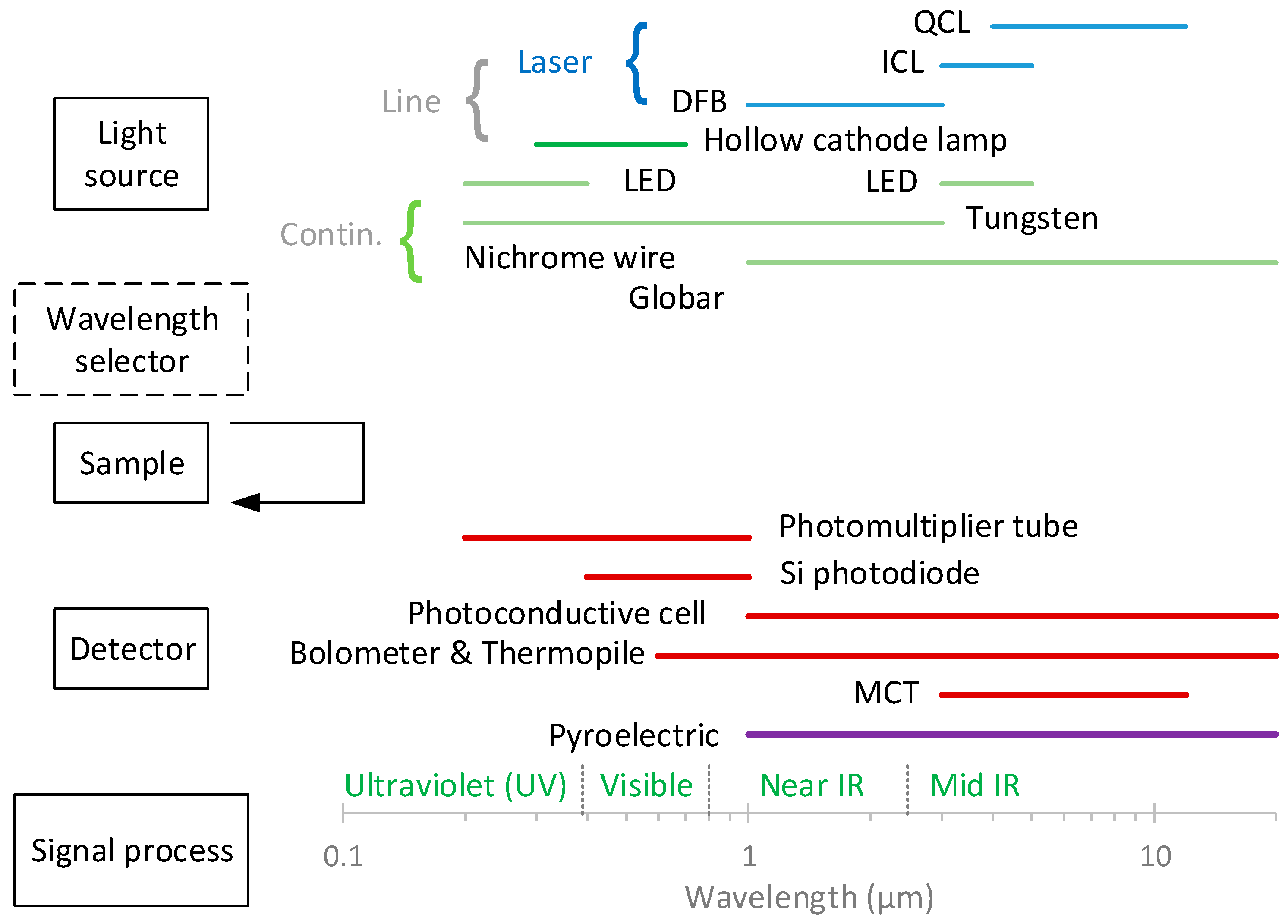
In absorption spectroscopy, the amount of light absorbed as a function of the wavelength is measured. Most spectroscopic instruments in the ultraviolet (UV), visible, and infrared (IR) regions are made up of five components [21,22,23,24,25,26] (Figure 1):
- (1)
- A stable source of radiant energy. The sources are classified as (i) continuum sources, which emit radiation that minorly changes in intensity as a function of the wavelength, such as light-emitting diodes (LEDs) and lamps, and (ii) line sources, which emit spectral lines in a very narrow wavelength range, for example, lasers. There are various types of lasers (e.g., gas, solid-state, and dye lasers), with semiconductor ones (diode and quantum cascade lasers) being commonly used in absorption spectroscopy [26];
- (2)
- A wavelength selector (optionally), such as a monochromator or a filter, which is used to isolate a limited region of the spectrum. Some instruments (dispersive spectrometers or spectrophotometers) use a spectrograph to spread out, or disperse, the wavelengths, so that they can be detected with a multichannel detector;
- (3)
- The sample region (cell);
- (4)
- A radiation detector, which is used to convert radiant energy to a measurable electrical signal. They are classified in (i) photon (or quantum) detectors, such as photomultiplier tubes [25], and (ii) heat transducers, e.g., pyroelectric detectors;
- (5)
- A signal-processing and readout unit.

Figure 1.
Main parts of spectroscopic instruments. Based on [21]. The arrow indicates that with IR radiation, the positions of the sample and wavelength selector are reversed. DFB = distributed feedback; ICL = interband cascade laser; IR = infrared; LED = light-emitting diode; MCT = mercury cadmium telluride; QCL = quantum cascade laser.
The components of infrared instruments differ from those of UV- and visible-range instruments. For example, IR sources are heated solids rather than deuterium or tungsten lamps, and infrared gratings are much coarser than those required for UV and visible radiation [21]. With IR radiation, the positions of the sample and wavelength selector are reversed (see Figure 1).
Fourier transform and filter photometer instruments are non-dispersive in the sense that they do not use a grating or prism to disperse radiation into its component wavelengths. An example of a filter photometer is a non-dispersive infrared (NDIR) sensor used to detect gases such as CO and CO2 [27,28,29]. The majority of NDIR sensors use broadband lamps or LED sources and an optical filter to select a narrow-band spectral region that overlaps with the absorption region of the gas of interest [30,31].
Fourier transform IR (FTIR) instruments contain no dispersing element, and all wavelengths are detected and measured simultaneously using a Michelson interferometer [32]. The interferogram is subsequently decoded by Fourier transformation. Detectors are typically pyroelectric transducers or photoconductive transducers, such as mercury cadmium telluride (MCT). FTIR instruments utilize lamps or LEDs as light sources. The application of FTIR spectrometers covers a very wide range: geology, chemistry, materials, medicine, and biology, using solid, liquid, and gaseous samples [33,34,35,36]. FTIR instruments have been extensively used to measure gaseous pollutants in many fields, e.g., ambient air [37], buildings [38], locomotives [39], thermal runaway and the release of gases from batteries [40], and exhaust gases [41,42] (see review in [32]).
Instruments that use lasers as light sources do not need wavelength selectors. Laser absorption spectroscopy (LAS) has been applied in many fields, such as breath analysis, atmospheric environment monitoring, industrial applications, and combustion diagnostics [26,43,44]. Tunable diode laser absorption spectroscopy (TDLAS) uses diode lasers that can be tuned in their emission wavelength by altering the temperature or the injection (drive) current of the laser itself. Diode lasers are operated at room temperature and offer bright, monochromatic light. Commonly used lasers are vertical-cavity surface-emitting lasers (VCSELs) and distributed feedback (DFB) laser diodes. Algorithms to minimize disturbances have been developed [45,46,47]. TDLAS has been applied in atmospheric monitoring [48,49,50,51,52], industrial monitoring [53], combustion exhaust [54,55,56,57,58,59] for various gases, and also for NH3 [60,61]. Other lasers commonly used in instruments are interband cascade lasers (ICLs) and quantum cascade lasers (QCLs) [62]. QCLs are unipolar coherent light sources emitting in the mid-infrared part of the electromagnetic spectrum. They represent an alternative to traditional diode lasers, which cannot emit light in the mid-infrared range. QCLs can be designed to emit in the wavelength region from below 4 μm to more than 10 μm. QCLs for N2O detection have been studied by many researchers [63,64,65,66,67,68,69,70], but ICLs have also been researched [71]. QCLs for engine exhaust measurements have also been employed for many years [72,73].
For regulatory vehicle emission measurements, “standard” laboratory-grade analyzers with well-defined principles of operation are prescribed: NDIR analyzers for CO and CO2, flame ionization detectors (FIDs) for hydrocarbons, and chemiluminescence analyzers (CLAs) or non-dispersive ultraviolet detectors (NDUVs) for NOX. For NH3 measurements, FTIR instruments, QCLs, or laser diode spectroscopy (LDS) can be used. FTIR spectrometry, which is a method used for NH3 detection, is not included in the regulations for the measurement of other gaseous components.
1.3. Objectives
Even though the measurement of “non-regulated” pollutants with FTIR and TDLAS instruments is common, there are not many studies that have assessed their accuracy. Furthermore, their accuracy in the measurement of “regulated” pollutants has not been established. To this end, in this study, we compare various instruments applying principles defined in the regulations with “non-standard” ones, focusing on light absorption instruments. Special emphasis is given to NH3, because it is a compound that is sensitive to the sampling conditions. With the exception of a few studies, most evaluation studies have been carried out with older-technology vehicles, or they are >10 years old; for some instruments (e.g., TDLAS), there are only a few studies on vehicle exhaust gas [74].
2. Materials and Methods
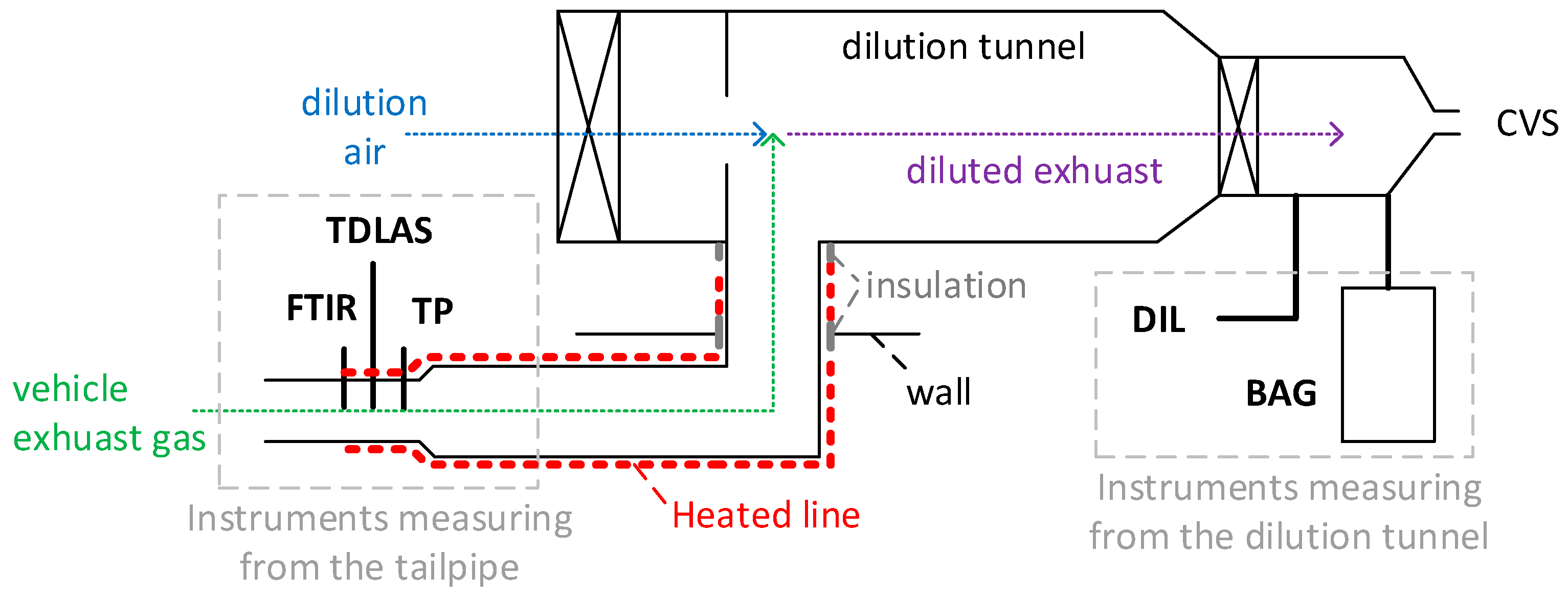
The tests were carried out by using the chassis dynamometer of the vehicle emissions laboratory (VELA 8) of the Joint Research Centre in Ispra, Italy. Figure 2 presents the setup, which was identical for all three vehicles tested. The vehicles, which were selected to cover a wide range of emission levels for all pollutants, included two Euro 6b gasoline direct injection vehicles (G1 and G2) and a Euro 6d-Temp diesel vehicle (D). Their technical specifications can be found in Table 1.
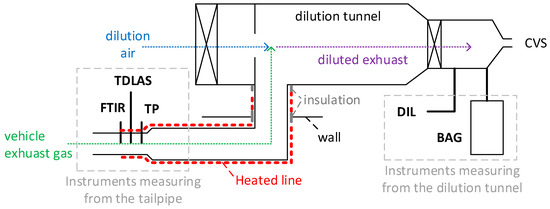
Figure 2.
Experimental setup. Thick continuous black lines are sampling lines. Dotted lines show the exhaust and air flow. Dashed lines are used for explanations. More details about the instruments in Table 2. CVS = constant-volume sampling; DIL = analyzer bench at the dilution tunnel; FTIR = Fourier transform infrared; TDLAS = tunable diode laser absorption spectroscopy instrument; TP = analyzer bench at the tailpipe.

Table 1.
Characteristics of test vehicles. The roadloads refer to F0 (N)/F1 (N/(km/h))/F2 (N/(km/h)2), as taken from the certificate of conformity (CoC) of the vehicles.
According to European light-duty vehicles exhaust regulation 2017/1151 [75], the exhaust emissions should be determined by collecting diluted exhaust gas in bags and analyzing them at the end of the test (see BAG in Figure 2). This method gives an integrated result per test (or a phase of a test), but no real-time information. For this reason, together with the fact that the bag results were available only for a limited number of tests, real-time measurements at the tailpipe and dilution tunnel were also carried out.
The vehicle exhaust gas was transferred to a dilution tunnel with constant-volume sampling (CVS) via a ~6 m line, where it was mixed with filtered air. The first 4.5 m of the transfer line was heated to 50 °C, and the last meter, to 75 °C. An additional 0.2 m section through the wall and a 0.2 m section connecting the transfer line to the tunnel were insulated. The total diluted flow rate was determined with critical Venturi orifices, which were calibrated annually. The range of the total flow rate was 7.5 to 10 m3/min depending on the vehicle and the test cycle. The dilution air flow rate was determined with an ultrasonic flow meter (Flowsonix; AVL, Austria, Graz). The exhaust flow rate was calculated as the difference between total diluted air flow rate and the dilution air flow rates.
Table 2 gives an overview of the instruments, the components they could measure, and their principles of operation. Table 2 also comments on which principle of measurement the EU light-duty regulation requires. Laboratory-grade analyzers were placed at the dilution tunnel (DIL) and the outlet of the vehicle tailpipe (TP) for measurement. The DIL bench was also used at the end of the measurements to analyze the diluted exhaust gas that was collected in bags (BAG) (available only for a few tests). The two benches included NDIR analyzers for CO and CO2, a chemiluminescence analyzer (CLA) for NOX (in regulations, NOX is defined as the sum of NO and NO2), a flame ionization detector (FID) with a non-methane cutter (NMC) for CH4, and a QCL-IR analyzer for N2O (only in the DIL bench). The CO and CO2 measurements were performed with dry exhaust (i.e., the exhaust sample was cooled down to remove the water content). A dry-to-wet correction [76] was applied based on the H2O concentration measurement (CH2O (%)) of the FTIR spectrometer (=1 − CH2O/100).
Table 2.
Analyzers used in this study. See Figure 2 for sampling points.
An FTIR spectrometer and a portable NH3 instrument, which will be described below, were also connected to the tailpipe. Great care was taken to also have some heating around the connection points between the instruments and the tailpipe, in order to minimize any condensation and NH3 losses. A heated blanket at 50 °C was used for this purpose.
The FTIR instrument (SESAM i60; AVL) comprised a spectrometer, a multi-path gas cell with a 2 m optical path with a working pressure of 860 hPa, a downstream sampling pump (6.5 L/min sampling rate), a Michelson interferometer (spectral resolution: 0.5 cm−1; spectral range: 650–4000 cm−1), and a liquid-nitrogen-cooled mercury cadmium telluride (MCT) detector; it had an acquisition frequency of 1 Hz. The instrument was connected to the tailpipe with a heated polytetrafluoroethylene (PTFE) sampling line at 191 °C including a heated pre-filter.
The portable NH3 detection instrument was an AVL mobile on-board vehicle evaluation (MOVE) module based on near-infrared TDLAS. It had a photo-based detector with high sensitivity and thus did not need a multi-path cell. The instrument was connected to the tailpipe with a sample line at 170 °C to limit any condensation of chemical byproducts (hang-up effects). The internal temperature of the sample path was kept constant at 170 °C, and the diode laser itself, at 60 °C, to avoid any shift in wavelength. Furthermore, water compensation was applied internally based on internal H2O measurement. The declared measurement accuracy was ±1.5 ppm or 1.5% of the reading (whichever was larger) for concentrations up to 1000 ppm, and 2% of the reading for concentrations of 1000–1500 ppm. TDLAS, a category of laser diode spectroscopy (LDS), fulfils the requirements of the current regulations, which prescribe FTIR, QCL, or LDS for the measurement of NH3 (see Table 2).
The technical details of the other instruments are not known. However, they fulfilled the linearity requirements of the regulation: slope of 0.99–1.01, R2 ≥ 0.998, SEE (standard error of estimate) ≤ 1% max, and offset ≤ 0.5% max. The accuracy was ±2% of the reading or ±0.3% of the full scale (whichever was larger). The t10–90 of all instruments was 2–2.5 s.
As a final note, light absorption spectrometry includes NDIR, FTIR, QCL, and TDLAS principles. CLA (NOX) and FID (CH4) results are presented for completeness. As it was mentioned, the bag results will not be provided, but the comparison of the DIL and bag results was excellent, with slopes of 1.00–1.05 and R2 > 0.99 (except for CH4: slope of 1.2 and R2 = 0.85).
The test cycles were selected in order to cover a wide range of driving conditions encountered in real life, cover a wide area of the engine map, and challenge the emission control devices over a wide range of boundary conditions. They included the following: (i) Type 1 approval cycles: new European driving cycle (NEDC) applicable until 2017 and the worldwide harmonized light-vehicle test cycle (WLTC) applicable since 2017; (ii) the Transport for London urban interpeak (TfL) cycle, representing urban driving with traffic; and (iii) the German Bundesautobahn (BAB) “federal highway” cycle, representing high-speed motorway driving up to 130 km/h with frequent and sharp accelerations from 80 to 130 km/h and from 110 to 130 km/h. Furthermore, some steady-speed driving was performed to investigate specific conditions or to regenerate the DPF of the diesel vehicle. For one test, the FTIR and TDLAS instruments (NH3 PEMSs) were swapped, and the test (BAB) was repeated. The relative difference between the two instruments remained the same, indicating that the impact of the two locations on the emissions was small, if any. All tests were performed at a 23 °C (±2 °C) ambient temperature, except the TfL test and a few BAB tests immediately after the TfL test, which were performed at 0 °C (±2 °C). The main statistics of the test cycles are summarized in Table 3.
Table 3.
Characteristics of test cycles. For cycles in which cold-start tests were carried out, the first 300 s and the rest of the cycle are given separately (separated with |).
For the calculations, the equations in UNECE Regulation 49 were followed for both raw (tailpipe) and diluted exhaust gas sampling. In short, the concentrations of the analyzers were multiplied by the exhaust gas flow or the dilution tunnel flow rate and corrected with a constant value depending on the compound; the fuel; and the sampling location (raw or diluted), which takes into account the density of the compound (see also [77]). Dry-to-wet correction was applied to analyzers measuring “dry” exhaust (NDIR analyzer for CO and CO2). No NOX humidity correction factor was applied, as it would have been the same for all NOX instruments (0.91 for tests at 23 °C and 0.75 for tests at 0 °C). Time alignment is not critical for dilution tunnel instruments, as the concentrations of the analyzers are multiplied by the constant flow rate of the dilution tunnel. However, it is important for instruments connected to the tailpipe. The FTIR CO2 signal was time-aligned with the exhaust flow; then, the other instruments’ signals were time-aligned with the respective compounds of the FTIR instrument, which had the same response due to its principle of operation. Appendix A describes a speed ramp test and explains in more detail the calculation methodology, as well as some correction factors.
3. Results and Discussion
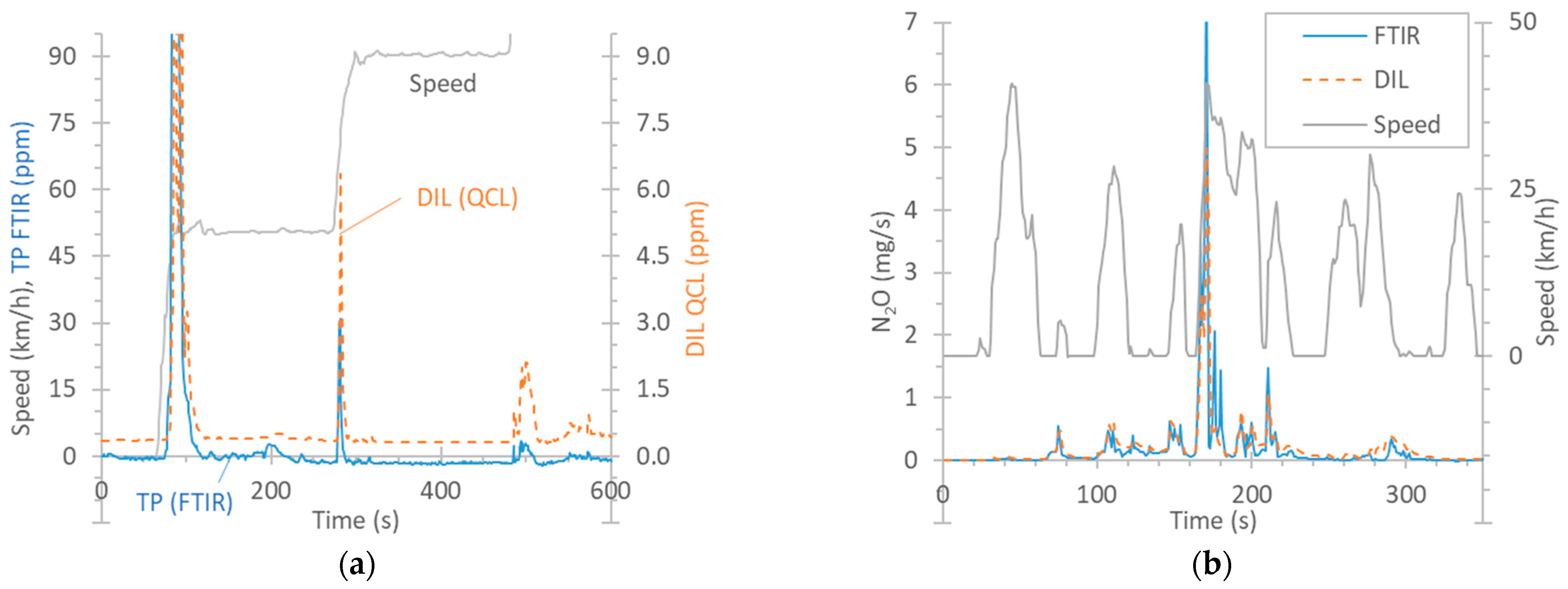
Figure 3a plots the real-time concentrations of N2O for a speed ramp test of vehicle G2 starting with a cold engine at 23 °C. N2O appeared during the first acceleration phase from an idle position to 50 km/h (note that the maximum of the peak is not shown in order to focus on the low concentrations). A smaller spike appeared in the second phase of acceleration to 90 km/h, and an even smaller one, in the phase of acceleration to 130 km/h. The signals of the two Instruments are not comparable, because one was connected to the dilution tunnel, and the other, to the tailpipe. Their difference includes the dilution factor in the dilution tunnel, which is variable, as it depends on the exhaust flow, especially during the transitions where N2O appeared.
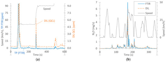
Figure 3.
Comparison of instruments measuring N2O: FTIR instrument at the tailpipe (TP) vs. QCL at the dilution tunnel (DIL). (a) Example of real-time concentrations (G2, speed ramp with cold start at 23 °C). (b) Real-time example (G2, cold-start TfL cycle at 0 °C).
The QCL at the dilution tunnel had a background level of around 0.35 ppm N2O originating from the dilution air of the tunnel. The FTIR instrument at the tailpipe, although it started at 0 ppm, after 200 s, it had an offset of −1 ppm. This value was up to −2 ppm in some tests. While the dilution tunnel background was taken into account in the calculations, the FTIR offset was not. The reason is that this offset was not observed at the beginning of the test but only after exhaust gas had been measured for some time. This has to do with the “interference” from other components of the exhaust gas when the cycle began and the engine was started. For N2O, the interfering gases can be CO, CO2, or H2O, depending on the wavelength [32]. This offset was also noticed in cycles that started with a warm engine, for which the condensation should be minimum, e.g., BAB tests. In hot cycles, at the beginning of the cycle, the zero level was around −0.4 ppm. Although still within the limit of quantification of the specific gas (0.4 ppm) [78], it indicates small temperature stabilization effects as the exhaust gas heats up the sampling lines and enters in the detection cell at a higher temperature.
Figure 3b presents an example of N2O emissions during the first 5 min of a cold-start TfL cycle at 0 °C, where the emission levels were very high (65 mg/km). The signals are now comparable because they are expressed in mg/s (they were multiplied by the dilution tunnel flow or the exhaust flow). The agreement among the instruments over the 5 min period (in mg/km) was satisfactory (10%) considering the uncertainty associated with the quantification of the exhaust flow rate and the data alignment required for the calculation of the emissions measured at the tailpipe.
N2O forms in the TWC, with the maximum occurring at around 200 °C [79,80,81], in the presence of NO, CO, and HC. Temperatures starting at 250 °C and higher do not produce any N2O [79], or the production is low [80]. Regarding diesel vehicles, N2O can form in DOCs, which are used to increase the NO2 fraction in the exhaust to promote the passive regeneration of the DPF or to improve deNOX activity in SCR [82]. N2O also forms during the rich regeneration of the lean NOX trap (LNT) catalyst. N2O can also form in SCR in excess of NH3 [83]. ASCs can also further contribute to the formation of N2O via the unselective oxidation of unreacted NH3 [82]. Vehicle D in our study (no LNT catalyst, but with a DOC, SCR, and an ASC) produced N2O during the whole WLTC, with cycle emissions of the order of 8 mg/km. A review study reported emission levels between 3 and 37 mg/km for diesel vehicles and between 0.1 and 14 mg/km for gasoline vehicles [78].
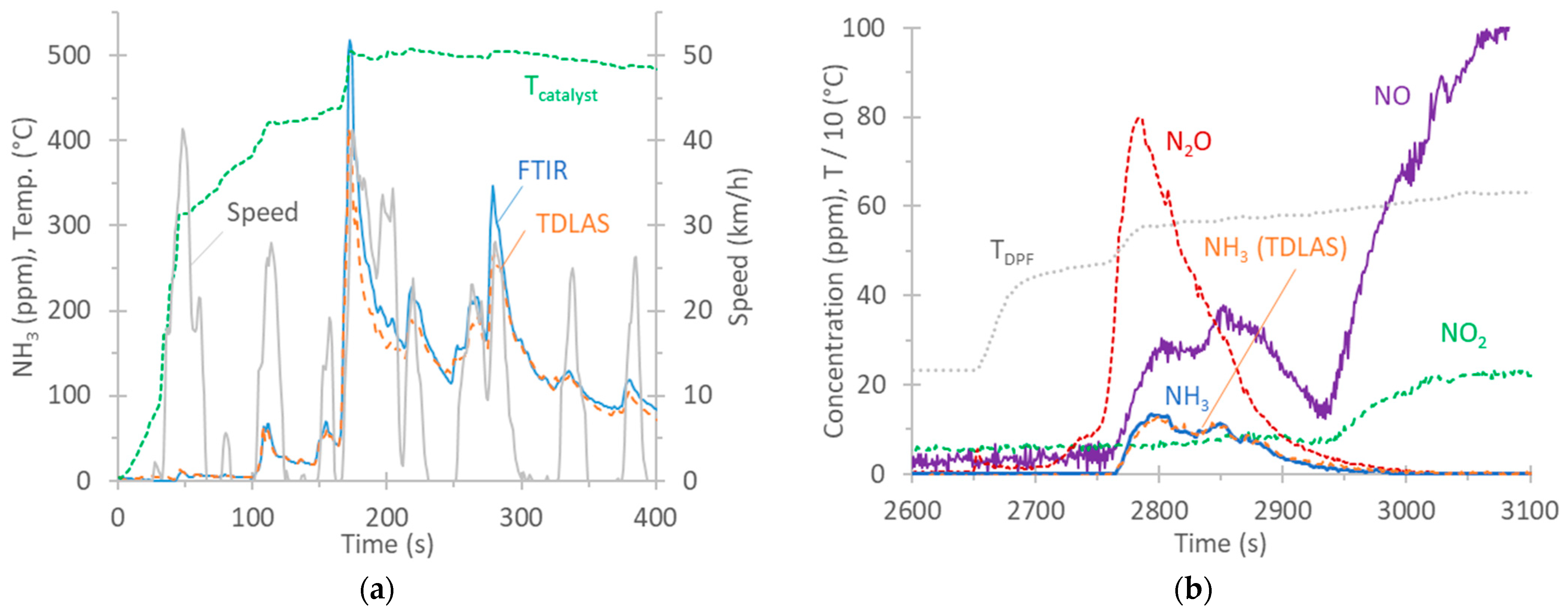
Figure 4a plots the real-time NH3 concentrations of vehicle G1 over the cold-start TfL cycle at a 0 °C ambient temperature. The catalyst’s temperature, as given by the vehicle from the on-board diagnostics (OBD) port, is also plotted. At the beginning of the cycle, there was no NH3. It appeared at approximately 100 s and reached the maximum levels at around 180 s. The agreement between the two instruments was good, with the FTIR analyzer recording 12% higher measurements than the TDLAS analyzer over this 5 min period.
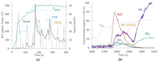
Figure 4.
Examples of real-time NH3 concentrations. FTIR and TDLAS analyzers are both at the tailpipe. (a) G1, cold-start TfL cycle at 0 °C; (b) D, 80 km/h regeneration at 23 °C. All measurements performed with FTIR analyzer, except the curve indicating NH3 (TDLAS analyzer).
According to the literature, NH3 forms within TWCs through reactions involving NO, CO, H2O, and H2 as precursor molecules [84,85], particularly under rich conditions [86]. A wide temperature range between 250 °C and 550 °C where NH3 selectivity was the highest has been reported [87]. NH3 formation is minimized in a temperature range 150 °C to 250 °C [79]. During acceleration phases, spikes appear due to a reduction in engine lambda promoting TWC selectivity towards NH3 [84,88,89,90].
All tests with vehicle D had zero NH3 emissions, except during a regeneration event. In the case of diesel vehicles, NH3, produced by the hydrolysis of urea solution, is used to reduce NOX to N2 and H2O in the SCR process. Ammonia slip catalysts (ASCs) are used to convert excess NH3 to N2 and H2O. Possible side reactions involve the unselective oxidation of NH3 to NO or N2O, among others [82]. Figure 4b plots the real-time concentrations of NO, NO2, NH3, and N2O over a regeneration event at 80 km/h for vehicle D. The NH3 concentrations measured with the TDLAS analyzer (NH3 PEMS) are also plotted and were in very good agreement with those of the FTIR analyzer (max concentration of 14 ppm). The regeneration started at approximately 2650 s, as the sharp increase in the temperature at the DPF indicates. The increase in pollutants started at 2750 s, while at 2950 s, only NO and NO2 remained. The high N2O concentration is likely due to unselective ammonia oxidation (at temperatures >400 °C and low NO2) [91,92,93]. Then, NH3 decreased, while NO and NO2 further increased. It is likely that urea injection was minimized or stopped at 2950 s, as the NOX conversion efficiency at such high temperatures is low due to thermodynamic limitations [94,95].
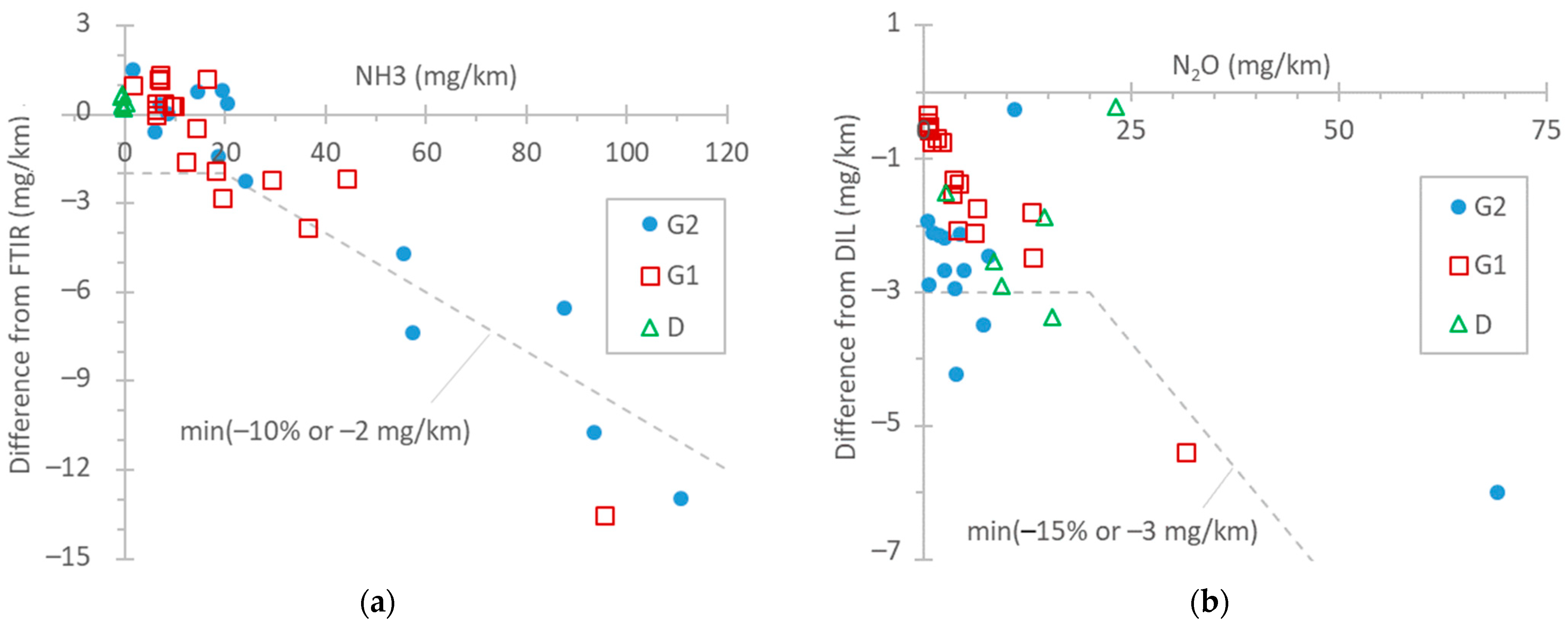
Figure 5a summarizes the NH3 differences between FTIR and TDLAS instruments, with both being connected to the tailpipe. For concentration levels up to 20 mg/km (the proposed Euro 7 limit for light-duty vehicles), the differences were within 2 mg/km for the test cycles WLTC and NEDC. Such differences between FTIR and QCL instruments have also been reported by other studies [96,97]. At higher emission levels (TfL tests at 0 °C and particularly BAB tests), the TDLAS analyzer recorded approximately 10% lower values. The FTIR analyzer was checked before the measurement campaign with a 520 ppm NH3 gas cylinder (both bypassing and measuring with the sampling line) and recorded 2% higher values. The instrument manufacturer checked the TDLAS analyzer after the measurement campaign, and the concentration was <1% lower than the reference concentration of the cylinder (around 580 ppm). Thus, the difference could not have been due to the calibration of the NH3 detectors. For NH3, the humidity in the exhaust gas plays an important role, as it condensates on the tubing, sampling probes, and sampling lines of the instruments, where NH3 can be adsorbed and later released (see Appendix A, Figure A2). The 10% difference is acceptable and in agreement with the literature [32,69]. Even though the calibration of the instruments can be much more accurate, the dynamic phenomena described previously play an important role.
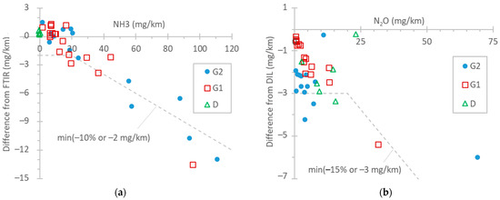
Figure 5.
Comparison of instruments measuring NH3 and N2O: (a) NH3: TDLAS vs. FTIR both at the tailpipe; (b) N2O: FTIR at the tailpipe vs. QCL at the dilution tunnel (DIL). Dotted lines are only meant to aid the eye.
In the literature, the ammonia levels of gasoline light-duty vehicles span over a wide range, with average values of around 30–70 mg/km [98,99], but modern vehicles have, in general, lower emissions [89,98,99,100,101,102,103]. However, since NH3 emissions from TWC-equipped vehicles can increase with mileage [104,105], it is not clear whether this has to do with the lower mileage of the vehicles or different engine operation aftertreatment strategies. Vehicle D in our study, equipped with an ASC, had negligible NH3 emissions, in agreement with other studies [106]. However, non-zero emissions from diesel light-duty vehicles have been reported [100,107].
Figure 5b gives an overview of the differences between the FTIR analyzer at the tailpipe and the QCL at the dilution tunnel (DIL) for N2O emissions. In general, the differences were <15% or within 3 mg/km. However, the main reason for these 2–3 mg/km differences is the 1–2 ppm offset (due to interferences) of the FTIR analyzer. It should be recalled that the N2O background (around 0.35 ppm, constant) was corrected for the instrument connected to the dilution tunnel. This correction, for the dilution tunnel flow rates (7.5–10 m3/min), was equivalent to 2–7 mg/km for the NEDC, WLTC, and BAB tests and to 11–24 for the TfL test and the cold-start part (5 min) of the NEDC and WLTC. Other studies have found even smaller differences (±1 mg/km) [97]. To put the results into perspective, the N2O limit of China 6 passenger cars is 20 mg/km. On-road and laboratory measurements have reported values in the 10–20 mg/km range for diesel vehicles [78,108,109].
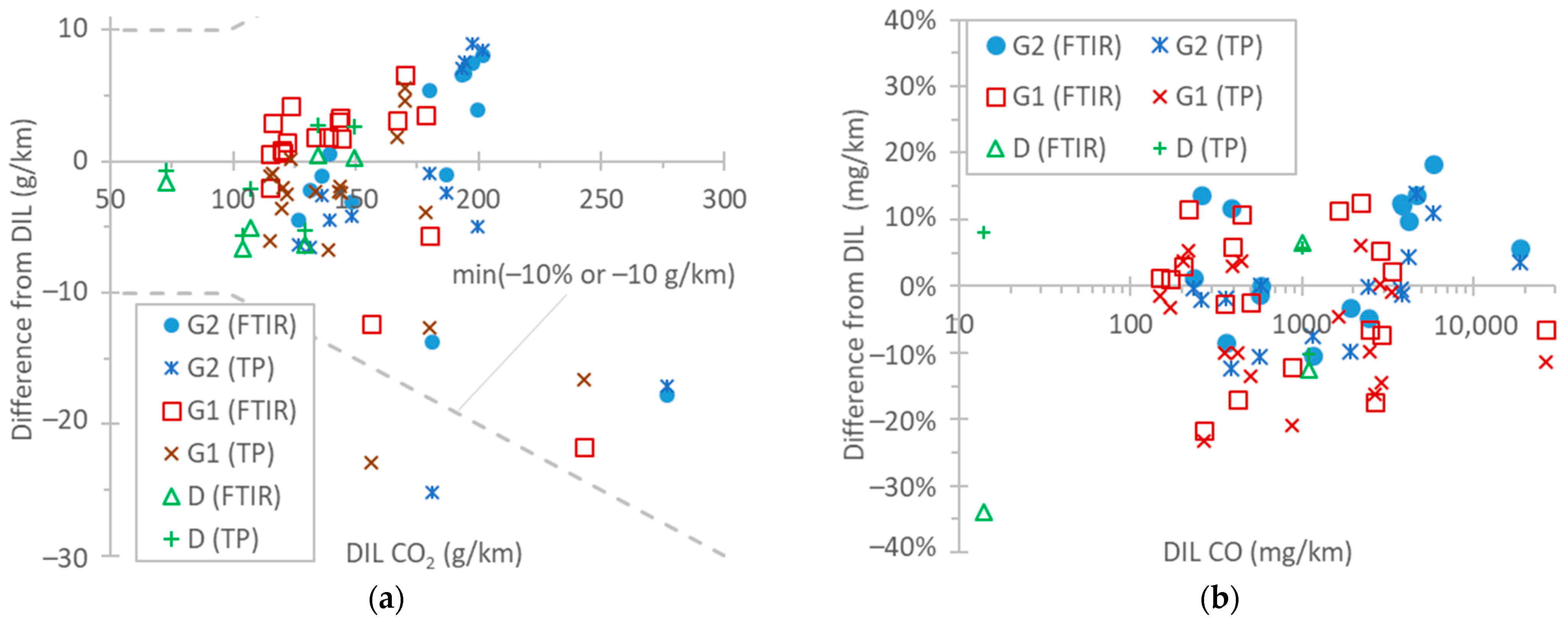
Figure 6a plots the CO2 differences among the instruments. It should be recalled that the FTIR analyzer was used to measure “wet” exhaust, and the NDIR analyzer, “dry” exhaust, applying a dry-to-wet correction to convert this to the “wet” value (see Materials and Methods). This correction was around 0.85 for the gasoline vehicles, and 0.90 for the first 300 s of the cold-start tests. For the dilution tunnel, the diluted exhaust dry-to-wet correction for the NDIR analyzer was very small (<2%). In general, the CO2 differences between the NDIR instruments at the two locations were well within ±10 g/km or ±10%. The few exceptions with higher differences were found in the TfL cycle at 0 °C. The high condensation resulted in higher uncertainty in the dry-to-wet correction. Furthermore, the exhaust flow rate determined with air flows had higher uncertainty, as a comparison with the CO2 method showed higher differences in the low range (see Appendix A). A closer look at the data reveals that the two instruments at the tailpipe (FTIR and NDIR instruments) were within 5 g/km or 5%, further supporting that the remaining 5% differences from the dilution tunnel instrument were mainly due to uncertainties in the exhaust flow determination. Nevertheless, 5–10% differences in CO2 measurements are acceptable and of the same order of values in other studies with similar technologies [32,69,77,97,109,110,111,112,113].
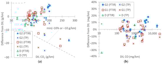
Figure 6.
Comparison of instruments. Reference NDIR instrument at the dilution tunnel (DIL) vs. FTIR instrument at tailpipe and NDIR instrument at the tailpipe (TP): (a) CO2; (b) CO. Dotted lines are only meant to aid the eye.
Figure 6b plots the differences in CO instruments over a wide range of emission levels: from a few mg/km up to 30,000 mg/km. The highest levels were measured during the first 5 min of the cold-start cycles, in particular the TfL test at 0 °C. Both instruments at the tailpipe (FTIR “wet” and NDIR “dry” instruments) were within ±20% from the instrument at the dilution tunnel (NDIR) for the whole concentration range. The FTIR instrument differed from the NDIR instrument at the tailpipe by −10% to 20%. To put the results into perspective, the Euro 6 limits are 500 mg/km for diesel vehicles and 1000 mg/km for gasoline vehicles. Another study found 15% or 50 mg/km differences between a QCL and an NDIR instrument [97] for emissions up to 1085 mg/km, while PEMSs (NDIR instruments) typically show 15% differences [111] or less [114] from laboratory NDIR equipment.
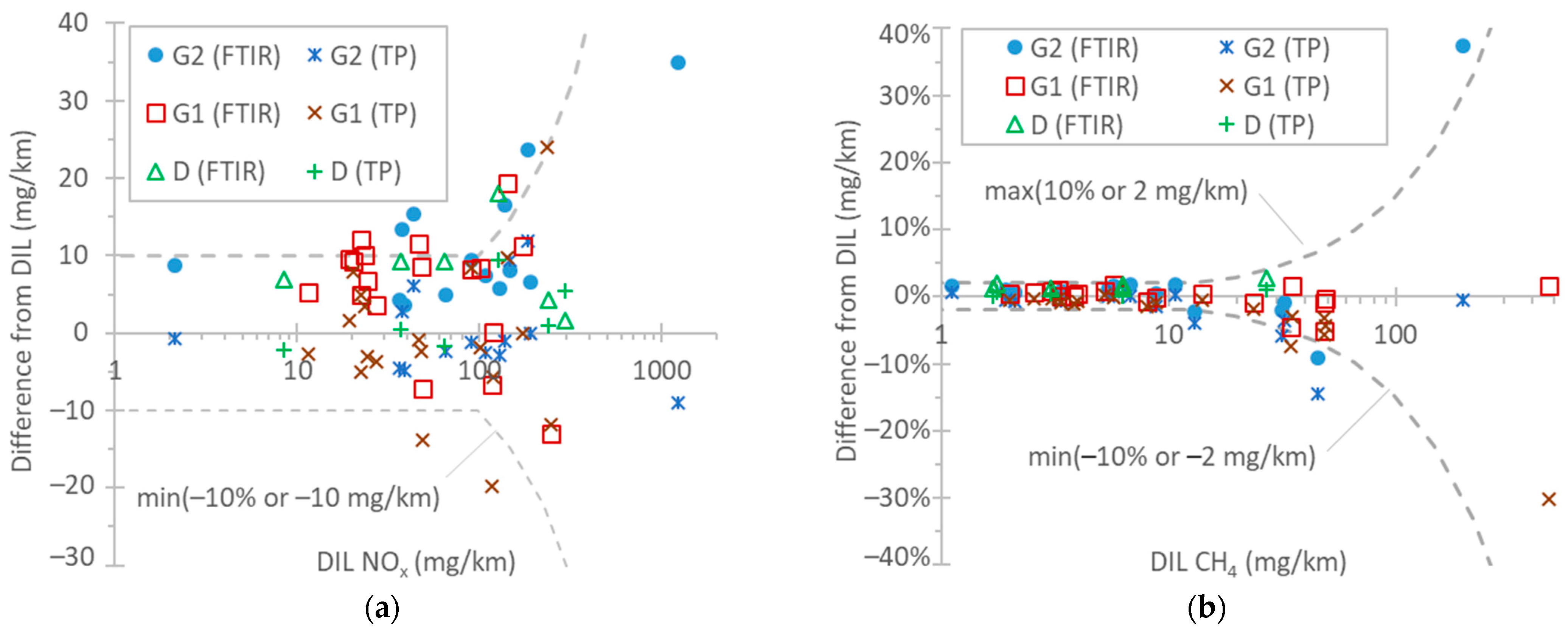
Figure 7a plots the NOX differences among the instruments. The emission levels were from a few mg/km up to 1250 mg/km. With a few exceptions, the difference between the CLA at the tailpipe and the CLA at the dilution tunnel was within 10 g/km or 10%. The two exceptions were the TfL tests at 0 °C. The FTIR analyzer showed similar differences, reaching 15 mg/km in a few cases. Comparing the FTIR analyzer with the CLA at the tailpipe, the former recorded, on average, 8 mg/km higher values. CLAs have some uncertainties due to the use of NO2-to-NO converters with conversion efficiencies >95% (which need to be checked every month according to EU regulation), possible NO2 losses in their chiller, and influence exerted by quenching with water and CO2 [115]. FTIR instruments’ NO2 measurement is affected by water vapor interference. Differences of 5–15% have also been reported for instruments measuring light-duty vehicle and heavy-duty engine exhaust gas [69,77,111,112,113]. Studies with light-duty vehicles found differences in instruments of around 10 mg/km for up to 80 mg/km emission levels [97,116] and a 5 mg/km difference for levels of around 15–45 mg/km [114,116]. However, higher differences of the order of 20% [109] or higher [110,113] have also been reported in the past.
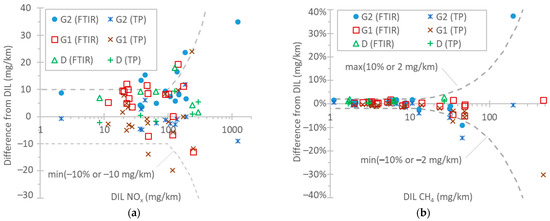
Figure 7.
Comparison of instruments measuring the following: (a) NOX: reference CLA at the dilution tunnel (DIL) vs. FTIR instrument at the tailpipe and CLA at the tailpipe (TP); (b) CH4: reference FID with non-methane cutter at the dilution tunnel (DIL) vs. FTIR instrument at the tailpipe and FID with non-methane cutter at the tailpipe (TP). Dotted lines are only meant to aid the eye.
Figure 7b plots the CH4 differences among the instruments. The emission levels ranged from a few mg/km up to 500 mg/km. The differences between the FTIR instrument/the FID with a non-methane cutter at the tailpipe and the FID with a non-methane cutter at the dilution tunnel were within 2 g/km or 10%. The highest differences exceeding 10% were found in the cold-start TfL test at 0 °C and the WLTC. A previous study found a slope of 0.96 (R2 = 0.99) between FTIR measurements and CH4 from bags in the range 0–40 mg/km [109]. A recent study found 1–2 mg/km at levels up to 20 mg/km [97].
4. Conclusions
In this study, we compared instruments sampling at the tailpipe and the dilution tunnel. The benches at the dilution tunnel and at the tailpipe consisted of “standard” analyzers following the principles of operation described in the respective regulation: a non-dispersive infrared (NDIR) instrument for CO and CO2, a flame ionization detector (FID) with a non-methane cutter for CH4, and chemiluminescence analyzer (CLA) for NOX. Furthermore, the bench at the dilution tunnel included laser absorption with a quantum cascade laser (QCL) analyzer for N2O. A Fourier transform infrared (FTIR) spectrometer was also connected at the tailpipe for measuring all components. Finally, a portable instrument based on tunable diode laser absorption spectroscopy (TDLAS) for NH3 was connected to the tailpipe. One diesel and two gasoline vehicles running in different test cycles at ambient temperatures of 23 °C and 0 °C provided a wide range of emission levels. For the regulated pollutants, the differences between FTIR and “standard” analyzers were better than 10% for CO2, 20% for CO, and 10% for NOX and CH4. For CO and CO2, the wet or dry measurement with subsequent correction plays a role in the differences, especially in cold-start cycles. For NOX, water interference can impact the FTIR measurements. In all cases, the exhaust flow rate measurement accuracy had an impact on the results. For N2O, the difference between the FTIR and QCL analyzers was 3 mg/km or 15% (whichever was larger) due to the 1–2 ppm “offset” of the FTIR analyzer caused by the interference from other gases. Calibration of the FTIR instrument with “wet” (i.e., humidified) calibration gas by the instrument manufacturer is recommended. Wrong correction of the N2O background in the dilution air can also lead to significant errors in the N2O emissions from the dilution tunnel. The differences between FTIR and TDLAS instruments for NH3 were 2 mg/km or 10% (whichever was larger). This was mainly attributed to the adsorption and release of NH3 from the tubing, sampling probes, and sampling lines of the instruments. The results of this study support the use of “non-standard” techniques for the measurement of regulated (and non-regulated) pollutants without significant increases in measurement uncertainty over a wide range of emission levels. Special attention must be paid to NH3 measurement.
Author Contributions
Conceptualization, B.G. and R.S.-B.; methodology, A.M. and B.G.; formal analysis, B.G.; writing—original draft preparation, B.G.; writing—review and editing, A.M., J.F., M.C., R.S.-B. and V.V. All authors have read and agreed to the published version of the manuscript.
Funding
This research received no external funding.
Institutional Review Board Statement
Not applicable.
Informed Consent Statement
Not applicable.
Data Availability Statement
Data are available upon request from the corresponding author.
Acknowledgments
The authors would like to acknowledge the technical staff of VELA 8 (M. Centurelli and M. Stefanini) and AVL’s residence engineers (A. Bonamin and D. Zanardini) for running the tests. AVL (K. Oberguggenberger and R. Garda) is acknowledged for having provided the prototype instrument for the measurement of NH3.
Conflicts of Interest
Author Victor Valverde was employed by the company Unisystem S.A. The remaining authors declare that this research was conducted in the absence of any commercial or financial relationships that could be construed as potential conflicts of interest.
Disclaimer
The information and views set out are those of the authors and do not necessarily reflect the official opinion of the European Commission. Neither the European Union institutions and bodies nor any person acting on their behalf may be held responsible for the use which may be made of the information contained therein. Mention of trade or commercial products does not constitute endorsement or recommendation by the authors or the European Commission.
Appendix A
This appendix gives details for a speed ramp test, as an example, in order to better clarify some concepts mentioned in the main text. The vehicle drove at 50 km/h, 90 km/h, 130 km/h, and then back to 90 km/h and 50 km/h (Figure A1b). Figure A1a plots the CO2 concentration as measured by the FTIR instrument at the tailpipe (TP), the NDIR instrument at the tailpipe, and the NDIR instrument at the dilution tunnel (DIL). The H2O concentration, as measured by the FTIR instrument at the tailpipe, is also plotted. The CO2 difference between FTIR (“wet” measurement, i.e., with H2O) and NDIR (“dry” measurement, i.e., after removal of H2O) instruments at the tailpipe is evident for most of the cycle. Only at the beginning of the test, the two concentrations are close to each other due to condensation taking place on the vehicle’s exhaust tubing and aftertreatment devices; thus, exhaust gas with low H2O content arrives at both instruments. The “dry” measurements of the NDIR instrument can be converted to “wet” measurements by applying a dry-to-wet factor. This factor, according to Regulation (EU) 2017/1151 [75] is calculated based on the CO2, CO, and HC concentrations. The equation in the regulation assumes that no condensation or evaporation takes place. kCO2,CO,HC is plotted in Figure A1b. The same plot also gives the correction based on the H2O measurement of the FTIR instrument. The two curves are quite close for most of the cycle, except at the beginning, when condensation takes place. Note also that some evaporation takes place (around 300 s) before the two curves reach a constant small difference. The under-correction at the beginning of the cycle can result in differences when short cycles with cold start are compared. Detailed discussion on the topic can be found elsewhere [76].
For the instruments at the tailpipe, the exhaust flow rate is needed to convert the concentration (in ppm) to mass (in mg). The exhaust flow is calculated as the difference between the total diluted flow and the dilution air flow in the dilution tunnel (see Materials and Methods in the main text). Another possibility is to divide the total diluted flow rate with the dilution factor. The dilution factor can be calculated by using the ratio of CO2 concentration at the tailpipe and at the dilution tunnel corrected with the CO2 background of the dilution air. The exhaust flow rates calculated with the two methods are plotted in Figure A1b. The difference between the two exhaust flow rates is 18% in an idle position and at a speed of 50 km/h, but it is 1% at high speeds (130 km/h) resulting in a 6% difference for the whole speed ramp test (the -flows difference method results in lower values). The difference between the two flows at the same speed is similar in the ramp-up and -down phases (1% at 50 km/h and 5% at 90 km/h).
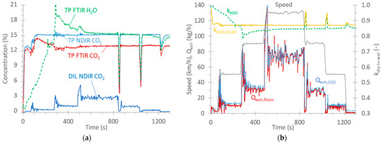
Figure A1.
Steady-speed ramp test with vehicle G2: (a) CO2 and H2O concentrations; (b) Speed profile, calculated exhaust flow rates based on flows at the dilution tunnel and dilution tunnel (Qexh,flows) or CO2 measurements at the tailpipe and dilution tunnel (Qexh,CO2). The dry-to-wet correction based on CO2, CO and HC (kCO2,CO,HC) measurements or H2O measurements is also plotted (kH2O).
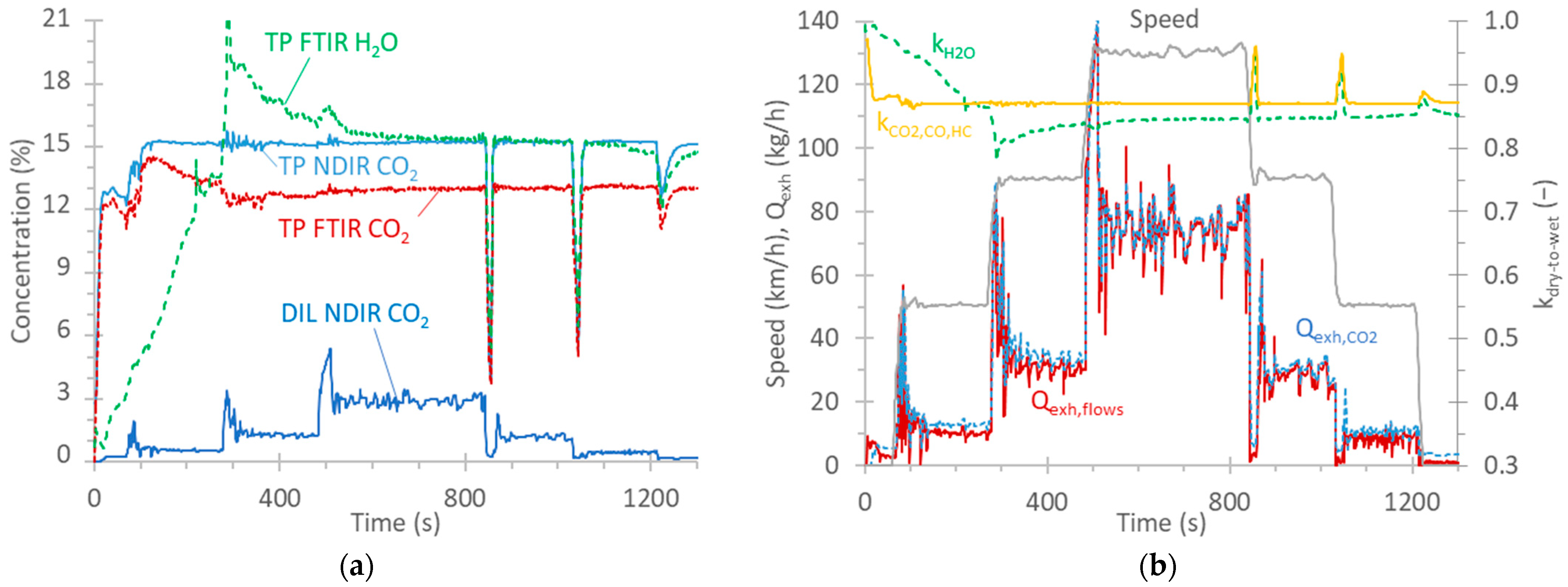
Figure A2a plots the NH3 emissions of the speed ramp tests with the FTIR and the TDLAS instruments (NH3 PEMSs), both connected to the tailpipe. In general, there is good agreement between the two instruments at the beginning of the test, with the FTIR instrument measuring higher values as the speed and concentration increase; then, at 130 km/h, the concentration drops, but the FTIR measurements are lower than the TDLAS ones. Note also some small spikes at 850 s and 950 s recorded by the TDLAS instrument (or lack of response of the FTIR instrument). At the end of the test, at the low speed of 50 km/h, as the concentration further increases, the two instruments get closer to each other, and at the end of the test, the FTIR instrument exceeds the TDLAS instrument.
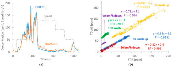
Figure A2.
Steady-speed ramp test with vehicle G2: (a) Speed profile and NH3 concentration. (b) Correlation of the two NH3 instruments at the tailpipe (FTIR and TDLAS instruments). Note that the 90 km/h and 130 km/h points are shifted upwards by 30 ppm and 60 ppm, respectively, for better visualization.

Figure A2b plots the correlation between the two instruments at various speeds (the transition points are not included). At 50 km/h, the slope is around 0.83 both when ramping up or down. The slope of the 90 km/h ramp-up from 50 km/h is also similar (0.84), while that of the ramp-down is lower (0.78), but the concentrations are low (<15 ppm). The 130 km/h phase has a slope of 1.2, indicating some desorption of stored NH3 for the TDLAS instrument or adsorption for the FTIR instrument.
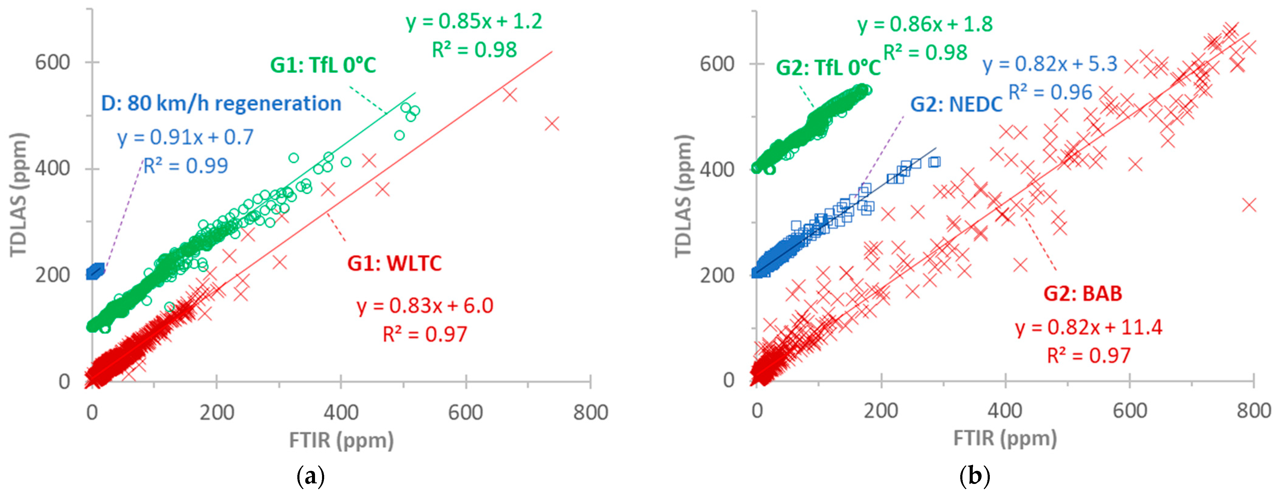
More correlations with more cycles for G2 (Figure A3b) and the other vehicles, D and G1 (Figure A3a), confirm the previous discussion. The highest scatter is observed in the dynamic BAB cycles. There is no indication of non-linearity at high concentrations. The slopes are around 0.85, and R2 > 0.96. For all vehicles and cycles, the slopes are 0.73–0.93 (0.85 to 0.95 when forcing through zero), and R2 > 0.9, with lower values for the dynamic BAB cycles. Even lower values are calculated for the BAB cycles at 0 °C (slope of 0.65 or 0.7 when forcing through zero). This indicates an ambient temperature impact on NH3 adsorption and release from the tubing, sampling probes, and sampling lines of the instruments.
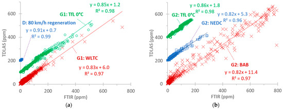
Figure A3.
Correlation of TDLAS and FTIR instruments for measuring NH3 at the tailpipe for various test cycles: (a) vehicles D and G1; (b) vehicle G2. Note that some cycles are shifted upwards for better visualization.
Figure A3.
Correlation of TDLAS and FTIR instruments for measuring NH3 at the tailpipe for various test cycles: (a) vehicles D and G1; (b) vehicle G2. Note that some cycles are shifted upwards for better visualization.
References
- United Nations. Climate Change The Paris Greement. 2023. Available online: https://unfccc.int/process-and-meetings/the-paris-agreement (accessed on 20 February 2024).
- Zubair, M.; Chen, S.; Ma, Y.; Hu, X. A Systematic Review on Carbon Dioxide (CO2) Emission Measurement Methods under PRISMA Guidelines: Transportation Sustainability and Development Programs. Sustainability 2023, 15, 4817. [Google Scholar] [CrossRef]
- United States Environmental Protection Agency (EPA) Sources of Greenhouse Gas Emissions. 2023. Available online: https://www.epa.gov/ghgemissions/sources-greenhouse-gas-emissions (accessed on 20 February 2024).
- Statista Transportation Emissions in the European Union—Statistics & Facts. 2024. Available online: https://www.statista.com/topics/7968/transportation-emissions-in-the-eu/#editorspicks (accessed on 20 February 2024).
- Intergovernmental Panel on Climate Change. Climate Change 2021—The Physical Science Basis: Working Group I Contribution to the Sixth Assessment Report of the Intergovernmental Panel on Climate Change, 1st ed.; Cambridge University Press: Cambridge, UK, 2021; ISBN 978-1-00-915789-6. [Google Scholar]
- Nisbet, E.G.; Manning, M.R.; Dlugokencky, E.J.; Fisher, R.E.; Lowry, D.; Michel, S.E.; Myhre, C.L.; Platt, S.M.; Allen, G.; Bousquet, P.; et al. Very Strong Atmospheric Methane Growth in the 4 Years 2014–2017: Implications for the Paris Agreement. Glob. Biogeochem. Cycles 2019, 33, 318–342. [Google Scholar] [CrossRef]
- Tian, H.; Xu, R.; Canadell, J.G.; Thompson, R.L.; Winiwarter, W.; Suntharalingam, P.; Davidson, E.A.; Ciais, P.; Jackson, R.B.; Janssens-Maenhout, G.; et al. A Comprehensive Quantification of Global Nitrous Oxide Sources and Sinks. Nature 2020, 586, 248–256. [Google Scholar] [CrossRef] [PubMed]
- Stell, A.C.; Bertolacci, M.; Zammit-Mangion, A.; Rigby, M.; Fraser, P.J.; Harth, C.M.; Krummel, P.B.; Lan, X.; Manizza, M.; Mühle, J.; et al. Modelling the Growth of Atmospheric Nitrous Oxide Using a Global Hierarchical Inversion. Atmos. Chem. Phys. 2022, 22, 12945–12960. [Google Scholar] [CrossRef]
- European Environmental Agency (EEA) Air Pollution in Europe: 2023 Reporting Status under the National Emission Reduction Commitments Directive. 2023. Available online: https://www.eea.europa.eu/publications/national-emission-reduction-commitments-directive-2023 (accessed on 20 February 2020).
- European Environmental Agency (EEA) Sources and Emissions of Air Pollutants in Europe 2022. Available online: https://www.eea.europa.eu/publications/air-quality-in-europe-2022/sources-and-emissions-of-air (accessed on 20 February 2020).
- Farren, N.J.; Davison, J.; Rose, R.A.; Wagner, R.L.; Carslaw, D.C. Underestimated Ammonia Emissions from Road Vehicles. Environ. Sci. Technol. 2020, 54, 15689–15697. [Google Scholar] [CrossRef]
- Chatain, M.; Chretien, E.; Crunaire, S.; Jantzem, E. Road Traffic and Its Influence on Urban Ammonia Concentrations (France). Atmosphere 2022, 13, 1032. [Google Scholar] [CrossRef]
- Walters, W.W.; Karod, M.; Willcocks, E.; Baek, B.H.; Blum, D.E.; Hastings, M.G. Quantifying the Importance of Vehicle Ammonia Emissions in an Urban Area of Northeastern USA Utilizing Nitrogen Isotopes. Atmos. Chem. Phys. 2022, 22, 13431–13448. [Google Scholar] [CrossRef]
- Wen, Y.; Zhang, S.; Wu, Y.; Hao, J. Vehicular Ammonia Emissions: An Underappreciated Emission Source in Densely Populated Areas. Atmos. Chem. Phys. 2023, 23, 3819–3828. [Google Scholar] [CrossRef]
- European Environmental Agency (EEA) National Emission Reduction Commitments (NEC) Directive. 2023. Available online: https://www.eea.europa.eu/en/topics/in-depth/air-pollution/necd (accessed on 20 February 2024).
- UNECE. The 1999 Gothenburg Protocol to Abate Acidification, Eutrophication and Ground-Level Ozone (Gothenburg Protocol). 1999. Available online: https://unece.org/environment-policy/air/protocol-abate-acidification-eutrophication-and-ground-level-ozone (accessed on 20 February 2024).
- DieselNet Emission Standards 2022. Available online: https://dieselnet.com/standards/ (accessed on 20 February 2024).
- Giechaskiel, B.; Joshi, A.; Ntziachristos, L.; Dilara, P. European Regulatory Framework and Particulate Matter Emissions of Gasoline Light-Duty Vehicles: A Review. Catalysts 2019, 9, 586. [Google Scholar] [CrossRef]
- United Nations Regulation 154: Worldwide Harmonized Light Vehicles Test Procedure (WLTP). 2021. Available online: https://unece.org/transport/vehicle-regulations-wp29/standards/addenda-1958-agreement-regulations-141-160 (accessed on 20 February 2024).
- Ribeiro, C.B.; Rodella, F.H.C.; Hoinaski, L. Regulating Light-Duty Vehicle Emissions: An Overview of US, EU, China and Brazil Programs and Its Effect on Air Quality. Clean Technol. Environ. Policy 2022, 24, 851–862. [Google Scholar] [CrossRef]
- Skoog, D.A.; Holler, F.J.; Crouch, S.R. Principles of Instrumental Analysis, 7th ed.; Cengage Learning: Boston, MA, USA, 2018; ISBN 978-1-305-57721-3. [Google Scholar]
- Hodgkinson, J.; Tatam, R.P. Optical Gas Sensing: A Review. Meas. Sci. Technol. 2013, 24, 012004. [Google Scholar] [CrossRef]
- Goldenstein, C.S.; Spearrin, R.M.; Jeffries, J.B.; Hanson, R.K. Infrared Laser-Absorption Sensing for Combustion Gases. Prog. Energy Combust. Sci. 2017, 60, 132–176. [Google Scholar] [CrossRef]
- Du, Z.; Zhang, S.; Li, J.; Gao, N.; Tong, K. Mid-Infrared Tunable Laser-Based Broadband Fingerprint Absorption Spectroscopy for Trace Gas Sensing: A Review. Appl. Sci. 2019, 9, 338. [Google Scholar] [CrossRef]
- Khan, S.; Newport, D.; Le Calvé, S. Gas Detection Using Portable Deep-UV Absorption Spectrophotometry: A Review. Sensors 2019, 19, 5210. [Google Scholar] [CrossRef] [PubMed]
- Fu, B.; Zhang, C.; Lyu, W.; Sun, J.; Shang, C.; Cheng, Y.; Xu, L. Recent Progress on Laser Absorption Spectroscopy for Determination of Gaseous Chemical Species. Appl. Spectrosc. Rev. 2022, 57, 112–152. [Google Scholar] [CrossRef]
- Zellweger, C.; Hüglin, C.; Klausen, J.; Steinbacher, M.; Vollmer, M.; Buchmann, B. Inter-Comparison of Four Different Carbon Monoxide Measurement Techniques and Evaluation of the Long-Term Carbon Monoxide Time Series of Jungfraujoch. Atmos. Chem. Phys. 2009, 9, 3491–3503. [Google Scholar] [CrossRef]
- Zhou, L.; He, Y.; Zhang, Q.; Zhang, L. Carbon Dioxide Sensor Module Based on NDIR Technology. Micromachines 2021, 12, 845. [Google Scholar] [CrossRef]
- Xu, M.; Peng, B.; Zhu, X.; Guo, Y. Multi-Gas Detection System Based on Non-Dispersive Infrared (NDIR) Spectral Technology. Sensors 2022, 22, 836. [Google Scholar] [CrossRef]
- Adachi, M.; Nakamura, H. Engine Emissions Measurement Handbook: HORIBA Automotive Test Systems; SAE International: Warrendale, PA, USA, 2014; ISBN 978-0-7680-8012-4. [Google Scholar]
- Dinh, T.-V.; Choi, I.-Y.; Son, Y.-S.; Kim, J.-C. A Review on Non-Dispersive Infrared Gas Sensors: Improvement of Sensor Detection Limit and Interference Correction. Sens. Actuators B Chem. 2016, 231, 529–538. [Google Scholar] [CrossRef]
- Giechaskiel, B.; Clairotte, M. Fourier Transform Infrared (FTIR) Spectroscopy for Measurements of Vehicle Exhaust Emissions: A Review. Appl. Sci. 2021, 11, 7416. [Google Scholar] [CrossRef]
- Guerrero-Pérez, M.O.; Patience, G.S. Experimental Methods in Chemical Engineering: Fourier Transform Infrared Spectroscopy—FTIR. Can. J. Chem. Eng. 2020, 98, 25–33. [Google Scholar] [CrossRef]
- Rohman, A.; Ghazali, M.A.B.; Windarsih, A.; Irnawati, I.; Riyanto, S.; Yusof, F.M.; Mustafa, S. Comprehensive Review on Application of FTIR Spectroscopy Coupled with Chemometrics for Authentication Analysis of Fats and Oils in the Food Products. Molecules 2020, 25, 5485. [Google Scholar] [CrossRef]
- Fadlelmoula, A.; Pinho, D.; Carvalho, V.H.; Catarino, S.O.; Minas, G. Fourier Transform Infrared (FTIR) Spectroscopy to Analyse Human Blood over the Last 20 Years: A Review towards Lab-on-a-Chip Devices. Micromachines 2022, 13, 187. [Google Scholar] [CrossRef] [PubMed]
- Mazumder, M.; Das, R.; Sajib, M.S.J.; Gomes, A.J.; Islam, M.; Selvaratnam, T.; Rahman, A. Comparison of Different Hydrotalcite Solid Adsorbents on Adsorptive Desulfurization of Liquid Fuel Oil. Technologies 2020, 8, 22. [Google Scholar] [CrossRef]
- Phillips, F.A.; Naylor, T.; Forehead, H.; Griffith, D.W.T.; Kirkwood, J.; Paton-Walsh, C. Vehicle Ammonia Emissions Measured in an Urban Environment in Sydney, Australia, Using Open Path Fourier Transform Infra-Red Spectroscopy. Atmosphere 2019, 10, 208. [Google Scholar] [CrossRef]
- Sahu, H.; Hempel, S.; Amon, T.; Zentek, J.; Römer, A.; Janke, D. Concentration Gradients of Ammonia, Methane, and Carbon Dioxide at the Outlet of a Naturally Ventilated Dairy Building. Atmosphere 2023, 14, 1465. [Google Scholar] [CrossRef]
- Vojtisek-Lom, M.; Jirků, J.; Pechout, M. Real-World Exhaust Emissions of Diesel Locomotives and Motorized Railcars during Scheduled Passenger Train Runs on Czech Railroads. Atmosphere 2020, 11, 582. [Google Scholar] [CrossRef]
- Amano, K.O.A.; Hahn, S.-K.; Tschirschwitz, R.; Rappsilber, T.; Krause, U. An Experimental Investigation of Thermal Runaway and Gas Release of NMC Lithium-Ion Pouch Batteries Depending on the State of Charge Level. Batteries 2022, 8, 41. [Google Scholar] [CrossRef]
- Liu, S.; Chen, W.; Zhu, Z.; Jiang, S.; Ren, T.; Guo, H. A Review of the Developed New Model Biodiesels and Their Effects on Engine Combustion and Emissions. Appl. Sci. 2018, 8, 2303. [Google Scholar] [CrossRef]
- García, A.; Pastor, J.V.; Monsalve-Serrano, J.; Iñiguez, E. Detailed Assessment of Exhaust Emissions in a Diesel Engine Running with Low-Carbon Fuels via FTIR Spectroscopy. Fuel 2024, 357, 129707. [Google Scholar] [CrossRef]
- Liu, C.; Xu, L. Laser Absorption Spectroscopy for Combustion Diagnosis in Reactive Flows: A Review. Appl. Spectrosc. Rev. 2019, 54, 1–44. [Google Scholar] [CrossRef]
- Popa, D.; Udrea, F. Towards Integrated Mid-Infrared Gas Sensors. Sensors 2019, 19, 2076. [Google Scholar] [CrossRef] [PubMed]
- Zhang, T.; Kang, J.; Meng, D.; Wang, H.; Mu, Z.; Zhou, M.; Zhang, X.; Chen, C. Mathematical Methods and Algorithms for Improving Near-Infrared Tunable Diode-Laser Absorption Spectroscopy. Sensors 2018, 18, 4295. [Google Scholar] [CrossRef] [PubMed]
- Lin, S.; Chang, J.; Sun, J.; Xu, P. Improvement of the Detection Sensitivity for Tunable Diode Laser Absorption Spectroscopy: A Review. Front. Phys. 2022, 10, 853966. [Google Scholar] [CrossRef]
- Wang, Z.; Fu, P.; Chao, X. Laser Absorption Sensing Systems: Challenges, Modeling, and Design Optimization. Appl. Sci. 2019, 9, 2723. [Google Scholar] [CrossRef]
- Wang, F.; Jia, S.; Wang, Y.; Tang, Z. Recent Developments in Modulation Spectroscopy for Methane Detection Based on Tunable Diode Laser. Appl. Sci. 2019, 9, 2816. [Google Scholar] [CrossRef]
- Corbett, A.; Smith, B. A Study of a Miniature TDLAS System Onboard Two Unmanned Aircraft to Independently Quantify Methane Emissions from Oil and Gas Production Assets and Other Industrial Emitters. Atmosphere 2022, 13, 804. [Google Scholar] [CrossRef]
- Liu, Y.; Shang, Q.; Chen, L.; Wang, E.; Huang, X.; Pang, X.; Lu, Y.; Zhou, L.; Zhou, J.; Wang, Z.; et al. Application of Portable CH4 Detector Based on TDLAS Technology in Natural Gas Purification Plant. Atmosphere 2023, 14, 1709. [Google Scholar] [CrossRef]
- Wang, Y.; Wang, X. Temperature Compensation Algorithm of Air Quality Monitoring Equipment Based on TDLAS. Mathematics 2023, 11, 2656. [Google Scholar] [CrossRef]
- Chen, J.; Cui, P.; Zhou, C.; Yu, X.; Wu, H.; Jia, L.; Zhou, M.; Zhang, H.; Teng, G.; Cheng, S.; et al. Detection of CO2 and CH4 Concentrations on a Beijing Urban Road Using Vehicle-Mounted Tunable Diode Laser Absorption Spectroscopy. Photonics 2023, 10, 938. [Google Scholar] [CrossRef]
- Li, K.; Wang, B.; Yuan, M.; Yang, Z.; Yu, C.; Zheng, W. CO Detection System Based on TDLAS Using a 4.625 Μm Interband Cascaded Laser. Int. J. Environ. Res. Public Health 2022, 19, 12828. [Google Scholar] [CrossRef]
- Bolshov, M.A.; Kuritsyn, Y.A.; Romanovskii, Y.V. Tunable Diode Laser Spectroscopy as a Technique for Combustion Diagnostics. Spectrochim. Acta Part B At. Spectrosc. 2015, 106, 45–66. [Google Scholar] [CrossRef]
- Sun, P.; Zhang, Z.; Li, Z.; Guo, Q.; Dong, F. A Study of Two Dimensional Tomography Reconstruction of Temperature and Gas Concentration in a Combustion Field Using TDLAS. Appl. Sci. 2017, 7, 990. [Google Scholar] [CrossRef]
- Zhu, X.; Yao, S.; Ren, W.; Lu, Z.; Li, Z. TDLAS Monitoring of Carbon Dioxide with Temperature Compensation in Power Plant Exhausts. Appl. Sci. 2019, 9, 442. [Google Scholar] [CrossRef]
- Weng, W.; Aldén, M.; Li, Z. Simultaneous Quantitative Detection of HCN and C2H2 in Combustion Environment Using TDLAS. Processes 2021, 9, 2033. [Google Scholar] [CrossRef]
- Li, J.; Li, R.; Liu, Y.; Li, F.; Lin, X.; Yu, X.; Shao, W.; Xu, X. In Situ Measurement of NO, NO2, and H2O in Combustion Gases Based on Near/Mid-Infrared Laser Absorption Spectroscopy. Sensors 2022, 22, 5729. [Google Scholar] [CrossRef] [PubMed]
- Biondo, L.; Gerken, H.; Illmann, L.; Steinhaus, T.; Beidl, C.; Dreizler, A.; Wagner, S. Advantages of Simultaneous In Situ Multispecies Detection for Portable Emission Measurement Applications. SAE Int. J. Sustain. Transp. Energy Environ. Policy 2021, 2, 161–171. [Google Scholar] [CrossRef]
- Zhuang, S.; Van Overbeke, P.; Vangeyte, J.; Sonck, B.; Demeyer, P. Evaluation of a Cost-Effective Ammonia Monitoring System for Continuous Real-Time Concentration Measurements in a Fattening Pig Barn. Sensors 2019, 19, 3669. [Google Scholar] [CrossRef]
- Lu, H.; Zheng, C.; Zhang, L.; Liu, Z.; Song, F.; Li, X.; Zhang, Y.; Wang, Y. A Remote Sensor System Based on TDLAS Technique for Ammonia Leakage Monitoring. Sensors 2021, 21, 2448. [Google Scholar] [CrossRef] [PubMed]
- Dong, L.; Tittel, F.K.; Li, C.; Sanchez, N.P.; Wu, H.; Zheng, C.; Yu, Y.; Sampaolo, A.; Griffin, R.J. Compact TDLAS Based Sensor Design Using Interband Cascade Lasers for Mid-IR Trace Gas Sensing. Opt. Express 2016, 24, A528. [Google Scholar] [CrossRef]
- Rahman, M.; Hara, K.; Nakatani, S.; Tanaka, Y. Development of a Fast Response Nitrogen Compounds Analyzer Using Quantum Cascade Laser for Wide-Range Measurement; SAE Technical Paper 2011-26-0044; SAE International: Warrendale, PA, USA, 2011. [Google Scholar] [CrossRef]
- Süess, M.; Hundt, P.; Tuzson, B.; Riedi, S.; Wolf, J.; Peretti, R.; Beck, M.; Looser, H.; Emmenegger, L.; Faist, J. Dual-Section DFB-QCLs for Multi-Species Trace Gas Analysis. Photonics 2016, 3, 24. [Google Scholar] [CrossRef]
- Gürel, K.; Schilt, S.; Bismuto, A.; Bidaux, Y.; Tardy, C.; Blaser, S.; Gresch, T.; Südmeyer, T. Frequency Tuning and Modulation of a Quantum Cascade Laser with an Integrated Resistive Heater. Photonics 2016, 3, 47. [Google Scholar] [CrossRef]
- Wang, Z.; Cheong, K.-P.; Li, M.; Wang, Q.; Ren, W. Theoretical and Experimental Study of Heterodyne Phase-Sensitive Dispersion Spectroscopy with an Injection-Current-Modulated Quantum Cascade Laser. Sensors 2020, 20, 6176. [Google Scholar] [CrossRef]
- Genner, A.; Martín-Mateos, P.; Moser, H.; Lendl, B. A Quantum Cascade Laser-Based Multi-Gas Sensor for Ambient Air Monitoring. Sensors 2020, 20, 1850. [Google Scholar] [CrossRef] [PubMed]
- Stiefvater, G.; Hespos, Y.; Wiedenmann, D.; Lambrecht, A.; Brunner, R.; Wöllenstein, J. A Portable Laser Spectroscopic System for Measuring Nitrous Oxide Emissions on Fertilized Cropland. Sensors 2023, 23, 6686. [Google Scholar] [CrossRef] [PubMed]
- Giechaskiel, B.; Jakobsson, T.; Karlsson, H.L.; Khan, M.Y.; Kronlund, L.; Otsuki, Y.; Bredenbeck, J.; Handler-Matejka, S. Assessment of On-Board and Laboratory Gas Measurement Systems for Future Heavy-Duty Emissions Regulations. Int. J. Environ. Rese. Public Health 2022, 19, 6199. [Google Scholar] [CrossRef] [PubMed]
- Li, G.; Zhang, Z.; Zhang, X.; Wu, Y.; Ma, K.; Jiao, Y.; Zhao, H.; Song, Y.; Liu, Y.; Zhai, S. Performance of a Mid-Infrared Sensor for Simultaneous Trace Detection of Atmospheric CO and N2O Based on PSO-KELM. Front. Chem. 2022, 10, 930766. [Google Scholar] [CrossRef] [PubMed]
- Selleri, T.; Gioria, R.; Melas, A.D.; Giechaskiel, B.; Forloni, F.; Mendoza Villafuerte, P.; Demuynck, J.; Bosteels, D.; Wilkes, T.; Simons, O.; et al. Measuring Emissions from a Demonstrator Heavy-Duty Diesel Vehicle under Real-World Conditions—Moving Forward to Euro VII. Catalysts 2022, 12, 184. [Google Scholar] [CrossRef]
- Hara, K.; Nakatani, S.; Rahman, M.; Nakamura, H.; Tanaka, Y.; Ukon, J. Development of Nitrogen Components Analyzer Utilizing Quantum Cascade Laser; SAE Technical Paper 2009-01-2743; SAE International: Warrendale, PA, USA, 2009. [Google Scholar]
- Li, Y.; Yang, X.; Li, J.; Du, Z. Simultaneous Measurement of Multiparameter of Diesel Engine Exhaust Based on Mid-Infrared Laser Absorption Spectroscopy. IEEE Trans. Instrum. Meas. 2023, 72, 7003508. [Google Scholar] [CrossRef]
- Murtonen, T.; Vesala, H.; Koponen, P.; Pettinen, R.; Kajolinna, T.; Antson, O. NH3 Sensor Measurements in Different Engine Applications; SAE Technical Paper 2018-01-1814; SAE International: Warrendale, PA, USA, 2018. [Google Scholar]
- European Commission. Commission Regulation (EU) 2017/1151 Supplementing Regulation (EC) No 715/2007 of the European Parliament and of the Council on Type-Approval of Motor Vehicles with Respect to Emissions from Light Passenger and Commercial Vehicles (Euro 5 and Euro 6) and on Access to Vehicle Repair and Maintenance Information, Amending Directive 2007/46/EC of the European Parliament and of the Council, Commission Regulation (EC) No 692/2008 and Commission Regulation (EU) No 1230/2012 and Repealing Commission Regulation (EC) No 692/2008. J. Eur. Union 2017, L175, 1–643. Available online: http://data.europa.eu/eli/reg/2017/1151/2023-09-01 (accessed on 20 February 2024).
- Giechaskiel, B.; Zardini, A.A.; Clairotte, M. Exhaust Gas Condensation during Engine Cold Start and Application of the Dry-Wet Correction Factor. Appl. Sci. 2019, 9, 2263. [Google Scholar] [CrossRef]
- Varella, R.; Giechaskiel, B.; Sousa, L.; Duarte, G. Comparison of Portable Emissions Measurement Systems (PEMS) with Laboratory Grade Equipment. Appl. Sci. 2018, 8, 1633. [Google Scholar] [CrossRef]
- Clairotte, M.; Suarez-Bertoa, R.; Zardini, A.A.; Giechaskiel, B.; Pavlovic, J.; Valverde, V.; Ciuffo, B.; Astorga, C. Exhaust Emission Factors of Greenhouse Gases (GHGs) from European Road Vehicles. Environ. Sci. Eur. 2020, 32, 125. [Google Scholar] [CrossRef]
- Brinklow, G.; Herreros, J.M.; Zeraati Rezaei, S.; Doustdar, O.; Tsolakis, A.; Kolpin, A.; Millington, P. Non-Carbon Greenhouse Gas Emissions for Hybrid Electric Vehicles: Three-Way Catalyst Nitrous Oxide and Ammonia Trade-Off. Int. J. Environ. Sci. Technol. 2023, 20, 12521–12532. [Google Scholar] [CrossRef]
- Mejía-Centeno, I.; Castillo, S.; Fuentes, G.A. Enhanced Emissions of NH3, N2O and H2 from a Pd-Only TWC and Supported Pd Model Catalysts: Light-off and Sulfur Level Studies. Appl. Catal. B Environ. 2012, 119–120, 234–240. [Google Scholar] [CrossRef]
- Lott, P.; Bastian, S.; Többen, H.; Zimmermann, L.; Deutschmann, O. Formation of Nitrous Oxide over Pt-Pd Oxidation Catalysts: Secondary Emissions by Interaction of Hydrocarbons and Nitric Oxide. Appl. Catal. A Gen. 2023, 651, 119028. [Google Scholar] [CrossRef]
- Selleri, T.; Melas, A.D.; Joshi, A.; Manara, D.; Perujo, A.; Suarez-Bertoa, R. An Overview of Lean Exhaust deNOx Aftertreatment Technologies and NOx Emission Regulations in the European Union. Catalysts 2021, 11, 404. [Google Scholar] [CrossRef]
- Jeon, J.; Lee, J.T.; Park, S. Nitrogen Compounds (NO, NO2, N2O, and NH3) in NOx Emissions from Commercial EURO VI Type Heavy-Duty Diesel Engines with a Urea-Selective Catalytic Reduction System. Energy Fuels 2016, 30, 6828–6834. [Google Scholar] [CrossRef]
- Heeb, N.V.; Forss, A.-M.; Brühlmann, S.; Lüscher, R.; Saxer, C.J.; Hug, P. Three-Way Catalyst-Induced Formation of Ammonia—Velocity- and Acceleration-Dependent Emission Factors. Atmos. Environ. 2006, 40, 5986–5997. [Google Scholar] [CrossRef]
- Bielaczyc, P.; Szczotka, A.; Woodburn, J. An Overview of Emissions of Reactive Nitrogen Compounds from Modern Light Duty Vehicles Featuring SI Engines. Combust. Engines 2014, 159, 48–53. [Google Scholar] [CrossRef]
- Czerwinski, J.; Heeb, N.; Zimmerli, Y.; Forss, A.-M.; Hilfiker, T.; Bach, C. Unregulated Emissions with TWC, Gasoline & Amp; CNG. SAE Int. J. Engines 2010, 3, 1099–1112. [Google Scholar] [CrossRef]
- Wang, C.; Tan, J.; Harle, G.; Gong, H.; Xia, W.; Zheng, T.; Yang, D.; Ge, Y.; Zhao, Y. Ammonia Formation over Pd/Rh Three-Way Catalysts during Lean-to-Rich Fluctuations: The Effect of the Catalyst Aging, Exhaust Temperature, Lambda, and Duration in Rich Conditions. Environ. Sci. Technol. 2019, 53, 12621–12628. [Google Scholar] [CrossRef]
- Bae, W.B.; Kim, D.Y.; Byun, S.W.; Hazlett, M.; Yoon, D.Y.; Jung, C.; Kim, C.H.; Kang, S.B. Emission of NH3 and N2O during NO Reduction over Commercial Aged Three-Way Catalyst (TWC): Role of Individual Reductants in Simulated Exhausts. Chem. Eng. J. Adv. 2022, 9, 100222. [Google Scholar] [CrossRef]
- Selleri, T.; Melas, A.; Bonnel, P.; Suarez-Bertoa, R. NH3 and CO Emissions from Fifteen Euro 6d and Euro 6d-TEMP Gasoline-Fuelled Vehicles. Catalysts 2022, 12, 245. [Google Scholar] [CrossRef]
- Zeng, L.; Wang, F.; Xiao, S.; Zheng, X.; Li, X.; Xie, Q.; Yu, X.; Huang, C.; Hu, Q.; You, Y.; et al. Characterization and Prediction of Tailpipe Ammonia Emissions from In-Use China 5/6 Light-Duty Gasoline Vehicles. Front. Environ. Sci. Eng. 2024, 18, 6. [Google Scholar] [CrossRef]
- Liu, B.; Yao, D.; Wu, F.; Wei, L.; Li, X.; Wang, X. Experimental Investigation on N2O Formation during the Selective Catalytic Reduction of NOx with NH3 over Cu-SSZ-13. Ind. Eng. Chem. Res. 2019, 58, 20516–20527. [Google Scholar] [CrossRef]
- Li, S.; Zhang, C.; Zhou, A.; Li, Y.; Yin, P.; Mu, C.; Xu, J. Experimental and Kinetic Modeling Study for N2O Formation of NH3-SCR over Commercial Cu-Zeolite Catalyst. Adv. Mech. Eng. 2021, 13, 168781402110106. [Google Scholar] [CrossRef]
- Jabłońska, M. Progress on Noble Metal-Based Catalysts Dedicated to the Selective Catalytic Ammonia Oxidation into Nitrogen and Water Vapor (NH3-SCO). Molecules 2021, 26, 6461. [Google Scholar] [CrossRef] [PubMed]
- Salman, A.u.R.; Enger, B.C.; Auvray, X.; Lødeng, R.; Menon, M.; Waller, D.; Rønning, M. Catalytic Oxidation of NO to NO2 for Nitric Acid Production over a Pt/Al2O3 Catalyst. Appl. Catal. A Gen. 2018, 564, 142–146. [Google Scholar] [CrossRef]
- Giechaskiel, B.; Selleri, T.; Gioria, R.; Melas, A.D.; Franzetti, J.; Ferrarese, C.; Suarez-Bertoa, R. Assessment of a Euro VI Step E Heavy-Duty Vehicle’s Aftertreatment System. Catalysts 2022, 12, 1230. [Google Scholar] [CrossRef]
- Suarez-Bertoa, R.; Zardini, A.A.; Lilova, V.; Meyer, D.; Nakatani, S.; Hibel, F.; Ewers, J.; Clairotte, M.; Hill, L.; Astorga, C. Intercomparison of Real-Time Tailpipe Ammonia Measurements from Vehicles Tested over the New World-Harmonized Light-Duty Vehicle Test Cycle (WLTC). Envrion. Sci. Pollut. Res. 2015, 22, 7450–7460. [Google Scholar] [CrossRef]
- Valverde, V.; Kondo, Y.; Otsuki, Y.; Krenz, T.; Melas, A.; Suarez-Bertoa, R.; Giechaskiel, B. Measurement of Gaseous Exhaust Emissions of Light-Duty Vehicles in Preparation for Euro 7: A Comparison of Portable and Laboratory Instrumentation. Energies 2023, 16, 2561. [Google Scholar] [CrossRef]
- Abualqumboz, M.S.; Martin, R.S.; Thomas, J. On-Road Tailpipe Characterization of Exhaust Ammonia Emissions from in-Use Light-Duty Gasoline Motor Vehicles. Atmos. Pollut. Res. 2022, 13, 101449. [Google Scholar] [CrossRef]
- Dimaratos, A.; Kontses, D.; Kontses, A.; Saltas, E.; Raptopoulos-Chatzistefanou, A.; Andersson, J.; Aakko-Saksa, P.; Samaras, Z. Emissions of Currently Non-Regulated Gaseous Pollutants from Modern Passenger Cars. Transp. Res. Procedia 2023, 72, 3078–3085. [Google Scholar] [CrossRef]
- Suarez-Bertoa, R.; Astorga, C. Isocyanic Acid and Ammonia in Vehicle Emissions. Transp. Res. Part D Transp. Environ. 2016, 49, 259–270. [Google Scholar] [CrossRef]
- Woodburn, J. Emissions of Reactive Nitrogen Compounds (RNCs) from Two Vehicles with Turbo-Charged Spark Ignition Engines over Cold Start Driving Cycles. Combust. Engines 2021, 185, 3–9. [Google Scholar] [CrossRef]
- Giechaskiel, B.; Valverde, V.; Kontses, A.; Suarez-Bertoa, R.; Selleri, T.; Melas, A.; Otura, M.; Ferrarese, C.; Martini, G.; Balazs, A.; et al. Effect of Extreme Temperatures and Driving Conditions on Gaseous Pollutants of a Euro 6d-Temp Gasoline Vehicle. Atmosphere 2021, 12, 1011. [Google Scholar] [CrossRef]
- Selleri, T.; Melas, A.D.; Franzetti, J.; Ferrarese, C.; Giechaskiel, B.; Suarez-Bertoa, R. On-Road and Laboratory Emissions from Three Gasoline Plug-In Hybrid Vehicles—Part 1: Regulated and Unregulated Gaseous Pollutants and Greenhouse Gases. Energies 2022, 15, 2401. [Google Scholar] [CrossRef]
- Nevalainen, P.; Kinnunen, N.M.; Kirveslahti, A.; Kallinen, K.; Maunula, T.; Keenan, M.; Suvanto, M. Formation of NH3 and N2O in a Modern Natural Gas Three-Way Catalyst Designed for Heavy-Duty Vehicles: The Effects of Simulated Exhaust Gas Composition and Ageing. Appl. Catal. A Gen. 2018, 552, 30–37. [Google Scholar] [CrossRef]
- Liu, Y.; Ge, Y.; Tan, J.; Wang, H.; Ding, Y. Research on Ammonia Emissions Characteristics from Light-Duty Gasoline Vehicles. J. Environ. Sci. 2021, 106, 182–193. [Google Scholar] [CrossRef] [PubMed]
- Yu, G.-H.; Song, M.-K.; Oh, S.-H.; Choe, S.-Y.; Kim, M.-W.; Bae, M.-S. Determination of Vehicle Emission Rates for Ammonia and Organic Molecular Markers Using a Chassis Dynamometer. Appl. Sci. 2023, 13, 9366. [Google Scholar] [CrossRef]
- Suarez-Bertoa, R.; Pechout, M.; Vojtíšek, M.; Astorga, C. Regulated and Non-Regulated Emissions from Euro 6 Diesel, Gasoline and CNG Vehicles under Real-World Driving Conditions. Atmosphere 2020, 11, 204. [Google Scholar] [CrossRef]
- Vojtíšek-Lom, M.; Beránek, V.; Klír, V.; Jindra, P.; Pechout, M.; Voříšek, T. On-Road and Laboratory Emissions of NO, NO2, NH3, N2O and CH4 from Late-Model EU Light Utility Vehicles: Comparison of Diesel and CNG. Sci. Total Environ. 2018, 616–617, 774–784. [Google Scholar] [CrossRef]
- Valverde, V.; Giechaskiel, B. Assessment of Gaseous and Particulate Emissions of a Euro 6d-Temp Diesel Vehicle Driven >1300 Km Including Six Diesel Particulate Filter Regenerations. Atmosphere 2020, 11, 645. [Google Scholar] [CrossRef]
- Cao, T.; Durbin, T.D.; Cocker, D.R.; Wanker, R.; Schimpl, T.; Pointner, V.; Oberguggenberger, K.; Johnson, K.C. A Comprehensive Evaluation of a Gaseous Portable Emissions Measurement System with a Mobile Reference Laboratory. Emiss. Control Sci. Technol. 2016, 2, 173–180. [Google Scholar] [CrossRef]
- Giechaskiel, B.; Casadei, S.; Mazzini, M.; Sammarco, M.; Montabone, G.; Tonelli, R.; Deana, M.; Costi, G.; Di Tanno, F.; Prati, M.; et al. Inter-Laboratory Correlation Exercise with Portable Emissions Measurement Systems (PEMS) on Chassis Dynamometers. Appl. Sci. 2018, 8, 2275. [Google Scholar] [CrossRef]
- Giechaskiel, B.; Casadei, S.; Rossi, T.; Forloni, F.; Di Domenico, A. Measurements of the Emissions of a “Golden” Vehicle at Seven Laboratories with Portable Emission Measurement Systems (PEMS). Sustainability 2021, 13, 8762. [Google Scholar] [CrossRef]
- Czerwinski, J.; Zimmerli, Y.; Comte, P.; Bütler, T. Experiences and Results with Different PEMS. J. Earth Sci. Geotech. Eng. 2016, 6, 91–106. [Google Scholar]
- Adamiak, B.; Szczotka, A.; Woodburn, J.; Merkisz, J. Comparison of Exhaust Emission Results Obtained from Portable Emissions Measurement System (PEMS) and a Laboratory System. Combust. Engines 2023, 195, 128–135. [Google Scholar] [CrossRef]
- Gluck, S.; Glenn, C.; Logan, T.; Vu, B.; Walsh, M.; Williams, P. Evaluation of NOx Flue Gas Analyzers for Accuracy and Their Applicability for Low-Concentration Measurements. J. Air Waste Manag. Assoc. 2003, 53, 749–758. [Google Scholar] [CrossRef]
- Czerwinski, J.; Comte, P.; Güdel, M.; Mayer, A.; Lemaire, J.; Reutimann, F.; Berger, A.H. Investigations of NO2 in Legal Test Procedure for Diesel Passenger Cars; SAE Technical Paper 2015-24-2510; SAE International: Warrendale, PA, USA, 2015. [Google Scholar]
Disclaimer/Publisher’s Note: The statements, opinions and data contained in all publications are solely those of the individual author(s) and contributor(s) and not of MDPI and/or the editor(s). MDPI and/or the editor(s) disclaim responsibility for any injury to people or property resulting from any ideas, methods, instructions or products referred to in the content. |
© 2024 by the authors. Licensee MDPI, Basel, Switzerland. This article is an open access article distributed under the terms and conditions of the Creative Commons Attribution (CC BY) license (https://creativecommons.org/licenses/by/4.0/).