
Vertical Balance of an Autonomous Two-Wheeled Single-Track Electric Vehicle

 , ,
, ,  , , and
Abstract
1. Introduction
2. Mathematical Modelling
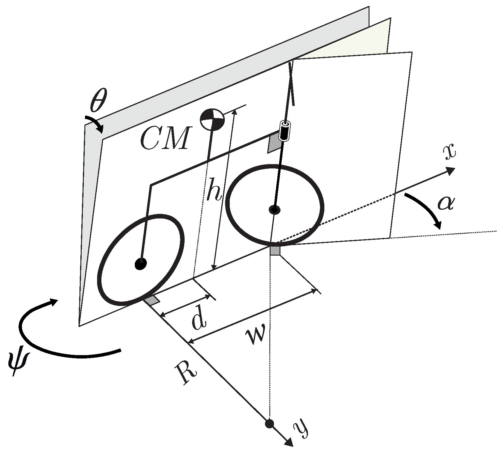
2.1. Dynamic Model
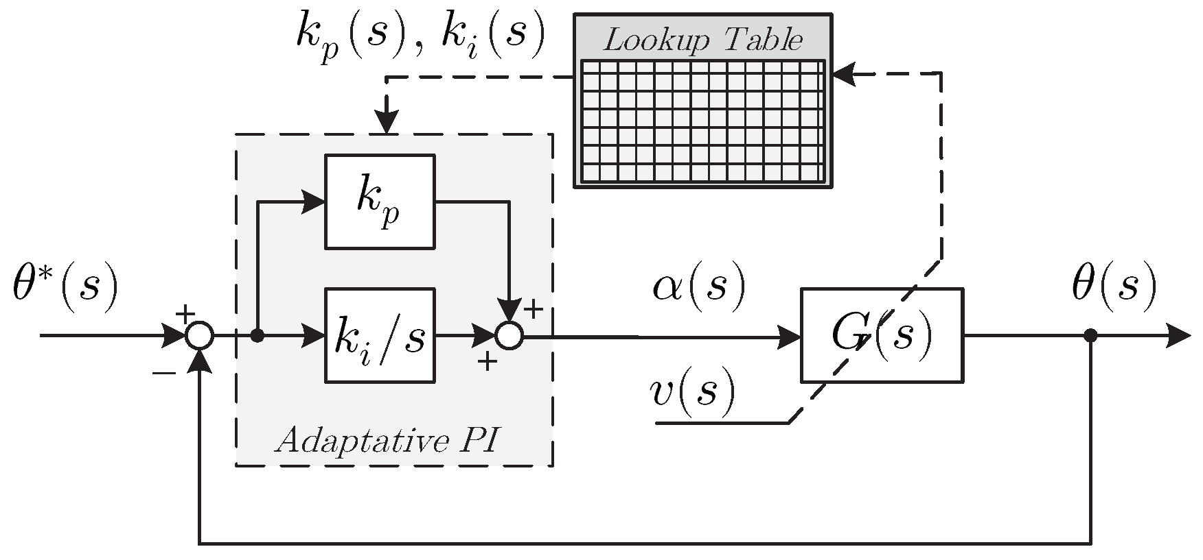
2.2. Control Law
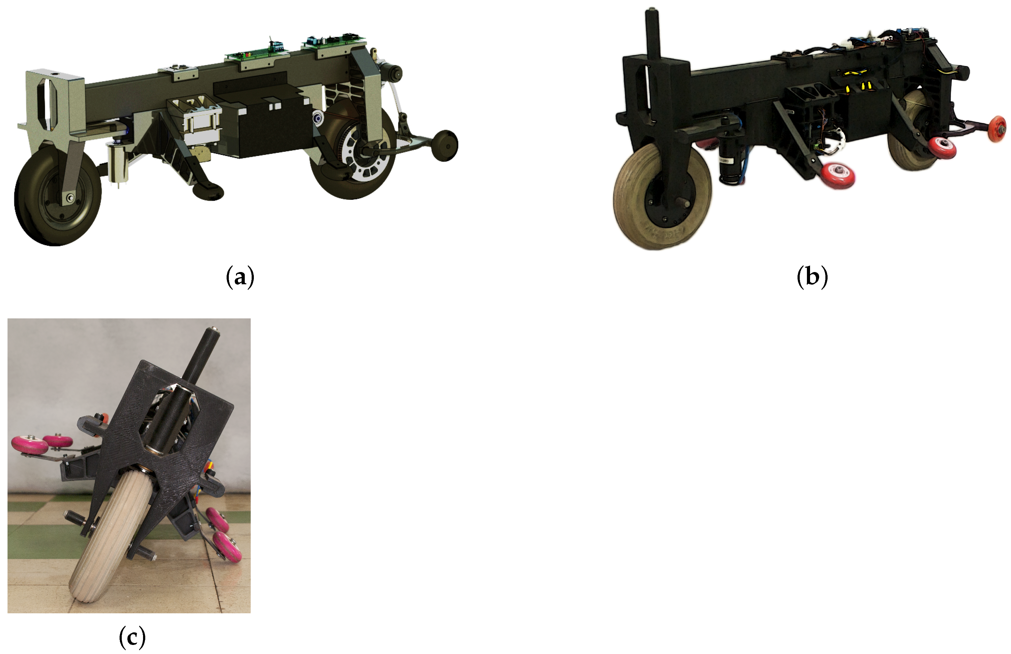
3. Description of the Experimental Prototype
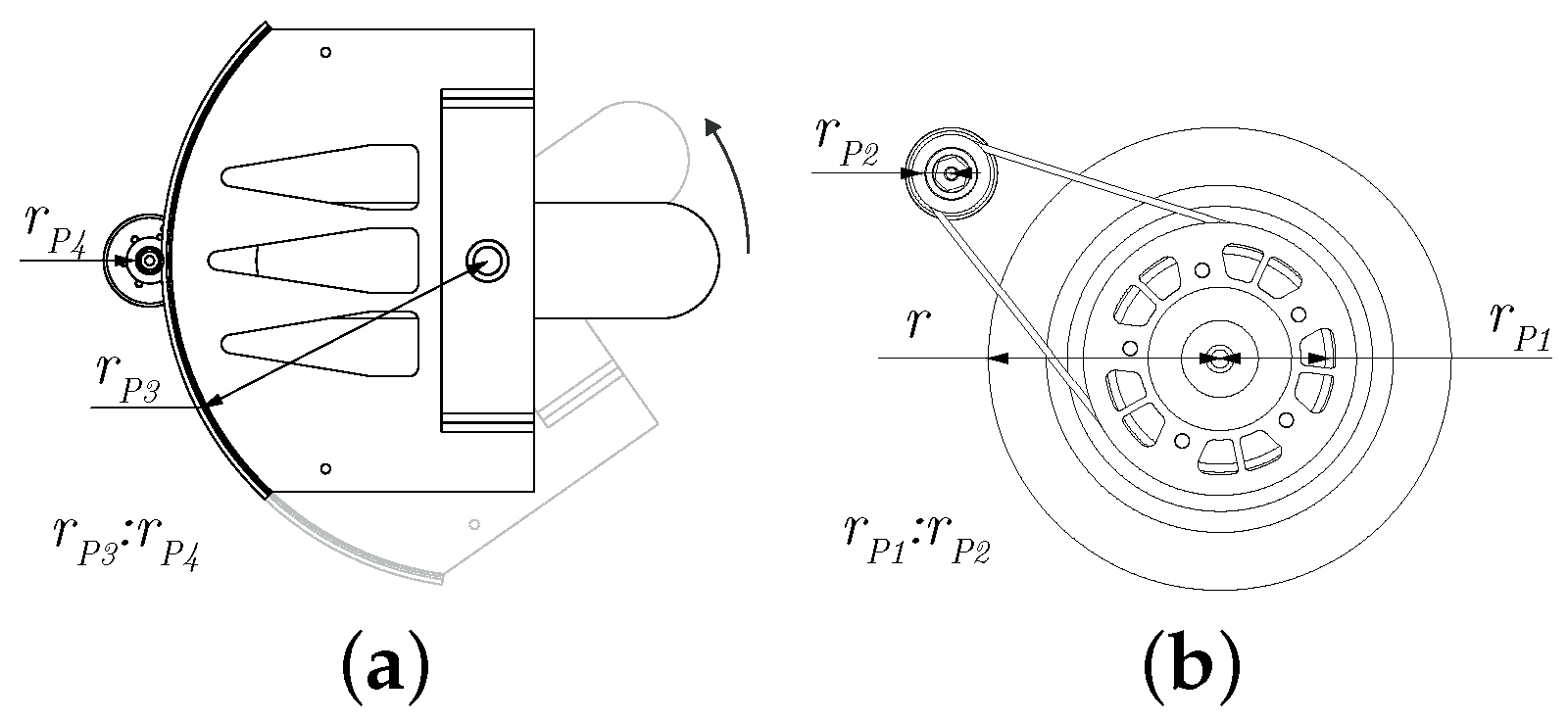
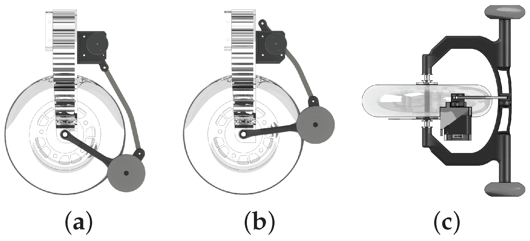
3.1. Mechanical Structure

| Parameter | Value [unit] |
|---|---|
| h | [m] |
| w | [m] |
| d | [m] |
| r | [m] |
| m | [kg] |
| [rad] | |
| [rad] |

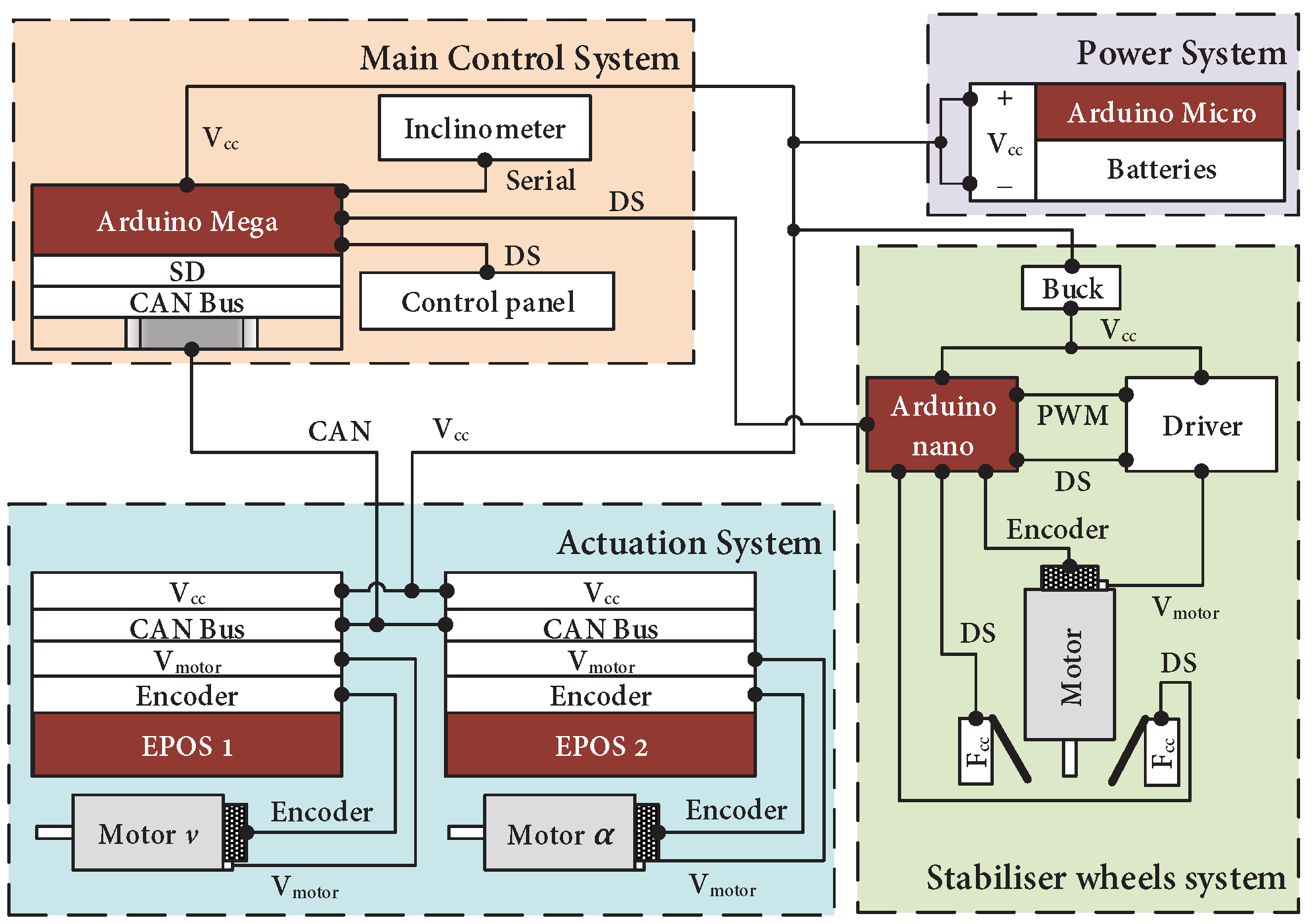
3.2. Electric/Electronic System
3.2.1. Power Supply
3.2.2. Actuation Systems
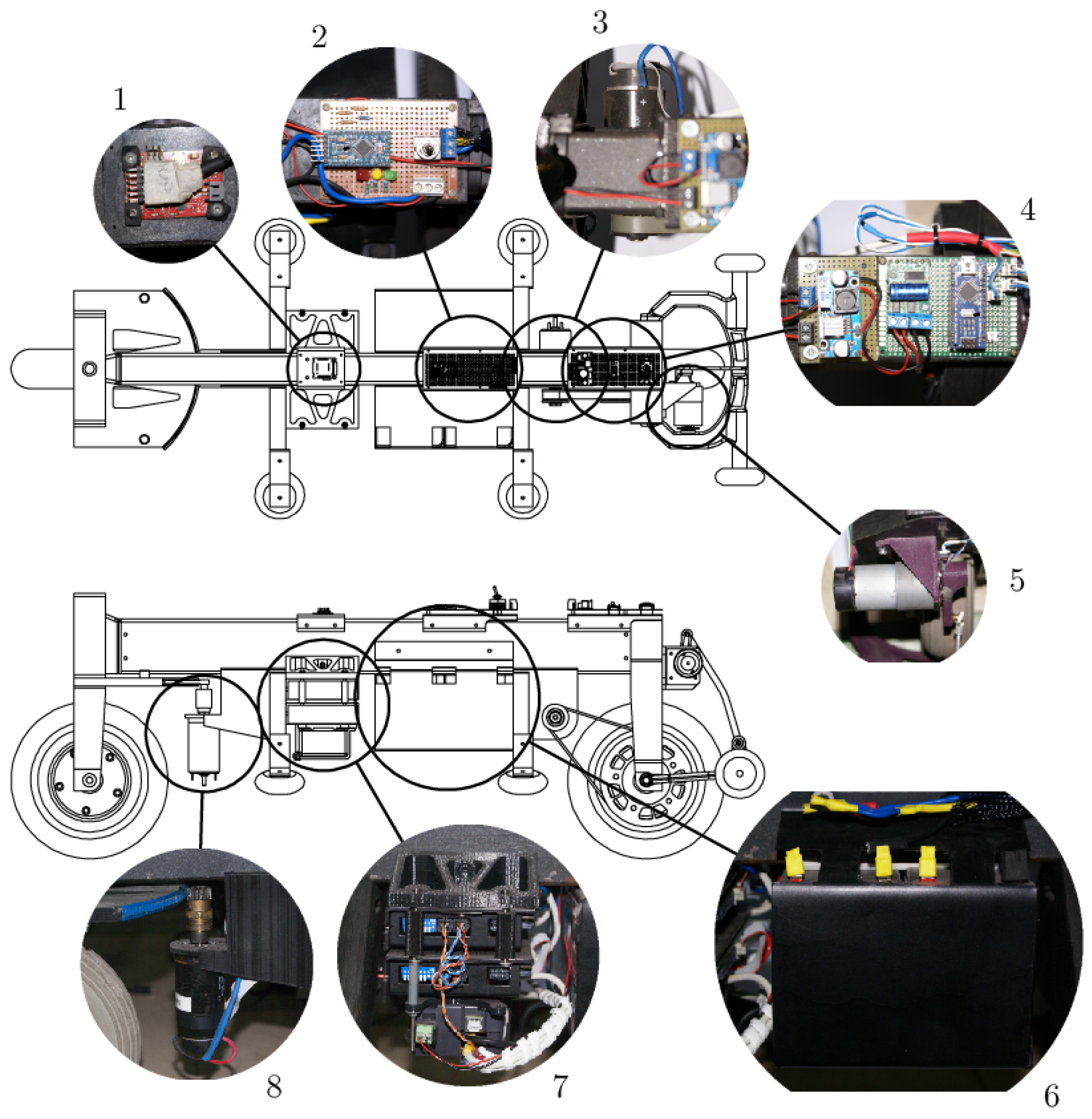
3.2.3. Control System
3.2.4. Stabilizer Wheel System
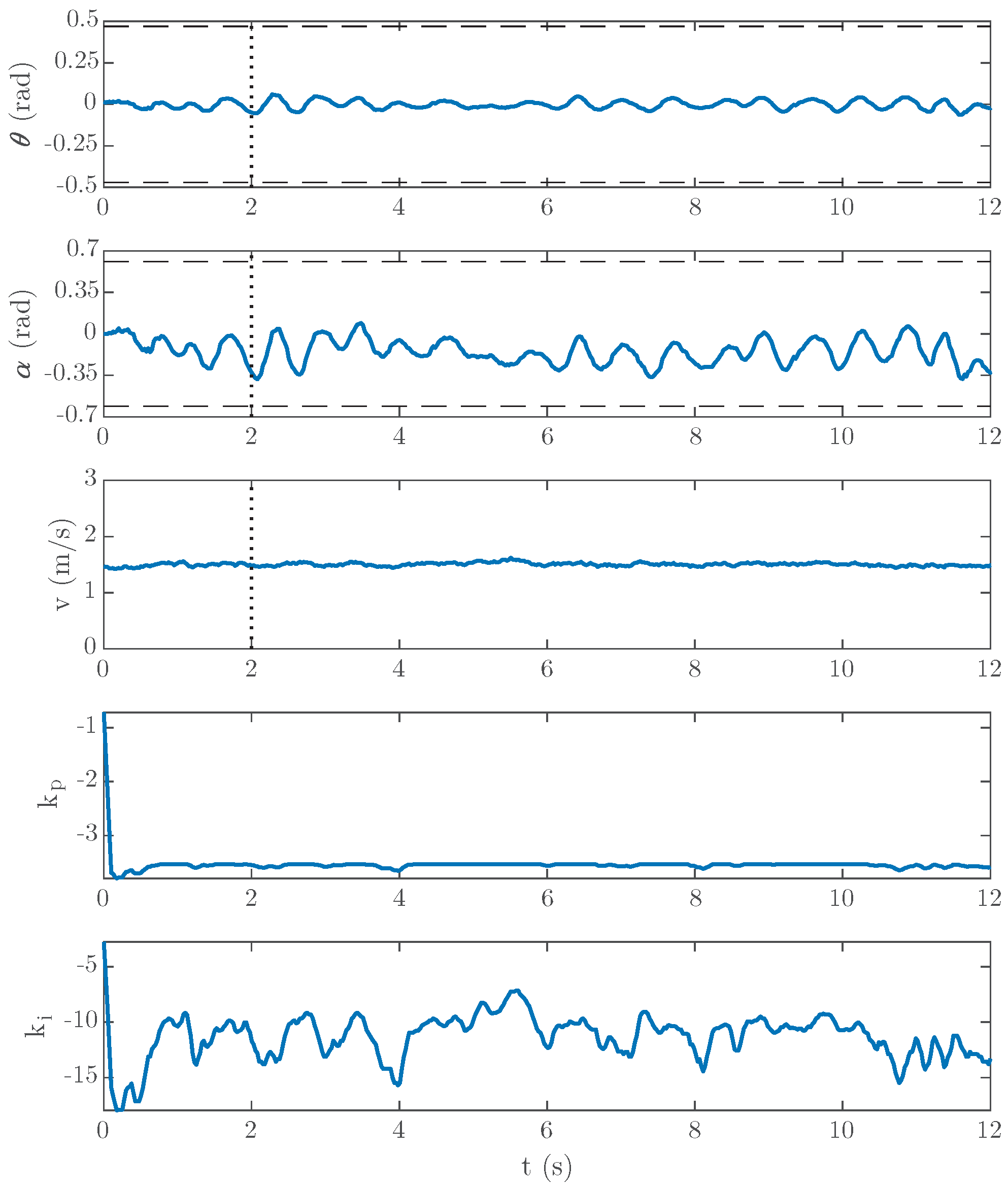
4. Performance Analysis
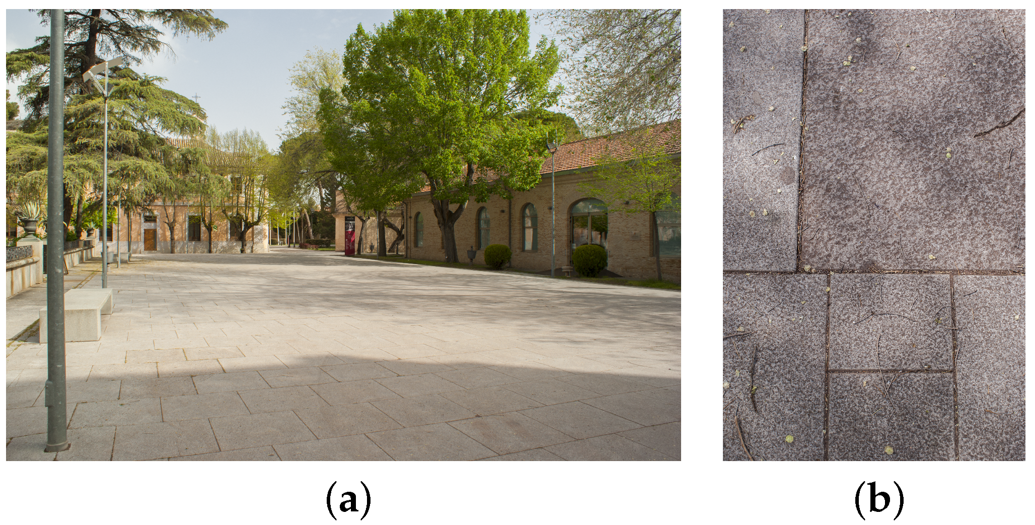
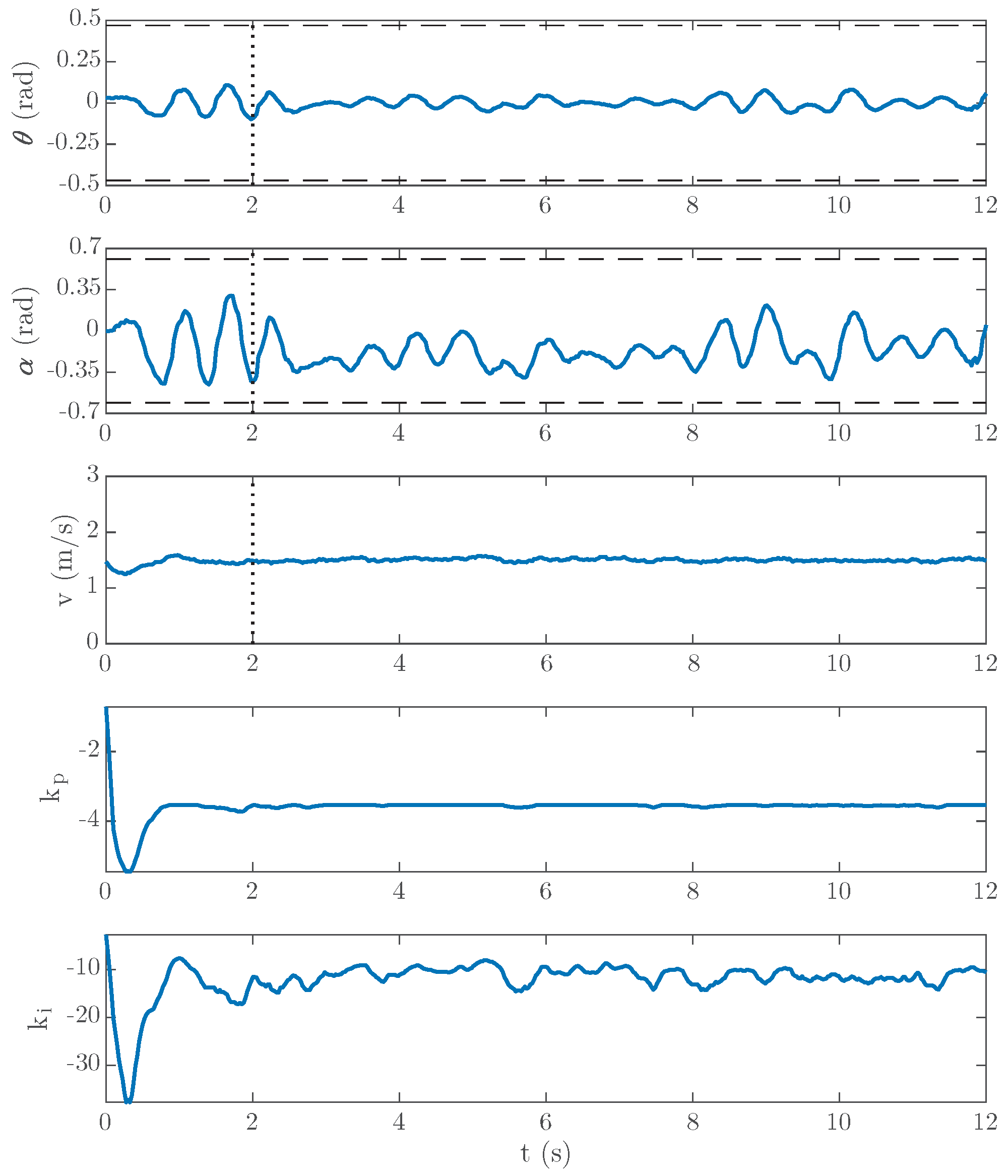
4.1. Tests Performed on Smooth Floor
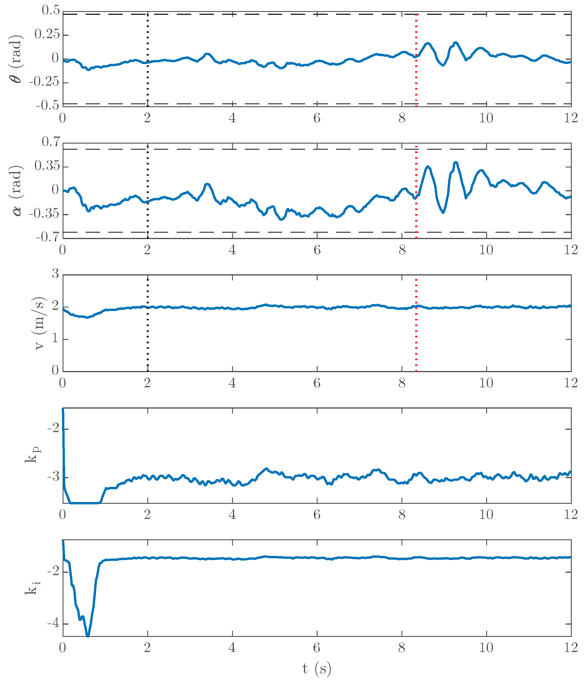
4.2. Tests Performed on Uneven Floor
4.3. Robustness Analysis
4.4. Discussion
- The stability performance, , is better at low speed.
- When the forward velocity increases, the required steering angle is smaller.
- The integral action of the controller is more required to maintain the lateral stability at low velocity and over rough terrain.
- The proportional action of the controller presents a similar behaviour at any speed.
- Based on the robustness analysis presented, the adaptive PI controller presents a robust behaviour when plant parameters vary within a reasonable range of .
5. Conclusions and Future Work
Author Contributions
Funding
Data Availability Statement
Conflicts of Interest
References
- Xiong, R.; Kim, J.; Shen, W.; Lv, C.; Li, H.; Zhu, X.; Zhao, W.; Gao, B.; Guo, H.; Zhang, C.; et al. Key technologies for electric vehicles. Green Energy Intell. Transp. 2022, l1, 100041. [Google Scholar] [CrossRef]
- Chen, C.; Xiong, R.; Yang, R.; Li, H. A novel data-driven method for mining battery open-circuit voltage characterization. Green Energy Intell. Transp. 2022, 1, 100001. [Google Scholar] [CrossRef]
- Shao, L.; Karci, A.E.H.; Tavernini, D.; Sorniotti, A.; Cheng, M. Design approaches and control strategies for energy-efficient electric machines for electric vehicles—A review. IEEE Access 2020, 8, 116900–116913. [Google Scholar] [CrossRef]
- Medaglia, A.; Wilches-Mogollon, M.; Sarmiento, O.; Montes, F.; Guzman, L.; Sanchez-Silva, M.; Menezes, R.; Hidalgo, D.; Parra, K.; Useche, A.; et al. Towards Intelligent Dynamics of an Active Transport System for Biking. R. Acad. Eng. 2022. [Google Scholar]
- Stilo, L.; Segura-Velandia, D.; Lugo, H.; Conway, P.P.; West, A.A. Electric bicycles, next generation low carbon transport systems: A survey. Transp. Res. Interdiscip. Perspect. 2021, 10, 100347. [Google Scholar] [CrossRef]
- Ma, Y.; Chen, J.; Zhu, X.; Xu, Y. Lateral stability integrated with energy efficiency control for electric vehicles. Mech. Syst. Signal Process. 2019, 127, 1–15. [Google Scholar] [CrossRef]
- Rodriguez-Rosa, D.; Payo-Gutierrez, I.; Castillo-Garcia, F.J.; Gonzalez-Rodriguez, A.; Perez-Juarez, S. Improving Energy Efficiency of an Autonomous Bicycle with Adaptive Controller Design. Sustainability 2017, 9, 866. [Google Scholar] [CrossRef]
- Manrique-Escobar, C.A.; Pappalardo, C.M.; Guida, D. On the analytical and computational methodologies for modelling two-wheeled vehicles within the multibody dynamics framework: A systematic literature review. J. Appl. Comput. Mech. 2022, 8, 153–181. [Google Scholar]
- Ni, T.; Li, W.; Zhao, D.; Kong, Z. Road profile estimation using a 3D sensor and intelligent vehicle. Sensors 2020, 20, 3676. [Google Scholar] [CrossRef]
- Wang, D.; Tahmasebi, K.N.; Chen, D. Integrated Control of Steering and Braking for Effective Collision Avoidance with Autonomous Emergency Braking in Automated Driving. In Proceedings of the 2022 30th Mediterranean Conference on Control and Automation (MED), Vouliagmeni, Greece, 28 June–1 July 2022; IEEE: Piscataway, NJ, USA, 2022; pp. 945–950. [Google Scholar]
- Tahir, M.N.; Mäenpää, K.; Sukuvaara, T.; Leviäkangas, P. Deployment and analysis of cooperative intelligent transport system pilot service alerts in real environment. IEEE Open J. Intell. Transp. Syst. 2021, 2, 140–148. [Google Scholar] [CrossRef]
- Vu, V.; Warg, F.; Thorsén, A.; Ursing, S.; Sunnerstam, F.; Holler, J.; Bergenhem, C.; Cosmin, I. Minimal Risk Manoeuvre Strategies for Cooperative and Collaborative Automated Vehicles. In Proceedings of the 2023 53rd Annual IEEE/IFIP International Conference on Dependable Systems and Networks Workshops (DSN-W), Porto, Portugal, 27–30 June 2023; IEEE: Piscataway, NJ, USA, 2023; pp. 116–123. [Google Scholar]
- Koenders, E.; Vreeswijk, J. Cooperative infrastructure. In Proceedings of the 2008 IEEE Intelligent Vehicles Symposium, Eindhoven, The Netherlands, 4–6 June 2008; IEEE: Piscataway, NJ, USA, 2008; pp. 721–726. [Google Scholar]
- Malizia, F.; Blocken, B. Bicycle aerodynamics: History, state-of-the-art and future perspectives. J. Wind. Eng. Ind. Aerodyn. 2020, 200, 104134. [Google Scholar] [CrossRef]
- Meijaard, J.; Papadopoulos, J.M.; Ruina, A.; Schwab, A. Supplementary appendices. Linearized dynamics equations for the balance and steer of a bicycle: A benchmark and review. Proc. R. Soc. Ser. 2007. [Google Scholar] [CrossRef]
- Whipple, F.J. The stability of the motion of a bicycle. Q. J. Pure Appl. Math. 1899, 30, 312–384. [Google Scholar]
- Carvallo, E. Théorie du mouvement du monocycle et de la bicyclette. L’Ecole Polytech. 1900. [Google Scholar]
- Boussinesq, J. Aperçu sur la théorie de la bicyclette. J. MathÉMatiques Pures AppliquÉEs 1899, 5, 117–136. [Google Scholar]
- Rill, G. Sophisticated but quite simple contact calculation for handling tire models. Multibody Syst. Dyn. 2019, 45, 131–153. [Google Scholar] [CrossRef]
- Schwab, A.L.; Meijaard, J.P. A review on bicycle dynamics and rider control. Veh. Syst. Dyn. 2013, 51, 1059–1090. [Google Scholar] [CrossRef]
- Carputo, F.; D’Andrea, D.; Risitano, G.; Sakhnevych, A.; Santonocito, D.; Farroni, F. A neural-network-based methodology for the evaluation of the center of gravity of a motorcycle rider. Vehicles 2021, 3, 377–389. [Google Scholar] [CrossRef]
- Hu, J.; Rakheja, S.; Zhang, Y. Real-time estimation of tire–road friction coefficient based on lateral vehicle dynamics. Proc. Inst. Mech. Eng. Part J. Automob. Eng. 2020, 234, 2444–2457. [Google Scholar] [CrossRef]
- Manrique-Escobar, C.A.; Pappalardo, C.M.; Guida, D. A multibody system approach for the systematic development of a closed-chain kinematic model for two-wheeled vehicles. Machines 2021, 9, 245. [Google Scholar] [CrossRef]
- Wang, J.J. Simulation studies of inverted pendulum based on PID controllers. Simul. Model. Pract. Theory 2011, 19, 440–449. [Google Scholar] [CrossRef]
- Dang, Q.V.; Allouche, B.; Vermeiren, L.; Dequidt, A.; Dambrine, M. Design and implementation of a robust fuzzy controller for a rotary inverted pendulum using the Takagi-Sugeno descriptor representation. In Proceedings of the 2014 IEEE Symposium on Computational Intelligence in Control and Automation (CICA), Orlando, FL, USA, 9–12 December 2014; IEEE: Piscataway, NJ, USA, 2014; pp. 1–6. [Google Scholar]
- Wei, E.; Li, T.; Li, J.; Hu, Y.; Li, Q. Neural network-based adaptive dynamic surface control for inverted pendulum system. In Foundations and Practical Applications of Cognitive Systems and Information Processing; Springer: Berlin/Heidelberg, Germany, 2014; pp. 695–704. [Google Scholar]
- Gupta, N.K.; Ambikapathy, A. Self-Balancing Bicycle using Reaction Wheel. Int. J. Eng. Sci. 2019, 21405, 21402–21407. [Google Scholar]
- Zheng, X.; Zhu, X.; Chen, Z.; Sun, Y.; Liang, B.; Wang, T. Dynamic modeling of an unmanned motorcycle and combined balance control with both steering and double CMGs. Mech. Mach. Theory 2022, 169, 104643. [Google Scholar] [CrossRef]
- Yang, C.; Murakami, T. Full-speed range self-balancing electric motorcycles without the handlebar. IEEE Trans. Ind. Electron. 2015, 63, 1911–1922. [Google Scholar] [CrossRef]
- Yamakita, M.; Utano, A.; Sekiguchi, K. Experimental study of automatic control of bicycle with balancer. In Proceedings of the 2006 IEEE/RSJ International Conference on Intelligent Robots and Systems, Beijing, China, 9–15 October 2006; IEEE: Piscataway, NJ, USA, 2006; pp. 5606–5611. [Google Scholar]
- Keo, L.; Yamakita, M. Controlling balancer and steering for bicycle stabilization. In Proceedings of the 2009 IEEE/RSJ International Conference on Intelligent Robots and Systems, St. Louis, MO, USA, 10–15 October 2009; IEEE: Piscataway, NJ, USA, 2009; pp. 4541–4546. [Google Scholar]
- Keo, L.; Yoshino, K.; Kawaguchi, M.; Yamakita, M. Experimental results for stabilizing of a bicycle with a flywheel balancer. In Proceedings of the 2011 IEEE International Conference on Robotics and Automation, Shanghai, China, 9–13 May 2011; IEEE: Piscataway, NJ, USA, 2011; pp. 6150–6155. [Google Scholar]
- Kawaguchi, M.; Yamakita, M. Stabilizing of bike robot with variable configured balancer. In Proceedings of the SICE Annual Conference 2011, Tokyo, Japan, 13–18 September 2011; IEEE: Piscataway, NJ, USA, 2011; pp. 1057–1062. [Google Scholar]
- Yeh, T.J.; Lu, H.; Tseng, P. Balancing Control of a Self-driving Bicycle. In Proceedings of the 16th International Conference on Informatics in Control, Automation and Robotics, Prague, Czech Republic, 29–31 July 2019; Volume 2, pp. 34–41. [Google Scholar] [CrossRef]
- Limebeer, D.J.; Sharp, R.S. Bicycles, motorcycles, and models. IEEE Control. Syst. 2006, 26, 34–61. [Google Scholar]
- Anjumol, M.; Jisha, V. Optimal stabilization and straight line tracking of an electric bicycle. In Proceedings of the 2014 International Conference on Power Signals Control and Computations (EPSCICON), Thrissur, India, 6–11 January 2014; IEEE: Piscataway, NJ, USA, 2014; pp. 1–6. [Google Scholar]
- Yuan, J.; Chen, H.; Sun, F.; Huang, Y. Trajectory planning and tracking control for autonomous bicycle robot. Nonlinear Dyn. 2014, 78, 421–431. [Google Scholar] [CrossRef]
- Yuan, J.; Zhang, J.; Ding, S. Pseudospectral motion planning for autonomous bicycles. In Proceedings of the 2015 IEEE International Conference on Advanced Intelligent Mechatronics (AIM), Busan, Republic of Korea, 7–11 July 2015; IEEE: Piscataway, NJ, USA, 2015; pp. 482–487. [Google Scholar]
- Zhuang, W.; Zhang, R.; Su, X.; Huang, Y. Research on the Lateral Balance Control of a Bicycle Robot. In Proceedings of the 2019 International Conference on Robotics, Intelligent Control and Artificial Intelligence, Beijing, China, 19–22 April 2019; pp. 744–750. [Google Scholar]
- Hatano, R.; Tani, T.; Iwase, M. Stability analysis and autonomous stabilization control of a bicycle based on a three-dimensional detailed physical model. In Proceedings of the IECON 2016-42nd Annual Conference of the IEEE Industrial Electronics Society, Florence, Italy, 23–26 October 2016; IEEE: Piscataway, NJ, USA, 2016; pp. 324–329. [Google Scholar]
- Tanaka, Y.; Murakami, T. A study on straight-line tracking and posture control in electric bicycle. IEEE Trans. Ind. Electron. 2008, 56, 159–168. [Google Scholar] [CrossRef]
- Defoort, M.; Murakami, T. Sliding-mode control scheme for an intelligent bicycle. IEEE Trans. Ind. Electron. 2009, 56, 3357–3368. [Google Scholar] [CrossRef]
- Yamaguchi, T.; Shibata, T.; Murakami, T. Self-sustaining approach of electric bicycle by acceleration control based backstepping. In Proceedings of the IECON 2007-33rd Annual Conference of the IEEE Industrial Electronics Society, Taipei, Taiwan, 5–8 November 2007; IEEE: Piscataway, NJ, USA, 2007; pp. 2610–2614. [Google Scholar]
- Defoort, M.; Murakami, T. Second order sliding mode control with disturbance observer for bicycle stabilization. In Proceedings of the 2008 IEEE/RSJ International Conference on Intelligent Robots and Systems, Nice, France, 22–26 September 2008; IEEE: Piscataway, NJ, USA, 2008; pp. 2822–2827. [Google Scholar]
- Rodriguez-Rosa, D.; Payo-Gutierrez, I.; Gonzalez-Lucena, I.; Gonzalez-Rodriguez, A.; Castillo-Garcia, F.J.; Gonzalez-Rodriguez, A. Controlador proporcional-integral adaptativo para el ahorro energético en bicicletas autónomas. DYNA 2014, 89, 656–664. [Google Scholar] [CrossRef]
- Hashemnia, S.; Shariat Panahi, M.; Mahjoob, M.J. Unmanned bicycle balancing via Lyapunov rule-based fuzzy control. Multibody Syst. Dyn. 2014, 31, 147–168. [Google Scholar] [CrossRef]
- Dao, T.K.; Chen, C.K. Sliding-mode control for the roll-angle tracking of an unmanned bicycle. Veh. Syst. Dyn. 2011, 49, 915–930. [Google Scholar] [CrossRef]
- Keo, L.; Masaki, Y. Trajectory control for an autonomous bicycle with balancer. In Proceedings of the 2008 IEEE/ASME International Conference on Advanced Intelligent Mechatronics, Xi’an, China, 2–5 July 2008; IEEE: Piscataway, NJ, USA, 2008; pp. 676–681. [Google Scholar]
- Getz, N.H.; Marsden, J.E. Control for an autonomous bicycle. In Proceedings of the 1995 IEEE International Conference on Robotics and Automation, Nagoya, Aichi, Japan, 21–27 May 1995; IEEE: Piscataway, NJ, USA, 1995; Volume 2, pp. 1397–1402. [Google Scholar]
- Baquero-Suárez, M.; Cortés-Romero, J.; Arcos-Legarda, J.; Coral-Enriquez, H. A robust two-stage active disturbance rejection control for the stabilization of a riderless bicycle. Multibody Syst. Dyn. 2019, 45, 7–35. [Google Scholar] [CrossRef]
- Xiong, C.; Huang, Z.; Gu, W.; Pan, Q.; Liu, Y.; Li, X.; Wang, E. Static balancing of robotic bicycle through nonlinear modeling and control. In Proceedings of the 2018 3rd International Conference on Robotics and Automation Engineering (ICRAE), Guangzhou, China, 17–19 November 2018; IEEE: Piscataway, NJ, USA, 2018; pp. 24–28. [Google Scholar]
- Tanaka, Y.; Murakami, T. Self sustaining bicycle robot with steering controller. In Proceedings of the 8th IEEE International Workshop on Advanced Motion Control, 2004. AMC’04, Kawasaki, Japan, 25–28 March 2004; IEEE: Piscataway, NJ, USA, 2004; pp. 193–197. [Google Scholar]
- Li, C.; Xie, Y.F.; Wang, G.; Zeng, X.F.; Jing, H. Lateral stability regulation of intelligent electric vehicle based on model predictive control. J. Intell. Connect. Veh. 2021, 4, 104–114. [Google Scholar] [CrossRef]
- Wen, G.; Sjöberg, J. Lateral control of a self-driving bike. In Proceedings of the 2022 IEEE International Conference on Vehicular Electronics and Safety (ICVES), Bogota, Colombia, 14–16 November 2022; IEEE: Piscataway, NJ, USA, 2022; pp. 1–6. [Google Scholar]
- Chu, T.; Chen, C. Modelling and model predictive control for a bicycle-rider system. Veh. Syst. Dyn. 2018, 56, 128–149. [Google Scholar] [CrossRef]
- Coppola, A.; Lui, D.G.; Petrillo, A.; Santini, S. Eco-driving control architecture for platoons of uncertain heterogeneous nonlinear connected autonomous electric vehicles. IEEE Trans. Intell. Transp. Syst. 2022, 23, 24220–24234. [Google Scholar] [CrossRef]


| Work | Control Approach Description | Tuning Method | Energy Optimisation | |
|---|---|---|---|---|
| Included? | Can Be? | |||
| [46] | Fuzzy control | Lyapunov based | No | No |
| [47] | Sliding-mode control | Error minimisation | No | Yes |
| [48] | Output-zeroing control | Algebraic identification | No | No |
| [49] | Coupling PD controllers | Not defined | No | No |
| [50] | Active disturbance rejection | Algebraic identification | No | No |
| [51] | LQR controller | Minimising target function | No | Yes |
| [52] | PD controller | Frequency domain tuning | No | No |
| [53] | Model predictive control | Minimising target function | No | Yes |
| [54] | LQR + P controller | Minimising target function | No | Yes |
| [55] | Model predictive control | Minimising target function | No | Yes |
| Uncertainty Range | 0% (Nominal) | ||||
|---|---|---|---|---|---|
| h (m) | 0.0950 | 0.1425 | 0.1900 | 0.2375 | 0.2850 |
| w (m) | 0.3500 | 0.5250 | 0.7000 | 0.8750 | 1.0500 |
| d (m) | 0.1550 | 0.2325 | 0.3100 | 0.3875 | 0.4650 |
| Uncertainty Range | 0% (Nominal) | ||||
|---|---|---|---|---|---|
| (v = 1.5 m/s2) | 5.0930 | 5.2184 | 5.3265 | 5.4367 | 5.5369 |
| (v = 2.0 m/s2) | 6.8306 | 6.5465 | 6.3369 | 6.1680 | 6.0306 |
| Experiment | 1 | 2 | 3 | 4 |
|---|---|---|---|---|
| Terrain | smooth | smooth | rough | rough |
| 0 | 0.47 | 0 | 0 | |
| (m/s) | 1.5 | 2.2 | 1.5 | 2.0 |
| 0.2507 | 3.1854 | 0.3558 | 0.5223 | |
| 1.8325 | 4.9026 | 2.2986 | 2.0262 | |
| 18.0957 | 26.1462 | 17.9413 | 23.7291 | |
Disclaimer/Publisher’s Note: The statements, opinions and data contained in all publications are solely those of the individual author(s) and contributor(s) and not of MDPI and/or the editor(s). MDPI and/or the editor(s) disclaim responsibility for any injury to people or property resulting from any ideas, methods, instructions or products referred to in the content. |
© 2024 by the authors. Licensee MDPI, Basel, Switzerland. This article is an open access article distributed under the terms and conditions of the Creative Commons Attribution (CC BY) license (https://creativecommons.org/licenses/by/4.0/).
Share and Cite
Rodríguez-Rosa, D.; Martín-Parra, A.; García-Vanegas, A.; Moya-Fernández, F.; Payo-Gutiérrez, I.; Castillo-García, F.J. Vertical Balance of an Autonomous Two-Wheeled Single-Track Electric Vehicle. Technologies 2024, 12, 76. https://doi.org/10.3390/technologies12060076
Rodríguez-Rosa D, Martín-Parra A, García-Vanegas A, Moya-Fernández F, Payo-Gutiérrez I, Castillo-García FJ. Vertical Balance of an Autonomous Two-Wheeled Single-Track Electric Vehicle. Technologies. 2024; 12(6):76. https://doi.org/10.3390/technologies12060076
Chicago/Turabian StyleRodríguez-Rosa, David, Andrea Martín-Parra, Andrés García-Vanegas, Francisco Moya-Fernández, Ismael Payo-Gutiérrez, and Fernando J. Castillo-García. 2024. "Vertical Balance of an Autonomous Two-Wheeled Single-Track Electric Vehicle" Technologies 12, no. 6: 76. https://doi.org/10.3390/technologies12060076
APA StyleRodríguez-Rosa, D., Martín-Parra, A., García-Vanegas, A., Moya-Fernández, F., Payo-Gutiérrez, I., & Castillo-García, F. J. (2024). Vertical Balance of an Autonomous Two-Wheeled Single-Track Electric Vehicle. Technologies, 12(6), 76. https://doi.org/10.3390/technologies12060076