Fault Detection of Wheelset Bearings through Vibration-Sound Fusion Data Based on Grey Wolf Optimizer and Support Vector Machine

Abstract

This study aims to detect faults in wheelset bearings by analyzing vibration-sound fusion data, proposing a novel method based on Grey Wolf Optimizer (GWO) and Support Vector Machine (SVM). Wheelset bearings play a vital role in transportation. However, malfunctions in the bearing might result in extensive periods of inactivity and maintenance, disrupting supply chains, increasing operational costs, and causing delays that affect both businesses and consumers. Fast fault identification is crucial for minimizing maintenance expenses. In this paper, we proposed a new integration of GWO for optimizing SVM hyperparameters, specifically tailored for handling sound-vibration signals in fault detection. We have developed a new fault detection method that efficiently processes fusion data and performs rapid analysis and prediction within 0.0027 milliseconds per data segment, achieving a test accuracy of 98.3%. Compared to the SVM and neural network models built in MATLAB, the proposed method demonstrates superior detection performance. Overall, the GWO-SVM-based method proposed in this study shows significant advantages in fault detection of wheelset bearing vibrations, providing an efficient and reliable solution that is expected to reduce maintenance costs and improve the operational efficiency and reliability of equipment.

1. Introduction

Bearings play a crucial role in transportation, with their operational safety and reliability directly impacting logistics efficiency and economic benefits. The wheelset bearings are key components that bear significant loads and operate in complex environments. Over extended periods of use, these bearings are prone to various faults. Therefore, timely and effective detection of wheelset bearings faults is essential for ensuring the safety of transportation.

The primary objective of bearing fault diagnostics is to detect probable defects by examining diverse data. Vibration data is a widely utilized technique for diagnosing bearing failures, as these faults generally result in anomalous vibration characteristics. There are three predominant analysis methods: time domain analysis, frequency domain analysis, and time-frequency analysis. Time domain analysis involves the examination of the time waveform to identify impact signals and periodic components. The statistical properties, such as mean, variance, peak value, kurtosis, and skewness, can potentially reveal changes in the vibration signal [1]. The analysis typically involves computing these features from segmented windows of the vibration signal and monitoring their trends over time. Substantial departures from baseline values can suggest the existence and intensity of bearing faults [2,3,4]. Time domain analysis is a straightforward and efficient method for detecting bearing faults; however, it may not offer as much comprehensive diagnostic information as frequency domain techniques [2]. Frequency domain analysis involves applying a Fourier transform to convert signals in the time domain into signals in the frequency domain in order to identify and analyze certain frequency components [5]. Chen et al. [6] introduced power function-based Gini indices II and III (PFGI2 and PFGI3), and through mathematical derivation and experimental validation using envelope analysis in the frequency domain, demonstrated their superior sparsity quantification capabilities and fault feature characterization performance in bearing condition monitoring. Power Spectral Density (PSD) is a measure of the power distribution of a signal over different frequencies; it displays the amplitude of different frequency components and is commonly used to detect specific defects in bearings, such as defects in the outer ring, inner ring, or rolling elements [7]. Chen et al. [8] proposed two new blind deconvolution methods using the modified smoothness index (MSI) in the time and frequency domains for squared envelope applications, effectively enhancing sparse features for rolling bearing fault diagnosis and demonstrating excellent diagnostic performance and robustness in experiments. Time-frequency analysis involves the application of techniques that incorporate both time and frequency data, such as the Short-Time Fourier Transform (STFT) and Wavelet Transform [9,10]. These methods are able to capture the transitory properties of a signal with more accuracy [11].

Additionally, sound signal analysis is becoming more crucial in diagnosing bearing faults, as variations in sound signals might indicate changes in the operating conditions of the bearing. The conventional techniques used are analogous to the analysis of vibration data, encompassing time domain analysis, frequency domain analysis, and time-frequency domain analysis. Two more methods exist: sound pressure level (SPL) analysis and sound signature recognition. SPL analysis is an effective technique for diagnosing bearing faults by analyzing sound emissions from bearings. The main sources of bearing noise are vibrations from the inner ring and rolling elements (balls or rollers) and as a bearing enters the failure stage, there is a rise in SPL of 12–16 dB over the baseline level, accompanied by a change in sound quality [12,13]. SPL analysis includes three techniques: time waveform analysis, frequency spectrum analysis and time-frequency domain analysis [2,13]. Sound signature recognition in bearing fault detection involves utilizing sound signal analysis techniques to identify and diagnose bearing faults. This approach captures and analyzes the sound signals generated by bearings during operation, identifying abnormal patterns and features that indicate the bearing’s health status. Advanced signal processing techniques such as Fast Fourier Transform (FFT) [14], Wavelet Transform [10], Empirical Mode Decomposition [15], and Hilbert Transform are commonly used to extract fault features from noisy sound data [16,17,18,19,20].

Nevertheless, there are limitations when it comes to evaluating individual vibration signals or sound signals. For example, the presence of machinery might influence vibrations, making it difficult to discern certain defect features. In a similar manner, background noise has the potential to disrupt signals by concealing important fault characteristics. In data fusion, vibration and sound signals provide complementary information about machine condition, and data fusion has the potential to greatly enhance the effectiveness and dependability of bearing fault diagnosis systems, offering robust assistance for equipment preventative maintenance and fault prediction [21,22,23,24].

To enhance the accuracy and reliability of bearing faults detection systems, research investigations highlight the significance of data fusion approaches, which involve merging information from multiple sensors. Wan et al. [25] proposed a fusion multiscale convolutional neural network (F-MSCNN) method that processes raw sound and vibration signals to achieve high accuracy and stable fault diagnosis of rolling bearings under varying operating speeds. Shi et al. [26] proposed a two-stage sound-vibration signal fusion algorithm that combines and weights fault features from multiple sound measurement points, extracts features using empirical mode decomposition and kurtosis superposition, and then unifies sampling frequencies to fuse sound and vibration signals again, achieving weak fault detection in rolling bearings. This method significantly improves fault feature detection accuracy and signal-to-noise ratio, aiding in the status monitoring of bearing systems. Duan et al. [27] provided a comprehensive review of multi-sensor information fusion for rolling bearings, highlighting the significance of combining data from diverse sensors for improved fault diagnosis capabilities. Wang et al. [28] conducted a study on bearing fault diagnosis using vibro-sound data fusion and a 1D-CNN network, demonstrating the benefits of integrating vibration and sound information for enhanced fault detection. Gu et al. [29] introduced an enhanced SE-ResNet sound-vibration fusion method for rolling bearing fault diagnosis, integrating various techniques to effectively process sound-vibration signals. By integrating vibration and sound data, a comprehensive method for detecting bearing faults is achieved. This approach combines the advantages of both signal types, resulting in a more precise and detailed depiction of the system’s status. Researchers have successfully built sophisticated models that incorporate vibration and sound data using modern computational approaches such as deep learning, feature fusion, and adaptive signal processing. These models are used for precise problem identification in bearing systems. These studies highlight the significance of data fusion approaches in utilizing the combined benefits of vibration and sound inputs to improve the accuracy and effectiveness of bearing defect detection systems. However, these deep-learning-based methods need large datasets for training and they are not easily implemented for real-time detection.

In this study, we introduce a novel approach by integrating the Grey Wolf Optimizer (GWO) [30] with a Support Vector Machine (SVM) [31] to optimize hyperparameters, specifically tailored for real-time analysis of vibration-sound fusion data. Yan et al. proposed GWO-SVM for smart emotion recognition, they used the Radial Basis Function (RBF) kernel of SVM and achieved high accuracy in their research [32]. We extend their method with various SVM kernels and provide rapid failure detection by preprocessing fusion data from vibrations and sounds. Data segmentation facilitated analysis, enabling the model to generate predictions at a remarkable speed of 0.0027 milliseconds per segment. In addition, the linear SVM model that was fine-tuned using GWO achieved a testing accuracy of 98.3%, outperforming the SVM and neural network models built in MATLAB. Furthermore, this model demonstrated significant efficiency in runtime assessments, making it extremely suitable for real-world settings. The proposed GWO-SVM model shows advantages in detecting defects in wheelset bearings. The model’s capacity to generate real-time predictions and offer a comprehensive evaluation of the bearing’s condition can greatly diminish maintenance expenses and enhance the accessibility and effectiveness of wheelset bearings. This study underscores the potential of integrating advanced optimization algorithms with machine learning techniques to enhance fault detection capabilities, ultimately contributing to more robust and efficient transportation systems.

2. Methodology

The list of abbreviations are shown in

Table 1. Description of abbreviations.

Abbreviations	Description
CNN	Convolutional Neural Network
FFT	Fast Fourier Transform
GWO	Grey Wolf Optimizer
MFCC	Mel-Frequency Cepstral Coefficients
PCA	Principal Component Analysis
PSD	Power Spectral Density
RBF	Radial Basis Function
SPL	Sound Pressure Level
STFT	Short-Time Fourier Transform
SVM	Support Vector Machine

:

2.1. Overview of the Proposed Method

An overview of the proposed method is shown in Figure 1. The vibration signal is collected by accelerometers, which are located on the axle box cover in the bearing area at the end of the wheelset; and the sound signal is collected by microphone located on both sides of the bearing. This data set offers the vibration and sound data to efficiently identify bearing various faults.

Figure 1a shows the wheelset bearing. As shown in Figure 1b,c, FFT is utilized for analyzing vibration signals [14], whereas the Mel-Frequency Cepstral Coefficients (MFCC) are employed for analyzing sound signals [33]; split the data into different segments and then combine and integrate the characteristics of the two datasets by simply concatenating them; the model possesses the ability to rapidly examine every individual segment. The final stage involved the trained model making predictions for the score of each segment, as shown in Figure 1d.

2.2. The Description of the GWO-SVM Model

SVM have been widely applied for fault detection and diagnosis of bearings in rotating machinery. Pule et al. [34] proposed a method using principal component analysis (PCA) and SVM to achieve 97.4% accuracy in diagnosing bearing faults under varying speeds using vibration analysis. Yang et al. [35] introduced a triplet embedding-based method for classifying small sample rolling bearing fault datasets, achieving superior performance in fault diagnosis by using CNN for feature extraction and SVM for classification. Mo et al. [36] proposed a highly accurate (95.3%) and efficient (11.1608-s training time) method for diagnosing petrochemical rotating machinery bearing faults by combining ICEEMDAN-wavelet noise reduction, mutual dimensionless metrics, and MPGA-SVM, with further validation showing 97.1% accuracy on additional datasets.

In this paper, we adopted a fast detection GWO-SVM model by analyzing fusion data from multiple models to assess bearing failure, as shown in Figure 2

Step 1: Data preprocessing—Load the signals and extract their features and annotate their label.

Step 2: Initialize Wolves—Randomly generate the initial positions for the wolf pack, which are the candidate solutions for the SVM hyperparameters $C_{SVM}$ and $\gamma$, initialize the maximum number of iterations L and the number of search agents n.

Step 3: Evaluate fitness—Evaluate accuracy for each candidate using cross-validation. If $i\le n$:

• Select the current candidate i: Choose the i-th wolf from the pack.
• Train SVM model using current candidate: (1) Extract the SVM hyperparameters $C_{SVM}$ and $\gamma$ from the current candidate; (2) Initialize an SVM model with these parameters; (3) Train the SVM model on the training dataset.
• Evaluate the model on the validation set: (1) Use the validation dataset to predict outcomes; (2) Calculate the accuracy of the predictions, which represents the fitness of the current candidate
• Record the fitness value of the current candidate: Save the fitness value for the current candidate.
• Increment the index i: Move to the next candidate ($i=i+1$).
• Repeat Step 3: Continue evaluating the next candidate until all candidates are evaluated.

Step 4: Update ${\alpha }_{wolf}$, ${\beta }_{wolf}$, and ${\delta }_{wolf}$.—Based on the fitness values, select the top three candidates as the ${\alpha }_{wolf}$, ${\beta }_{wolf}$, and ${\delta }_{wolf}$.

Step 5: Update Wolves positions—Update the positions of all wolves in the pack using the positions of the ${\alpha }_{wolf}$, ${\beta }_{wolf}$, and ${\delta }_{wolf}$.

Step 6: Main loop—Continue iterating through Steps 3 to 5 until the maximum number of iterations L is reached or the algorithm converges.

Step 7: Final model training and testing—Use the best hyperparameters found during the optimization to train the SVM model on the entire training dataset. Evaluate the trained model on the test dataset.

Step 8: Format and display results—Format the evaluation results and print them. Save the trained model and results to a file.

Step 9: Save model—Save the trained SVM model to a specified file path.

Step 10: Measure runtime—Calculate and print the total runtime and the testing time.

2.2.1. Basic SVM Formula

The decision function for SVM:

$$f\left(x\right)=\sum _{i=1}^n{\alpha }_i{y}_{i}K(x_i,x)+b$$

(1)

where ${\alpha }_i$ is the Lagrange multiplier, $y_i$ is the label, $x_i$ is the support vector, $K(x_i,x)$ is the kernel function, and b is the bias term.

2.2.2. GWO Formulas

Updating parameter a:

$$a=2-2{\left({\displaystyle \frac{\mathrm{epoch}}{L}}\right)}^2$$

(2)

where epoch is the current iteration and L is the maximum number of iterations.

Calculating coefficients A and $C_{wolf}$:

$$\begin{array}{c}\hfill A=2·a·r_{{wolf}_{1-a}}\\ \hfill C_{wolf}=2·r_{{wolf}_2}\end{array}$$

(3)

where $r_{{wolf}_1}$ and $r_{{wolf}_2}$ are random numbers in the range $[0,1]$.

Updating the positions of the wolves:

$$\begin{array}{c}\hfill D_{\alpha }=|C_{wolf}·X_{\alpha }-X|\\ \hfill D_{\beta }=|C_{wolf}·X_{\beta }-X|\\ \hfill D_{\delta }=|C_{wolf}·X_{\delta }-X|\\ \hfill X_1=X_{\alpha }-A·D_{\alpha }\\ \hfill X_2=X_{\beta }-A·D_{\beta }\\ \hfill X_3=X_{\delta }-A·D_{\delta }\\ \hfill X_{\mathrm{new}}={\displaystyle \frac{X_1+X_2+X_3}{3}}\end{array}$$

(4)

Among them:

-

D represents the distance between the current wolf and the ${\alpha }_{wolf}$, ${\beta }_{wolf}$, and ${\delta }_{wolf}$.

-

$X_{\alpha ,\beta ,\delta }$ is the position of the ${\alpha }_{wolf}$, ${\beta }_{wolf}$, and ${\delta }_{wolf}$, representing the best solution found so far.

-

$X_{\mathrm{new}}$ is the updated position of the wolf, the elements in $X_{\mathrm{new}}$ are essentially combinations of SVM hyperparameters, optimized through the GWO process to find the best parameter settings.

2.2.3. GWO Algorithm Steps

Linear Kernel function:

$$K(x_i,x_j)=x_i·x_j$$

(5)

RBF Kernel function:

$$K(x_i,x_j)=exp\left(-\gamma \parallel x_i-x_j{\parallel }^2\right)$$

(6)

Polynomial Kernel function:

$$K(x_i,x_j)={(x_i·x_j+r)}^d$$

(7)

Optimization objective:

$$\underset{w,b}{min}{\displaystyle \frac{1}{2}}{\parallel w\parallel }^2+C_{SVM}\sum _{i=1}^n{\xi }_i$$

(8)

Among them:

-

w is the weight vector that determines the hyperplane for classification.

-

b is the bias term.

-

${\parallel w\parallel }^2$ is the square norm of the weight vector used to control the complexity of the model.

-

$C_{SVM}$ is a regularization parameter used to balance the misclassification of training data and model complexity.

-

${\xi }_i$ is a slack variable that allows certain samples to be misclassified.

The goal of this formula is to minimize the complexity and training error of the model, thereby improving its generalization ability.

Here, the GWO algorithm is used to optimize the hyperparameters of SVM (such as $C_{SVM}$ and $\gamma$) to improve the accuracy and efficiency of fault detection.

Steps for combining GWO:

• Initialize the positions of the wolves, for linear kernel, train the SVM with the linear kernel using the wolf’s position parameter $\left(C_{SVM}\right)$; train the SVM with the RBF kernel using the wolf’s position parameters $(C_{SVM}$, $\gamma )$, and train the SVM with the Polynomial kernel using the wolf’s position parameters $\left(C_{SVM}\right)$ and coefficient term $\left(r\right)$, the degree of polynomial Kernel in this study is confirmed.
• Evaluate the fitness of each wolf based on the classification accuracy of the SVM.
• Update the positions of ${\alpha }_{wolf}$, ${\beta }_{wolf}$, and ${\delta }_{wolf}$.
• Update the positions of the other wolves.
• Repeat the above steps until the maximum number of iterations is reached.

2.2.4. Summary

The GWO algorithm is used to adjust the SVM hyperparameters $C_{SVM}$, $\gamma$ and coefficient term r. These parameters significantly affect the model’s performance. The adjustments are as follows:

-

$C_{SVM}$ determines the balance between minimizing the error on the training data and reducing the complexity of the model. A larger $C_{SVM}$ value tries to classify every sample correctly, which may lead to overfitting, while a smaller $C_{SVM}$ value allows some misclassifications, potentially improving generalization.

-

$\gamma$ controls the width of the Gaussian kernel. A larger $\gamma$ value means higher sensitivity to individual data points, making the model focus more on local patterns, while a smaller $\gamma$ value makes the model consider a broader range of data points.

-

r adjusts the influence of higher-order terms in the polynomial kernel.

Using the GWO algorithm, we dynamically adjust the parameters $C_{SVM}$, $\gamma$ and coefficient term r in the code to find the parameter combination that achieves the highest classification accuracy on the validation set. The adjusted model is then evaluated on the test set to assess its actual performance. Finally, the model is trained on the training set and validated on the test set, completing the process.

3. Experimental Section

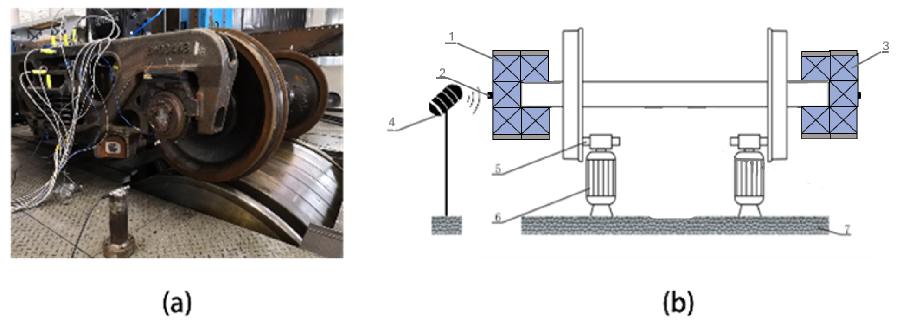
3.1. Experimental Setup and Dataset

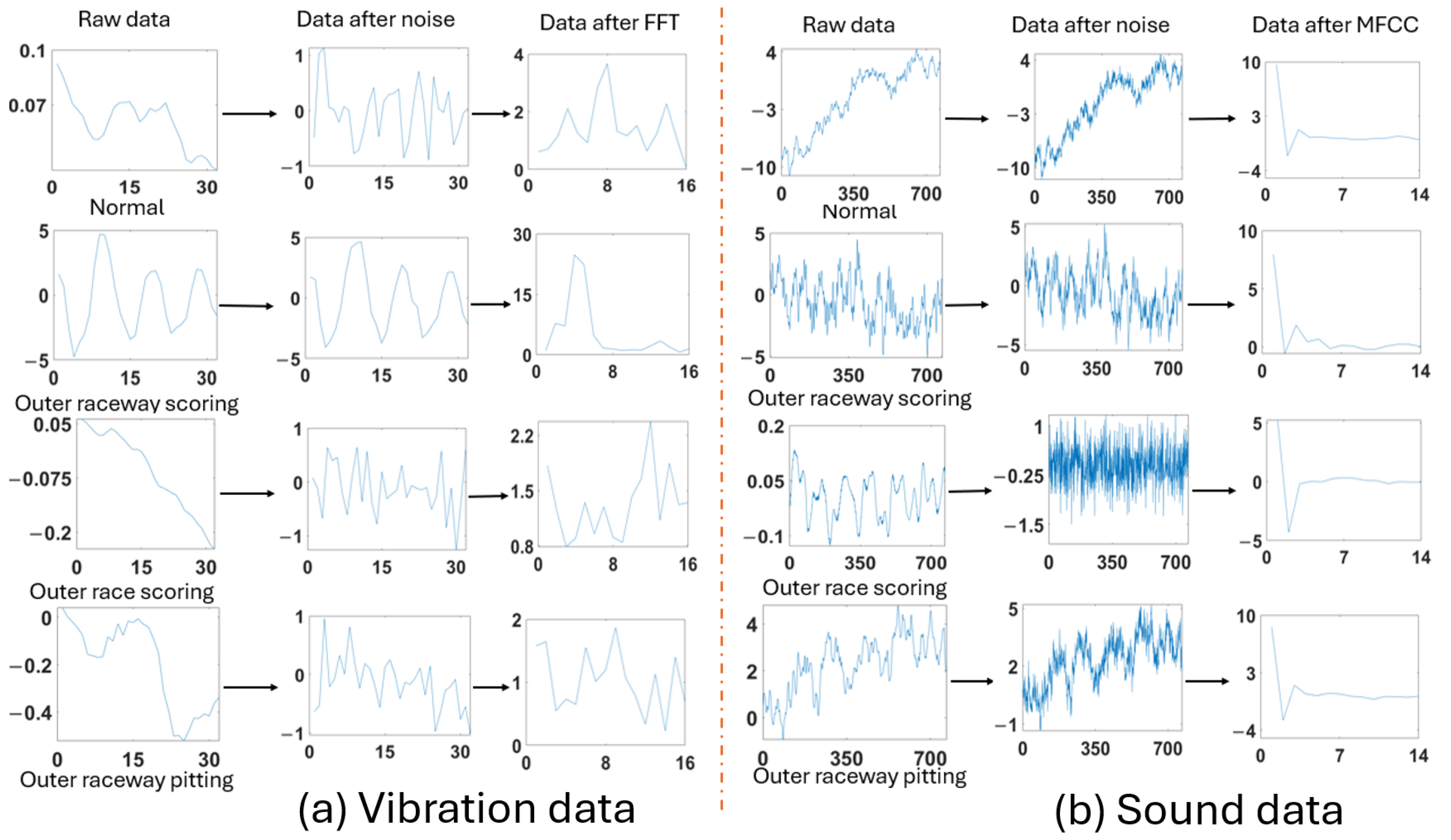
The experiment used MATLAB 2022b and Python 3.9.

This fault detection has high accuracy and fast speed.

There are many sensors on the wheelset bearing. The data used in the experiment were the signal of one of the acceleration sensors and microphone sensors. The data were collected from the bearing in our laboratory. The data were collected at 25,600 samples/second.

Wheelset bearings are essential elements utilized in railway vehicles, including trains, subways, and light rail systems. The axles and wheels are supported by them, carrying the full weight of the vehicle. These bearings need to function consistently and dependably in diverse and intricate circumstances. It is shown in Figure 3a.

In order to monitor the health of bearings, sensors are installed on the bearings. It is shown in Figure 3b which is a cross-sectional view of Figure 3a, among them, 1 is tested bearing, 2 is accelerometer, 3 is auxiliary bearing, 4 is microphone sensor, 5 is friction wheel, 6 is motor, 7 is foundation. The height of the microphone sensor position is 300 mm, and the horizontal distance from the test bearing is 500 mm.

Accelerometers are predominantly employed to capture the vibration signals emitted by bearings. These signals can indicate the operating condition of the bearings, such as the existence of wear, imbalance, misalignment, or other mechanical problems. Microphone sensors are employed to capture the sound emissions generated by bearings during their functioning. Various sorts of flaws produce unique sound characteristics, and by analyzing these sounds, the state of the bearings can be initially evaluated. By integrating accelerometers and microphone sensors, it is possible to monitor and diagnose the operational condition of the bearings in a more comprehensive manner, enabling the quick identification and treatment of potential problems, ensuring the smooth functioning of the equipment.

Four different states are Normal, Outer raceway scoring (referring to damage on the raceway surface where the rolling elements contact), Outer race scoring (a broader term encompassing damage on any part of the outer race), and Outer raceway pitting (refers to the pitting phenomenon on the raceway surface of the outer ring of a bearing). Each state has 1000 segments, each vibration segment has 16 feature samples after FFT, and each sound segment has 14 feature samples after MFCC, concatenating these features to form a single data segment, hence each fusion segment has 30 feature samples.

The data in each state were evenly partitioned into 4 distinct groups with 250 segments each. The validation was performed using a 4-fold cross-validation approach. The details are shown in

Table 2. Dataset was split into training and testing groups for the 4-fold cross-validation.

	Training Group	Testing Group
Validation 1	2, 3, 4	1
Validation 2	1, 3, 4	2
Validation 3	1, 2, 4	3
Validation 4	1, 2, 3	4

.

3.2. Data Analysis

As shown in Figure 4a, the length of each sample of raw vibration data was 32, and then the Gaussian white noise was added to the vibration data. The reason for adding different levels of noise is that the data collected from our laboratory are too clear in comparison with the data from real-world applications. After FFT, the length of each segment is 16. In Figure 4b, the length of each sample of raw sound data was 768 because the default window length in MATLAB depends on the specified sample rate: round (e.g., the number of frequency sampling × 0.03) and the frequency sampling is 25,600 samples/second, and then the Gaussian white noise is added to the sound data. After MFCC, the length of each segment is 14.

As shown in Figure 5, the length of each sample of fusion data was 30, the difference states at the peak value were obvious.

3.3. Experimental Results

In this experiment, ten comparative networks were introduced to validate the performance and confirm the accuracy of each method. To validate the performance of the methodology, the Neural Network and SVM comparison models in MATLAB were introduced.

3.3.1. Comparison Performance

In this part, the fusion data were trained and tested with a few neural network methods and SVM methods [37]. In this section, the fusion data underwent training and testing using several neural network and SVM algorithms [37]. For neural network methods, the best method was the Trilayered Neural Network, whose accuracy was 97.8%. For SVM methods, the best method was the Quadratic SVM, whose accuracy was 97.9%. The accuracy data are shown in Figure 6. Among these 10 methods, the best result was demonstrated by Quadratic SVM. Additionally, the model of SVM is simpler than neural network. This means SVM can achieve superior efficiency in data detection compared to neural networks. Hence, the suggested approach opts for SVM and enhances its performance by incorporating GWO.

3.3.2. Training Loss

For the proposed method, the model output was used to classify tasks (using ‘SVM’). The training loss exhibits a quick decline in the initial iterations and thereafter reaches a stable state in the middle stages. This suggests that the process of training the model has achieved a state of convergence after 200 iterations, as is shown in Figure 7.

4. Discussion

To create a functional model, it is necessary to achieve a high level of accuracy with real-time capability.

4.1. Evaluation of Different Lengths in Each Segment

In this part, five SVM methods in MATLAB are used for different lengths of testing in each segment, including lengths of 256, 128, 64, and 32. The results are shown in

Table 3. Testing accuracy of different lengths in each segment.

SVM Method	Data Types	Length
		256	128	64	32
Linear SVM	Vibration	100%	98%	98%	97%
	Sound	99%	100%	99%	97%
Cubic SVM	Vibration	100%	100%	99%	98%
	Sound	99%	100%	98%	97%
Quadratic SVM	Vibration	100%	100%	98%	98%
	Sound	99%	100%	98%	97%
Coarse Guassian SVM	Vibration	100%	99%	99%	97%
	Sound	99%	100%	97%	93%
Medium Gaussian SVM	Vibration	99%	99%	99%	96%
	Sound	99%	100%	100%	98%

, for the length of 32, the best accuracy achieved is 98% which shows that the length of 32 in each segment contains enough characteristic information.

4.2. Evaluation of Proposed Method Performance

In this part, the GWO-SVM method initializes the number of wolves as n = 10 and the number of iterations as L = 200; The software executes using a 4-fold cross-validation approach, with each group being repeated 5 times. Following each iteration, the wolves undergo a sorting process based on their fitness values, which allows for the identification of the three wolves with the greatest fitness levels. These wolves are referred to as the alpha, beta, and delta wolves. The alpha wolf is prioritized due to its superior fitness. The ultimate trained model exclusively utilizes the parameters of the alpha wolf.

For vibration data and sound data, as shown in

Table 4. Description of different segments.

Kernel of SVM	Training Model	Vibration Accuracy	Sound Accuracy	Fusion Accuracy
Linear SVM	Matlab	67.6%	97.4%	97.8%
	GWO-SVM	68%	97.6%	98.3%
Quadratic SVM	Matlab	67.4%	97.2%	97.9%
	GWO-SVM	67.7%	97.3%	98%
Cubic SVM	Matlab	66.8%	95.5%	97.5%
	GWO-SVM	66.8%	97.2%	97.7%
Gaussian SVM	Matlab-Medium Gaussian SVM	68%	97.6%	97%
	Matlab-Coarse Gaussian SVM	67.9%	95.2%	94.3%
	GWO-SVM	68.1%	97.7%	98.1%

, the best result in Matlab was Medium Gaussian SVM, whose accuracy was 68% in vibration data and 97.6% in sound data, respectively. The result obtained by the GWO-SVM model using Medium Gaussian SVM was 68.1% and 97.7%, respectively.

For fusion data, a comparison was made between the GWO-SVM in Python and the SVM method in MATLAB. As shown in Table 4, the best result in MATLAB was Quadratic SVM, whose accuracy was 97.9%; The result obtained by the GWO-SVM model using Quadratic SVM was 98%. Additionally, the best result in GWO-SVM was Linear GWO-SVM, whose accuracy was 98.3%.

It is obvious from Table 4 that the proposed method had a better performance than the traditional SVM methods in both vibration, sound and fusion data.

4.3. Evaluation of Testing Speed

This experiment measures the total testing time for all 1000 testing segments and then calculates its average for each segment.

In this part, as shown in

Table 5. Test results and time of fusion data.

Different Kernel of GWO-SVM	Accuracy	Testing Time for Each Segment	Sampling Time
Linear SVM	98.3%	0.0027 ms	31.25 ms
Quadratic SVM	98%	0.0034 ms
Cubic SVM	97.7%	0.0035 ms
Gaussian SVM	98.1%	0.016 ms

, the testing time was tested with different SVM kernels in Python: linear kernel, gaussian kernel (rbf kernel) and quadratic-cubic kernel (polynomial kernel). The frequency sampling was 25,600 samples/second, the sampling time for each segment of vibration data was 1.25 ms and the sampling time for each segment of sound data was 30 ms; thus, the sampling time for each segment of fusion data was 31.25 ms.

The proposed method demonstrates high efficiency in processing fusion data, enabling rapid analysis and prediction with a remarkable speed of 0.0027 milliseconds per data segment. The experimental results indicate that the model attains a 98.3% accuracy in promptly recognizing wheelset bearing defects. The proposed method exhibited superior performance in terms of both accuracy and execution time when compared to the comparative model. The proposed method exhibited exceptional performance and is in line with the specified requirements.

It should be mentioned here, this excellent experimental performance is based on this single case only, where there are only three fault and normal situations under our limited equipment conditions. However, it will be straightforward to extend our method to any other scenarios where more fault and sensors can be used in real situations. Of course, more evaluations are needed.

5. Conclusions

This work developed a GWO-SVM model for real-time identification of defects in wheelset bearings. The model was developed and trained using the Python programming language. Subsequently, the model was executed on a desktop computer to replicate fast wheelset bearing fault detection for possible real-time implementation. The results of the experiment show that the model achieves accuracy and quickly identifies faults within milliseconds of their occurrence. It achieved an accuracy rate of 98.3% with a testing duration of 0.0027 ms proving its effectiveness and precision in detecting wheelset bearing defects.

This work demonstrates the practical ramifications as well as potential uses of real-time identification of faults in wheelset bearings using a GWO-SVM model. The model demonstrates remarkable precision in rapidly detecting bearing defects and promptly making forecasts, leading to decreased maintenance expenses, enhanced bearing accessibility, and improved overall effectiveness. By promptly detecting malfunctions during the operation of bearings, this model enables early detection and swift action, thereby reducing downtime and decreasing maintenance expenses.

While this study has made notable progress, there remains a substantial amount of effort to enhance the effectiveness and practicality of the suggested approach. Some guidelines for future endeavors include the following: 1. Enhanced data sources: Subsequent studies can explore the inclusion of other sensor data, such as temperature and pressure, to enhance the comprehensiveness and precision of defect identification. 2. Adaptive Algorithm Optimization: In real-world scenarios, researchers investigate adaptive optimization algorithms that allow the model to autonomously modify parameters according to the environment and operating conditions, thereby improving the model’s resilience. 3. Long-term Performance Evaluation: Conduct long-term performance evaluations and maintenance cost analyses to verify the economic benefits and sustainability of the proposed method in practical operations. By exploring and improving these future work directions, it is expected that the performance and application of the GWO-SVM method in bearing fault detection can be further enhanced, providing a more reliable and efficient industrial maintenance solution.

References

1. Yadav, O.P.; Pahuja, G.L. Bearing health assessment using time domain analysis of vibration signal. Int. J. Image Graph. Signal Process. 2020, 10, 27. [Google Scholar] [CrossRef]
2. NCD.IO. Bearing Fault Detection Vibration Analysis-How to Measure Vibration Frequency Domain Predictive Analysis. Available online: https://ncd.io/blog/bearing-fault-detection-vibration-analysis/ (accessed on 23 June 2023).
3. Altaf, M.; Akram, T.; Khan, M.A.; Iqbal, M.; Ch, M.M.I.; Hsu, C.H. A new statistical features based approach for bearing fault diagnosis using vibration signals. Sensors 2022, 22, 2012. [Google Scholar] [CrossRef]
4. Kumar, J.P.; Chauhan, P.S.; Pandit, P.P. Time domain vibration analysis techniques for condition monitoring of rolling element bearing: A review. Mater. Today Proc. 2022, 62, 6336–6340. [Google Scholar] [CrossRef]
5. Wang, T.; Qin, R.; Meng, H.; Li, M.; Cheng, M.; Liu, Y. Frequency Domain Feature Extraction and Long Short-Term Memory for Rolling Bearing Fault Diagnosis. In Proceedings of the 2022 International Conference on Machine Learning, Control, and Robotics (MLCR), Suzhou, China, 29–31 October 2022. [Google Scholar]
6. Chen, B.; Gu, F.; Zhang, W.; Song, D.; Cheng, Y.; Zhou, Z. Power function-based Gini indices: New sparsity measures using power function-based quasi-arithmetic means for bearing condition monitoring. Struct. Health Monit. 2022, 22, 3677–3706. [Google Scholar] [CrossRef]
7. Huang, P.; Pan, Z.; Qi, X.; Lei, J. Bearing fault diagnosis based on EMD and PSD. In Proceedings of the 2010 8th World Congress on Intelligent Control and Automation, Jinan, China, 7–9 July 2010; pp. 1300–1304. [Google Scholar]
8. Chen, B.; Zhang, W.; Song, D.; Cheng, Y.; Gu, F.; Ball, A.D. Squared envelope sparsification via blind deconvolution and its application to railway axle bearing diagnostics. Struct. Health Monit. 2023, 22, 3637–3658. [Google Scholar] [CrossRef]
9. Baba, T. Time-frequency analysis using short time Fourier transform. Open Acoust. J. 2012, 5, 32–38. [Google Scholar] [CrossRef]
10. Zhang, D. Wavelet transform. In Fundamentals of Image Data Mining: Analysis, Features, Classification and Retrieval; Springer: Cham, Switerland, 2019; pp. 35–44. [Google Scholar]
11. Yu, G. A concentrated time–frequency analysis tool for bearing fault diagnosis. IEEE Trans. Instrum. Meas. 2019, 69, 371–381. [Google Scholar] [CrossRef]
12. Zhang, Q.; Yang, J.; An, Q. Noise calculation method for deep groove ball bearing with considering raceway surface waviness and roller size error. Front. Mech. Eng. 2018, 4, 13. [Google Scholar] [CrossRef]
13. BearingNews. Diagnosing Bearing Failures Using Ultrasound Spectrum Analysis. 2022. Available online: https://www.bearing-news.com/diagnosing-bearing-failures-using-ultrasound-spectrum-analysis/ (accessed on 26 April 2022).
14. Heckbert, P. Fourier transforms and the fast Fourier transform (FFT) algorithm. Comput. Graph. 1995, 2, 15–463. [Google Scholar]
15. Huang, N.E.; Shen, Z.; Long, S.R.; Wu, M.C.; Shih, H.H.; Zheng, Q.; Yen, N.C.; Tung, C.C.; Liu, H.H. The empirical mode decomposition and the Hilbert spectrum for nonlinear and non-stationary time series analysis. Proc. R. Soc. London. Ser. A Math. Phys. Eng. Sci. 1998, 454, 903–995. [Google Scholar] [CrossRef]
16. Hiremath, N.; Reddy, D.M. Bearing fault detection using acoustic emission signals analyzed by empirical mode decomposition. Int. J. Res. Eng. Technol. 2014, 3, 426–431. [Google Scholar]
17. Grebenik, J.; Zhang, Y.; Bingham, C.; Srivastava, S. Roller element bearing acoustic fault detection using smartphone and consumer microphones comparing with vibration techniques. In Proceedings of the 2016 17th International Conference on Mechatronics-Mechatronika (ME), Prague, Czech Republic, 7–9 December 2016; pp. 1–7. [Google Scholar]
18. Li, C.; Chen, C.; Gu, X. Acoustic-Based Rolling Bearing Fault Diagnosis Using a Co-Prime Circular Microphone Array. Sensors 2023, 23, 3050. [Google Scholar] [CrossRef]
19. Orman, M.; Rzeszucinski, P.; Tkaczyk, A.; Krishnamoorthi, K.; Pinto, C.T.; Sulowicz, M. Bearing fault detection with the use of acoustic signals recorded by a hand-held mobile phone. In Proceedings of the 2015 International Conference on Condition Assessment Techniques in Electrical Systems (CATCON), Bangalore, India, 10–12 December 2015; pp. 252–256. [Google Scholar]
20. Attal, E.; Asseko, E.O.; Sekko, E.; Sbai, N.; Ravier, P. Study of bearing fault detectability on a rotating machine by vibro-acoustic characterisation as a function of a noisy surrounding machine. In Surveillance, Vibrations, Shock and Noise; Institut Supérieur de l’Aéronautique et de l’Espace: Toulouse, France, 2023. [Google Scholar]
21. Mey, O.; Schneider, A.; Enge-Rosenblatt, O.; Mayer, D.; Schmidt, C.; Klein, S.; Herrmann, H.-G. Condition Monitoring of Drive Trains by Data Fusion of Acoustic Emission and Vibration Sensors. Processes 2021, 9, 1108. [Google Scholar] [CrossRef]
22. Kaicheng, Y.; Chaosheng, Z. Vibration data fusion algorithm of auxiliaries in power plants based on wireless sensor networks. In Proceedings of the 2011 International Conference on Computer Science and Service System (CSSS), Nanjing, China, 27–29 June 2011; pp. 935–938. [Google Scholar]
23. Xuejun, L.; Guangfu, B.; Dhillon, B.S. A new method of multi-sensor vibration signals data fusion based on correlation function. In Proceedings of the 2009 WRI World Congress on Computer Science and Information Engineering, Los Angeles, CA, USA, 31 March–2 April 2009; Voulme 6, pp. 170–174. [Google Scholar]
24. Al-Haddad, L.A.; Jaber, A.A.; Hamzah, M.N.; Fayad, M.A. Vibration-current data fusion and gradient boosting classifier for enhanced stator fault diagnosis in three-phase permanent magnet synchronous motors. Electr. Eng. 2024, 106, 3253–3268. [Google Scholar] [CrossRef]
25. Wan, H.; Gu, X.; Yang, S.; Fu, Y. A Sound and Vibration Fusion Method for Fault Diagnosis of Rolling Bearings under Speed-Varying Conditions. Sensors 2023, 23, 3130. [Google Scholar] [CrossRef] [PubMed]
26. Shi, H.; Li, Y.; Bai, X.; Zhang, K.; Sun, X. A two-stage sound-vibration signal fusion method for weak fault detection in rolling bearing systems. Mech. Syst. Signal Process. 2022, 172, 109012. [Google Scholar] [CrossRef]
27. Duan, Z.; Wu, T.; Guo, S.; Shao, T.; Malekian, R.; Li, Z. Development and trend of condition monitoring and fault diagnosis of multi-sensors information fusion for rolling bearings: A review. Int. J. Adv. Manuf. Technol. 2018, 96, 803–819. [Google Scholar] [CrossRef]
28. Wang, X.; Mao, D.; Li, X. Bearing fault diagnosis based on vibro-acoustic data fusion and 1D-CNN network. Measurement 2021, 173, 108518. [Google Scholar] [CrossRef]
29. Gu, X.; Tian, Y.; Li, C.; Wei, Y.; Li, D. Improved SE-ResNet Acoustic–Vibration Fusion for Rolling Bearing Composite Fault Diagnosis. Appl. Sci. 2024, 14, 2182. [Google Scholar] [CrossRef]
30. Mirjalili, S.; Mirjalili, S.M.; Lewis, A. Grey wolf optimizer. Adv. Eng. Softw. 2014, 69, 46–61. [Google Scholar] [CrossRef]
31. Hearst, M.A.; Dumais, S.T.; Osuna, E.; Scholkopf, B. Support vector machines. IEEE Intell. Syst. Their Appl. 1998, 13, 18–28. [Google Scholar] [CrossRef]
32. Yan, X.; Lin, Z.; Lin, Z.; Vucetic, B. A Novel Exploitative and Explorative GWO-SVM Algorithm for Smart Emotion Recognition. IEEE Internet Things J. 2023, 10, 9999–10011. [Google Scholar] [CrossRef]
33. Davis, S.; Mermelstein, P. Comparison of parametric representations for monosyllabic word recognition in continuously spoken sentences. IEEE Trans. Acoust. Speech Signal Process. 1980, 28, 357–366. [Google Scholar] [CrossRef]
34. Pule, M.; Matsebe, O.; Samikannu, R. Application of PCA and SVM in fault detection and diagnosis of bearings with varying speed. Math. Probl. Eng. 2022, 2022, 5266054. [Google Scholar] [CrossRef]
35. Yang, K.; Zhao, L.; Wang, C. A new intelligent bearing fault diagnosis model based on triplet network and SVM. Sci. Rep. 2022, 12, 5234. [Google Scholar] [CrossRef] [PubMed]
36. Mo, C.; Han, H.; Liu, M.; Zhang, Q.; Yang, T.; Zhang, F. Research on SVM-Based Bearing Fault Diagnosis Modeling and Multiple Swarm Genetic Algorithm Parameter Identification Method. Mathematics 2023, 11, 2864. [Google Scholar] [CrossRef]
37. Selvi, M.S.; Rani, S.J. Classification of admission data using classification learner toolbox. J. Phys. Conf. Ser. 2021, 1979, 12043. [Google Scholar] [CrossRef]
Figure 1. Overview of the system: (a) wheelset; (b) modeling in python language; (c) GWO-SVM model; and (d) predictions.
Technologies 12 00144 g001
Figure 2. Proposed model.
Technologies 12 00144 g002
Figure 3. Data collection platform. (a) Wheelset bearings; (b) sensor installation location.
Technologies 12 00144 g003
Figure 4. Data spectrum. (a) vibration data; (b) sound data.
Technologies 12 00144 g004
Figure 5. Fusion data.
Technologies 12 00144 g005
Figure 6. Comparison of accuracy of fusion data in Matlab classification learner.
Technologies 12 00144 g006
Figure 7. The loss curve of changes with training progress.
Technologies 12 00144 g007