Abstract
In this paper, the dataset is collected from the fluidic muscle datasheet. This dataset is then used to train models predicting the pressure, force, and contraction length of the fluidic muscle, as three separate outputs. This modeling is performed with four algorithms—extreme gradient boosted trees (XGB), ElasticNet (ENet), support vector regressor (SVR), and multilayer perceptron (MLP) artificial neural network. Each of the four models of fluidic muscles (5-100N, 10-100N, 20-200N, 40-400N) is modeled separately: First, for a later comparison. Then, the combined dataset consisting of data from all the listed datasets is used for training. The results show that it is possible to achieve quality regression performance with the listed algorithms, especially with the general model, which performs better than individual models. Still, room for improvement exists, due to the high variance of the results across validation sets, possibly caused by non-normal data distributions.
1. Introduction
Fluidic muscles, also sometimes referred to as pneumatic or hydraulic muscles, are devices that mimic the function of biological muscles using air or liquid as a force transmission medium. Pneumatic muscles use compressed air as the working fluid, expanding when air is introduced into the muscle, generating force. Hydraulic muscles work in the same manner, with the air being replaced by a liquid—usually hydraulic oil. Fluidic muscles are commonly applied in robotics to create biological movements in robotic systems, with smoother and more flexible motion compared to classic actuators [1]. Due to their high force output and possibility for precise control, fluidic muscles are sometimes used in industrial applications [2]. Finally, fluidic muscles are often used in biomechanics—especially for rehabilitation and the creation of prosthetics [3].
Using soft actuators like fluidic muscles requires highly accurate models to predict their behavior. Antonson (2023) [4] compared two modeling techniques, Maxwell-slip and Bouc–Wen, for predicting muscle force, reporting normalized mean absolute percentage errors of 5.37% and 12.84%, respectively. Garbulinski et al. (2021) [5] employed several models—including linear, polynomial, exponential decay, and exponent—to predict fluidic muscle strain. The respective errors for these models were 4.12% (linear), 2.10% (polynomial), 1.94% (exponential decay), and 1.92% (exponent). Trojanova et al. (2022) [6] assessed parsimonious machine learning models for static fluidic muscle modeling. The best models, based on MLP, had errors ranging from 10.10% to 1.26%, though each muscle was modeled individually.
The papers show that, while the authors have performed the modeling of individual muscles in the previous research, two shortcomings can be identified as knowledge gaps. First, the authors model different variations of fluidic muscles separately. This means that a generalized model is not achieved. In an industry application, this means that the engineer would need to select an appropriate model from the library, which can lead to errors. Second, authors tend to focus on actuation force modeling, which is only one of the three main physical quantities that describe the behavior of fluidic muscles; so, models that can be used in situations where the force is known are not explored.
A highly precise model that can be applied regardless of fluidic muscle dimensions (i.e., one that is developed generally, not for a specific dimension/model of the actuator) can have wide applications. As noted by Hamon et al. [7], such muscles can be used as the main actuating components of robotic grippers. Having rapid controller software that determines the necessary pressure for the given desired force and contraction percentage would allow for a simpler implementation and the possibility of using a single controller algorithm for multiple dimensions of grippers, greatly simplifying the production and implementation of such end-effectors. Pietrala et al. [8] demonstrated the possibility of usage of fluidic muscles as actuators in a 6-DOF parallel manipulator. They proposed a complex mathematical model for determining the pressure of a muscle necessary to achieve a given position and force. Not only could this potentially be simplified with the application of machine learning but it would also simplify the possibility of using fluidic muscles as actuators in serial robotic manipulators, where different dimensions, contraction lengths, and forces may be necessary to achieve a desired configuration. Outside of industrial applications, Tsai and Chiang [9] demonstrated the applications of fluidic muscles for the rehabilitation of lower limbs. With differing lengths of limbs in patients, a more general model that will allow a precise determination of the pressure necessary can simplify the applications of such techniques in rehabilitation. Another possible application of such generalized and high-precision models is wearable tech, as commented by Wang et al. [10]. Small high-contraction fluidic muscles can benefit from a more general application by having a single controller for various, differently sized, actuators, allowing for simpler implementation. The final notable application of fluidic muscles that can benefit from a general high-precision model with quick calculation times that could be obtainable from ML algorithms is the antagonistic arrangement, such as noted by Tuleja et al. [11], in which multiple muscles of different sizes are working at the same time in order to achieve a certain configuration. Again, using a single algorithm to control all of the muscles involved in this antagonistic arrangement could simplify the control procedure.
The goal of this paper is to test the modeling performance that targets the single model of a fluidic muscle and compare it to a model that includes data points of multiple variations of fluidic muscles. The goal of this is to test the possibility of creating a more general model of a fluidic muscle.
The authors first generate a dataset from the manufacturer-provided datasheets. Then, these datasets are analyzed and compared. The authors then create a set of models that aim at modeling three separate outputs—the actuation force, contraction, and pressure. Actuation force is the force that is exhibited by fluidic muscle when pressure is applied to it. Contraction represents the percentage by which the length of the muscle is shortened when the pressure is applied during actuation. Finally, pressure represents the amount of pressure necessary to achieve the actuation force at a given contraction [12].
2. Methodology
This section will describe how the dataset was obtained and combined into a complete dataset. Then, ML-based regression techniques used will be described, along with the evaluation process.
2.1. Obtaining the Dataset
The dataset was obtained from the DMSP fluidic muscle datasheet [12]. In the document, parameters are provided for four separate variations of fluidic muscles:
- DMSP-5-100N;
- DMSP-10-100N;
- DMSP-20-200N;
- DSMP-40-400N.
For each of the above fluidic muscle variations, the following parameters are noted:
- Diameter;
- Minimal nominal length;
- Maximal nominal length;
- Maximal stroke;
- Maximal additional load;
- Maximal pre-tensioning;
- Maximal contraction.
In addition to the above, each of the muscles is provided with a chart displaying a contraction h [%] on the x-axis, with force F [N] on the y-axis, for different pressure values p [bar]. These diagrams are scanned using WebPlotDigitizer software, which allows them to be converted to a numerical dataset. These values can be plotted and are shown in Figure 1. The presented figures are visually inspected to confirm that they match the source data well, and the values can be used in further analyses.
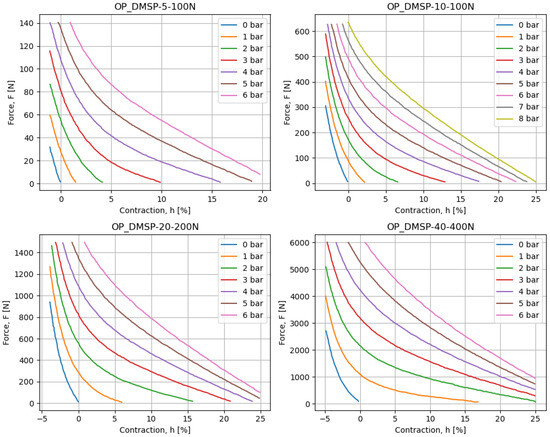
Figure 1.
The data charts for different fluidic muscles, as collected based on the figures provided in the datasheet.
The previously listed values for each of the fluidic muscles are noted and combined with the previously mentioned data (e.g., diameter) in a table in such a way that each of the metrics is given as a column. While this process results in constant columns in the individual datasets, these values will allow for further differentiation of the data when the datasets are combined. The above process results in four datasets, with data points in each dataset given in Table 1.

Table 1.
The amount of data in each of the obtained datasets for separate fluidic muscles.
The differing amount of the points in the dataset stems from the WebPlotDigitizer methodology and the fact that not all dataset images which were used for data collection using the aforementioned software had the same amount of data lines present. While the difference in data points can have some influence on the models and scores, all the datasets have a large enough amount of data points, enabling them to not adversely affect models. In other words, all datasets are large enough to train the models. The datasets are combined by stacking them and shuffling them in preparation for later AI training. This results in the final dataset, which consists of 5452 data points. Following this, the correlation of columns in the final dataset is measured to determine whether they influence the outputs or not. Additionally, each dataset has its main descriptive statistics (mode, mean, min, max, standard deviation, skewness, and kurtosis) analyzed for F and h values (p was skipped due to the values being discrete and limited), to compare them to the final dataset. Finally, histograms are calculated for the collected and combined datasets to compare the distributions.
2.2. Regression Techniques Applied
The manuscript applies four algorithms—multilayer perceptron (MLP), support vector regressor (SVR), ElasticNet (ENet), and extreme gradient boosted machines (XGB). MLP was selected due to its known good performance in various tasks. The algorithms in question were selected due to their known good performance on similar tasks—with MLP being known to provide extremely precise models when a large amount of data are available. In turn, SVR bases itself on the key points in data to create the model, hence eliminating the influence of larger data amounts in certain ranges of data (a possible concern, as will be shown later in this paper), with ENet being selected for a similar reason and its good expected performance on the linear data. Finally, XGB was selected both due to its good performance but also for its ability to provide a set of interpretable tree-shaped models, which may be easier to implement in comparison to models resulting from other algorithms.
The overview of the methodology is given as follows, with a more detailed descriptions given in the continuation of this paper:
- The dataset is selected by selecting the following:
- (a)
- The dataset for a single fluidic muscle or the combined dataset;
- (b)
- The target value between force, pressure, and contraction (with the remaining two used as outputs).
- The selected dataset is split into five parts for a cross-validation procedure.
- The loop is repeated as follows:
- (a)
- Out of all possible given hyperparameter combinations, one is selected;
- (b)
- A dataset fold is formed using four parts as a training set and one as a testing set;
- (c)
- The training set is split into training/validation and the model is created;
- (d)
- The trained model is evaluated on the testing set with two metrics.
- After the previous steps are completed, the fold is evaluated, and the mean scores and standard deviations are noted.
- The best model hyperparameters are selected based on those scores.
This procedure is repeated for each of the datasets used in this study. The results are presented in Section 3.
2.2.1. Evaluation and Training Procedure
Each of the regression techniques is applied in the same methodological manner. Each dataset is randomly divided into five parts. The model is then trained on a combination of four parts, while the remaining part is used to test the model’s performance. This process is repeated five times, using a different subset as the test set for each iteration. This method, called k-fold cross-validation, uses in this example [13,14]. Each subset combination is referred to as a fold. In addition to this, grid search tuning is used for hyperparameter tuning. In this process, a set of discrete values for each of the method hyperparameters is set. Then, the aforementioned k-fold cross-validation is performed for each possible set of hyperparameter combinations [15,16]. The scores are calculated for each training fold—as the average between the five values and the standard deviation of that set of values—and each hyperparameter combination. Models are evaluated using the coefficient of determination () [17], which defines the amount of variance in the original data explained in the predictions, denoted as
where is the real value contained in the dataset, and is the predicted value obtained from the model. A higher value for produces a better result, in the range of . While the serves as a good predictor, it can incorrectly validate scores in some cases due to it taking only variation into account. Because of this, another metric is applied to determine the absolute error of the model across predictions. The metric used is the mean absolute percentage error, . This metric was selected because it allows for an easier comparison of models across different targets since they are not the same physical quantity. is defined as
2.2.2. Multilayer Perceptron
MLP is a feedforward artificial neural network consisting of neurons arranged into hidden layers. Each of the neurons in one layer is connected to all of the neurons in the subsequent layer, via a weighted connection. In each neuron, an operation is performed that multiplies the value of each of the neurons in the previous layer with the weights of appropriate connections and sums them, passing them through an activation function, which controls the output [18]. By introducing the values of input variables to the input neurons and performing the weighted summation, the value of the single neuron in the final layer and the output of the neural network are calculated. Then, for the predicted value , the error is calculated in comparison to the real value y. Then, the weights of the neuron connections are adjusted based on the gradient of this error [19].
Apart from the weights, which are the network’s parameters, hyperparameters also significantly affect performance. These hyperparameters comprise the number of layers and neurons, as well as the activation functions that were mentioned previously. However, in addition to that, there are others—such as the algorithm used for the adjustment of connection weights (solver), the initial learning rate and the type of the learning rate that control how quickly is the weight adjusted, and L2 regularization, which controls the influence of higher-influencing variables in the dataset [20].
These values have an extremely high influence on performance [21], and while the initial tuning can be performed based on experience, these values need to be tuned more precisely. The process that is used by the researchers in this paper for this, as well as for the methods that will be described subsequently, is the so-called grid search (GS) method. In this method, the possible values of each hyperparameter are defined as a vector of discrete values. Then, each combination of these values is used to train the network, and performance is tested to evaluate how well a certain combination performs [22]. This method is computationally intensive, but it leads to a relatively precise determination of well-performing hyperparameters. The possible values for selected hyperparameters are given in Table 2.
Table 2.
The possible hyperparameters of the MLP method tested in the GS.
2.2.3. Support Vector Regressor
Support vector regressor (SVR) regression is a supervised machine learning algorithm used for predicting continuous outcomes. Unlike the multilayer perceptron (MLP), SVR regression does not involve a complex network of interconnected neurons. Instead, it focuses on identifying a hyperplane that best fits the data points while minimizing the error. In SVR regression, the objective is to find the hyperplane with the maximum margin that separates the data points while accommodating some level of error. This margin represents the distance between the hyperplane and the nearest data points, ensuring a robust model [23].
To achieve this, SVR regression employs a set of support vectors, which are data points crucial for determining the hyperplane. These support vectors contribute to the formation of the margin, and their influence is prioritized during the regression process. The algorithm aims to minimize the error between the predicted values and the actual values, allowing for some deviation within the specified error range [24].
Like the MLP, the SVR also has hyperparameters that dictate its behavior and, in turn, performance. They consist of the kernel, which defines the mathematical transformation applied to input features; degree, which is the polynomial degree of the polynomial kernel; gamma, which defines the shape of the decision boundary; and C, which is the value that controls the amount of regularization applied [22]. The possible hyperparameters are given in Table 3.
Table 3.
The possible hyperparameters of the SVR method tested in the GS.
2.2.4. Extreme Gradient Boosted Machines
XGB is a gradient boosting algorithm widely used for supervised learning tasks, particularly regression and classification. Unlike traditional neural network approaches, XGB relies on an ensemble of decision trees to make predictions [25]. In XGB regression, the algorithm sequentially builds a series of decision trees, with each tree attempting to correct the errors of the previous ones. These decision trees are shallow and are often referred to as weak learners. The overall prediction is the sum of predictions from all the trees, weighted by their contribution. Boosting in XGB is a sequential ensemble learning technique that combines the predictive power of multiple weak learners, typically shallow decision trees, to create a robust and accurate predictive model. The boosting process involves iteratively adding new trees to the ensemble, with each subsequent tree trained to correct the errors of the combined predictions of the existing trees. The algorithm assigns weights to training instances, focusing on those that were mispredicted in previous iterations [26].
Hyperparameters tuned in this method are the number of weak estimators and the learning rate. Each of the trees also has a maximum depth and a minimal weight for splitting, defined as a hyperparameter, along with both L1 and L2 regularization parameters [27]. As before, the possible values are shown in Table 4.
Table 4.
The possible hyperparameters of the XGB method tested in the GS.
2.2.5. ElasticNET
ElasticNet is a regression algorithm that merges L1 and L2 regularization to improve model robustness and feature selection. Unlike some other regression methods, ElasticNet simultaneously applies both Lasso (L1) and Ridge (L2) penalties to the linear regression cost function. The combination of these penalties introduces a hyperparameter, alpha, which controls the mix between L1 and L2 regularization [28]. A higher alpha emphasizes Lasso regularization, encouraging sparsity in the model by driving some feature coefficients to exactly zero. This inherent feature selection capability makes ElasticNet particularly useful when dealing with datasets with a large number of features, as it can automatically identify and retain the most relevant ones. By striking a balance between the advantages of L1 and L2 regularization, ElasticNet provides a flexible approach to regression, effectively handling multicollinearity and improving the model’s performance on diverse datasets [29].
The hyperparameters of this method are the alpha value mentioned above, the ratio L1 compared to the regularization L2, the intercept estimation, and the algorithm for the selection of random values [22]. The possible values are given in Table 5.
Table 5.
The possible hyperparameters of the ENet method tested in the GS.
3. Results and Discussion
This section will present the results of our research, starting with the results of the statistical analysis of the dataset, followed by the results of the regression.
3.1. Dataset Analysis
The descriptive statistics shown in Table 6 show great variance between the datasets for individual fluidic muscles. This indicates non-transferability between models. As expected, the dataset where all data are combined tends to be the average of other values in the dataset, indicating that such a dataset may have a chance of predicting the values from all datasets; in other words, it is not skewed too greatly to either of the sets. It should be noted that pressure, as the output, was not used in some of the presented statistical analyses due to it only having a few possible discrete values, instead of it being a continuous variable.
Table 6.
The descriptive statistics of the datasets.
By observing the correlation table given in Figure 2, we can see that there is not a high correlation between any of the targeted output values. Correlations are especially low for the pressure output, looking at all possible inputs that may be extracted from the available data. This is possibly due to the discrete nature of the pressure collected from the datasheet.
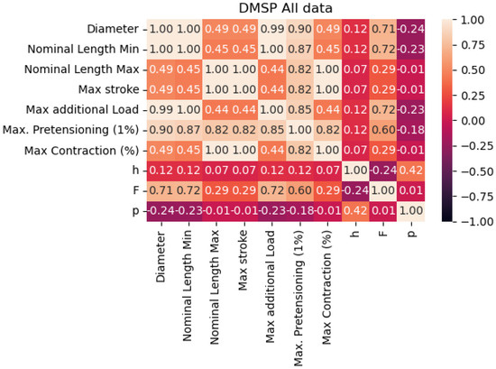
Figure 2.
Correlation of the data points in the combined dataset.
The dataset distributions are important to note. Even with the large amount of data, skewness of the data from the normal distribution could indicate possible issues with the resulting models, and, as such, would warrant a cross-validation scheme. This skewness, towards the start of the dataset, is shown for all datasets in Figure 3, showing that most of the data are given for shorter changes in length, which is apparent in all of the datasets, including the combined dataset.
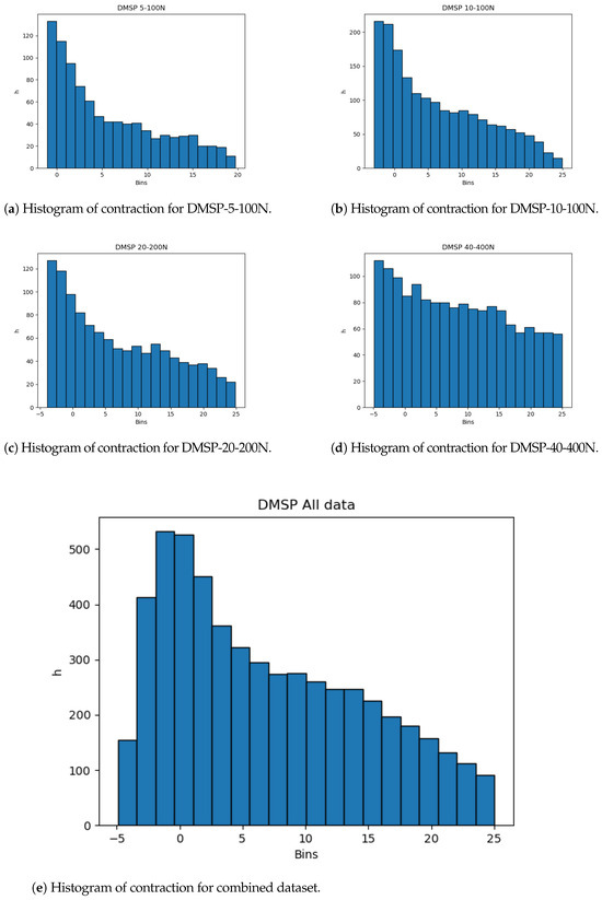
Figure 3.
Histograms of contraction output.
The same is apparent in the datasets for force, as given in Figure 4. While the individual datasets here are less drastic in skewness, the combined dataset practically follows an exponential distribution, with a vast majority of data points being present in the lower end of the data range. Due to this, the use of cross-validation is key to guarantee that the entirety of the dataset is tested.
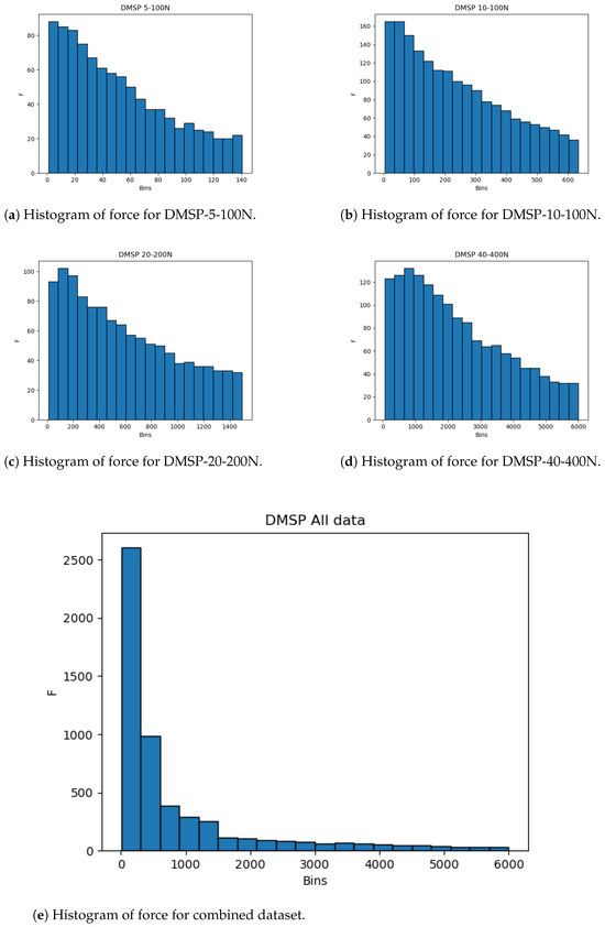
Figure 4.
Histograms of force outputs.
The histograms show that more data are present in the lower end of the data range. While this is less expressed for contraction, it is very apparent for the combined force dataset (Figure 4). This may adversely affect the precision of the created models at the higher end of the data range due to the lower amount of data, and it is safe to assume that most errors will result from this part of data being predicted.
3.2. Regression Results
The complete regression results, for all methods, fluidic muscles, and targets are given in Table 7. The results are given as a mean across the training folds for both and , as well as —the standard error across folds in both cases. The rows are split by the target—force, pressure, or length (contraction)—and are then further split per each of the available models of fluidic muscles: 5-100N, 10-100N, 20-200N, and 40-400N. With the overview of the table, we can conclude that some of the models achieved satisfactory results. For an easier look into the data, the results are presented as figures for each of the fluidic muscles individually later in this manuscript. Overall, the results for pressure seem to be lower than either of the two other outputs, possibly due to the discrete nature of the data.
Table 7.
The results of all applied regression models to all targets.
For the DMSP-5-100N fluidic muscle, we present its results in Figure 5. In the case of contraction models, the best results were achieved by the SVR, at . Still, this model exhibited a large of 4.47%. Significantly smaller was shown by the MLP, but with a much lower —demonstrating the need for multiple metrics. In the case of pressure models, the MLP model achieved the highest of 0.85, with the lowest of 0.01. The SVR achieved a similar , but a significantly higher . Finally, the best results regarding force were obtained with the ENet and MLP models, achieving an of 0.86, with the MLP achieving a significantly lower —0.15% versus 1.16%.
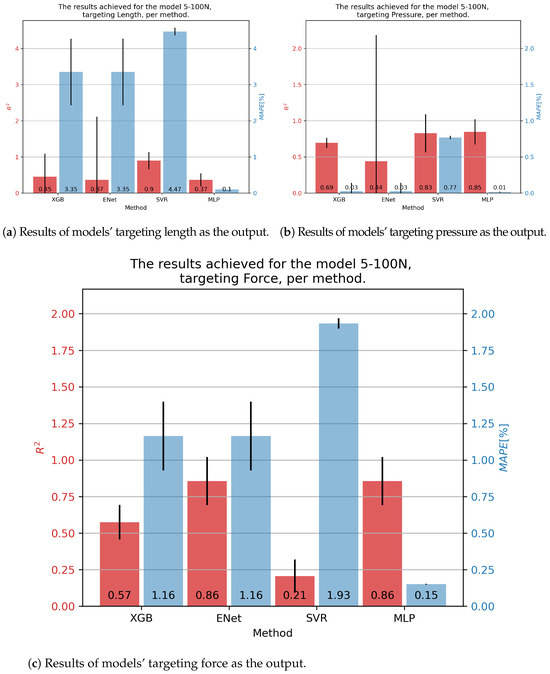
Figure 5.
Best achieved results for DMSP-5-100N. Blue colored bars represent the MAPE, and red represent the score.
In the case of 10-100N fluidic muscle, the pressure was regressed with of 0.92 and of 0.14% using the MLP. Contraction showed much poorer results, with scores indicating that the models barely converged. Interestingly, the errors were low, a phenomenon possibly caused by the models outputting a low-variance output (possibly constant), which was close to the average value of the output that had a comparatively small range. This again indicates the need for multiple metrics being applied, since none of these models can be used for the prediction of values. Force output is somewhat better, with values being approximately 0.80, with the lowest of 0.2 being achieved for the MLP. These results are presented in Figure 6.
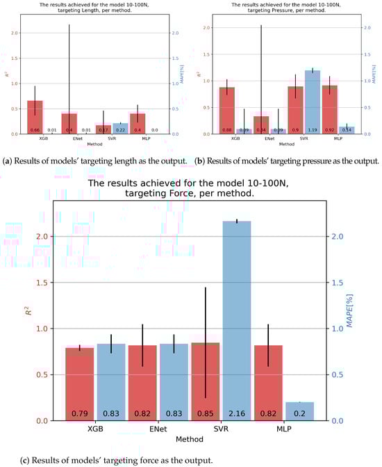
Figure 6.
Best achieved results for DMSP-10-100N. Blue colored bars represent the MAPE, and red represent the score.
In the case of 20-200N fluidic muscle, the results are given in Figure 7. The only model that achieved somewhat good results for contraction was using the SVR—with an of 0.84 and a of 0.80%. Good results ere achieved for pressure with the XGB, SVR, and MLP models, achieving an of approximately 0.92, with the MLP having the lowest of 0.14%. Same behavior was seen regarding force, with the MLP obtaining an of 0.85 and a of 0.17.
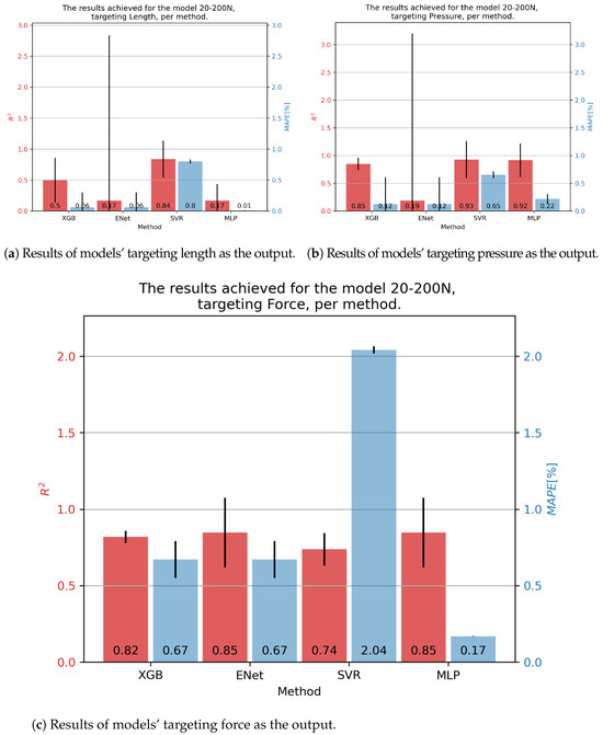
Figure 7.
Best achieved results for DMSP-20-200N. Blue colored bars represent the MAPE, and red represent the score.
Results for the 40-400N muscle are shown in Figure 8. In the case of contraction, the SVR showed the best results, with an of 0.93 and a slightly below 1%. Similar results for pressure were obtained as before, with the MLP achieving the best results with an and a of 0.1%. Force was best predicted with the SVR, but taking into account a high variance in this model’s results, the MLP model was overall a better solution, with an of 0.84 and a of 0.1%.
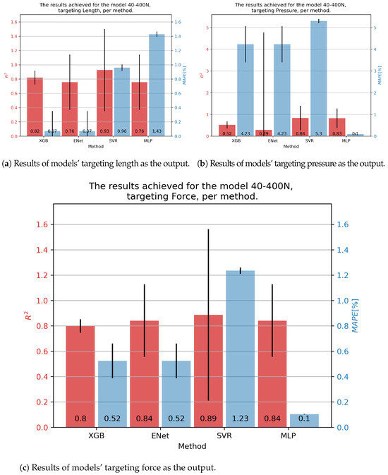
Figure 8.
Best achieved results for DMSP-40-400N. Blue colored bars represent the MAPE, and red represent the score.
We finally arrived at the final results of the manuscript. Figure 9 demonstrates the results achieved on the combined dataset, which was the main goal of this study—testing the possibility of creating a generalized model of fluidic muscles. In order, starting with the contraction percentage, as shown in Figure 9a, the overall best results were achieved with the XGB algorithm, which achieved an score of 0.9 and a of 0.00%. XGB was also the best performing algorithm in both metrics, achieving a mean of 0.92 and a of 0.10% for pressure. For force, the best general prediction was achieved with the MLP, with an of 0.91 and a of 1.46%.
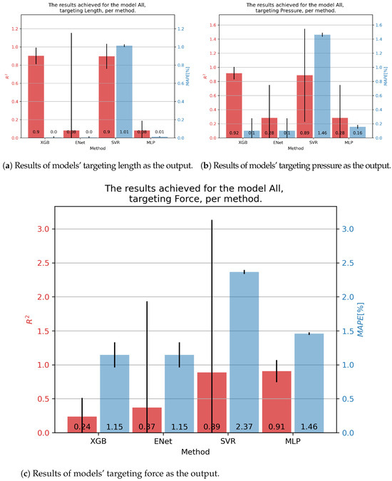
Figure 9.
Best achieved results for DMSP-40-400N. Blue colored bars represent the MAPE, and red represent the score.
The improved results in the combined dataset were possibly caused by the introduction of new variables, which would have been constants in the individual datasets. As shown in the correlation table (Figure 2, these values do have a certain correlation with outputs, indicating that they may be responsible for improved scores, especially with the models based on XGB.
4. Conclusions
This paper aimed to create a generalized model of fluidic muscles, targeting pressure, contraction length, and generated force as targets. These models were created using four algorithms and were compared to the algorithms based on the data of individual fluidic muscles.
The results demonstrate that the general model can be achieved for all three values, and it can have better performance than some of the individual models, possibly due to new information being introduced into the variable space as the dataset was constructed. The overall best results for the combined dataset, regarding the fluidic muscles in general (i.e., the fluidic muscles used in the dataset) were achieved with the XGB algorithm for contraction and pressure, achieving a mean of 0.90 and 0.92, respectively. The best results for force prediction were achieved with the MLP, with an score of 0.91.
However, the model scores show room for improvement due to the relatively high variability of scores across data folds. This issue is probably due to the distribution of the data, with most of the data focused on the lower end of the range. With this research demonstrating the possibility of achieving these results, future work should focus on improving them. Possible applications of synthetic data generation techniques could serve to smooth out probability density functions of data and allow for more robust models.
Author Contributions
Conceptualization, D.O. and Z.C.; methodology, S.B.Š.; software, S.B.Š. and M.K.; validation, D.O. and Z.C.; formal analysis, D.O.; investigation, S.B.Š.; resources, M.K.; data curation, M.K.; writing—original draft preparation, S.B.Š.; writing—review and editing, D.O. and Z.C.; visualization, S.B.Š. and M.K.; supervision, Z.C.; project administration, Z.C.; funding acquisition, D.O. All authors have read and agreed to the published version of the manuscript.
Funding
This research was (partly) supported by the CEEPUS network CIII-HR-0108, the Erasmus+ projects WICT, under grant 2021-1-HR01-KA220-HED-000031177; by Erasmus+ AISE, under grant 2023-1-EL01-KA220-SCH-000157157; and by the University of Rijeka, under grant uniri-tehnic18-275-1447.
Institutional Review Board Statement
Not applicable.
Informed Consent Statement
Not applicable.
Data Availability Statement
The data presented in this study are available upon request from the corresponding author.
Acknowledgments
We would like to thank Festo d.o.o, Nova Cesta 181, 10000 Zagreb for their assistance and donation of materials used for the creation of the dataset used in this study.
Conflicts of Interest
The authors declare no conflicts of interest.
References
- Zhang, C.; Zhu, P.; Lin, Y.; Tang, W.; Jiao, Z.; Yang, H.; Zou, J. Fluid-driven artificial muscles: Bio-design, manufacturing, sensing, control, and applications. Bio-Des. Manuf. 2021, 4, 123–145. [Google Scholar] [CrossRef]
- Šitum, Ž.; Herceg, S.; Bolf, N.; Ujević Andrijić, Ž. Design, Construction and Control of a Manipulator Driven by Pneumatic Artificial Muscles. Sensors 2023, 23, 776. [Google Scholar] [CrossRef] [PubMed]
- Agrawal, R.; Chowlur, S. Instrumentation and Control of a Fluidic Muscle-Based Exoskeleton Device for Leg Rehabilitation. In Proceedings of the 2023 IEEE Integrated STEM Education Conference (ISEC), Laurel, MD, USA, 11 March 2023; pp. 167–168. [Google Scholar]
- Antonsson, T. Dynamic Modelling of a Fluidic Muscle with a Comparison of Hysteresis Approaches; KTH Royal Institute of Technology: Stockholm, Sweden, 2023. [Google Scholar]
- Garbulinski, J.; Balasankula, S.C.; Wereley, N.M. Characterization and analysis of extensile fluidic artificial muscles. Actuators 2021, 10, 26. [Google Scholar] [CrossRef]
- Trojanová, M.; Hošovskỳ, A.; Čakurda, T. Evaluation of Machine Learning-Based Parsimonious Models for Static Modeling of Fluidic Muscles in Compliant Mechanisms. Mathematics 2022, 11, 149. [Google Scholar] [CrossRef]
- Hamon, P.; Michel, L.; Plestan, F.; Chablat, D. Model-free based control of a gripper actuated by pneumatic muscles. Mechatronics 2023, 95, 103053. [Google Scholar] [CrossRef]
- Pietrala, D.S.; Laski, P.A.; Zwierzchowski, J. Design and Control of a Pneumatic Muscle Servo Drive Applied to a 6-DoF Parallel Manipulator. Appl. Sci. 2024, 14, 5329. [Google Scholar] [CrossRef]
- Tsai, T.C.; Chiang, M.H. A lower limb rehabilitation assistance training robot system driven by an innovative pneumatic artificial muscle system. Soft Robot. 2023, 10, 1–16. [Google Scholar] [CrossRef]
- Wang, Y.; Ma, Z.; Zuo, S.; Liu, J. A novel wearable pouch-type pneumatic artificial muscle with contraction and force sensing. Sens. Actuators A Phys. 2023, 359, 114506. [Google Scholar] [CrossRef]
- Tuleja, P.; Jánoš, R.; Semjon, J.; Sukop, M.; Marcinko, P. Analysis of the Antagonistic Arrangement of Pneumatic Muscles Inspired by a Biological Model of the Human Arm. Actuators 2023, 12, 204. [Google Scholar] [CrossRef]
- Festo. Fluidic Muscle DMSP; Datasheet; Festo Co.: Neckar, Germany, 2019. [Google Scholar]
- Lysdahlgaard, S.; Baressi Šegota, S.; Hess, S.; Antulov, R.; Weber Kusk, M.; Car, Z. Quality Assessment Assistance of Lateral Knee X-rays: A Hybrid Convolutional Neural Network Approach. Mathematics 2023, 11, 2392. [Google Scholar] [CrossRef]
- Zhang, X.; Liu, C.A. Model averaging prediction by K-fold cross-validation. J. Econom. 2023, 235, 280–301. [Google Scholar] [CrossRef]
- Majnarić, D.; Baressi Šegota, S.; Anđelić, N.; Andrić, J. Improvement of Machine Learning-Based Modelling of Container Ship’s Main Particulars with Synthetic Data. J. Mar. Sci. Eng. 2024, 12, 273. [Google Scholar] [CrossRef]
- Booth, T.M.; Ghosh, S. A Gradient Descent Multi-Algorithm Grid Search Optimization of Deep Learning for Sensor Fusion. In Proceedings of the 2023 IEEE International Systems Conference (SysCon), Vancouver, BC, Canada, 17–20 April 2023; pp. 1–8. [Google Scholar]
- Gneiting, T.; Resin, J. Regression diagnostics meets forecast evaluation: Conditional calibration, reliability diagrams, and coefficient of determination. Electron. J. Stat. 2023, 17, 3226–3286. [Google Scholar] [CrossRef]
- Saifurrahman, A. A Model for Robot Arm Pattern Identification using K-Means Clustering and Multi-Layer Perceptron. OPSI 2023, 16, 76–83. [Google Scholar] [CrossRef]
- Bamshad, H.; Lee, S.; Son, K.; Jeong, H.; Kwon, G.; Yang, H. Multilayer-perceptron-based Slip Detection Algorithm Using Normal Force Sensor Arrays. Sens. Mater. 2023, 35, 365–376. [Google Scholar] [CrossRef]
- Aysal, F.E.; Çelik, İ.; Cengiz, E.; Yüksel, O. A comparison of multi-layer perceptron and inverse kinematic for RRR robotic arm. Politek. Derg. 2023, 27, 121–131. [Google Scholar] [CrossRef]
- Forcadilla, P.J. Indoor Pollutant Classification Modeling using Relevant Sensors under Thermodynamic Conditions with Multilayer Perceptron Hyperparameter Tuning. Int. J. Adv. Comput. Sci. Appl. 2023, 14, 905–916. [Google Scholar] [CrossRef]
- Pedregosa, F.; Varoquaux, G.; Gramfort, A.; Michel, V.; Thirion, B.; Grisel, O.; Blondel, M.; Prettenhofer, P.; Weiss, R.; Dubourg, V.; et al. Scikit-learn: Machine learning in Python. J. Mach. Learn. Res. 2011, 12, 2825–2830. [Google Scholar]
- Şen, G.D.; Öke Günel, G. NARMA-L2–based online computed torque control for robotic manipulators. Trans. Inst. Meas. Control 2023, 45, 2446–2458. [Google Scholar] [CrossRef]
- Dash, R.K.; Nguyen, T.N.; Cengiz, K.; Sharma, A. Fine-tuned support vector regression model for stock predictions. Neural Comput. Appl. 2023, 35, 23295–23309. [Google Scholar] [CrossRef]
- Hong, C.; Jie, T.; Peng, L.; Long, M.; Jun, H. Drainage network flow anomaly classification based on XGBoost. Glob. Nest J. 2023, 25, 104–111. [Google Scholar]
- Macktoobian, M.; Shu, Z.; Zhao, Q. Learning Optimal Topology for Ad-Hoc Robot Networks. IEEE Robot. Autom. Lett. 2023, 8, 2181–2188. [Google Scholar] [CrossRef]
- Chen, T.; Guestrin, C. Xgboost: A scalable tree boosting system. In Proceedings of the 22nd ACM Sigkdd International Conference on Knowledge Discovery and Data Mining, San Francisco, CA, USA, 13–17 August 2016; pp. 785–794. [Google Scholar]
- Tay, J.K.; Narasimhan, B.; Hastie, T. Elastic net regularization paths for all generalized linear models. J. Stat. Softw. 2023, 106, 1–31. [Google Scholar] [CrossRef] [PubMed]
- Lim, J.S.; Lee, K. Time delay estimation algorithm using Elastic Net. J. Acoust. Soc. Korea 2023, 42, 364–369. [Google Scholar]
Disclaimer/Publisher’s Note: The statements, opinions and data contained in all publications are solely those of the individual author(s) and contributor(s) and not of MDPI and/or the editor(s). MDPI and/or the editor(s) disclaim responsibility for any injury to people or property resulting from any ideas, methods, instructions or products referred to in the content. |
© 2024 by the authors. Licensee MDPI, Basel, Switzerland. This article is an open access article distributed under the terms and conditions of the Creative Commons Attribution (CC BY) license (https://creativecommons.org/licenses/by/4.0/).