Fuzzy Guiding of Roulette Selection in Evolutionary Algorithms

Abstract

This paper presents, discusses, and tests a novel method for guiding roulette selection in evolutionary algorithms. The new method uses fuzzy logic and incorporates information from both current and historical generations to predict the best scheme for the selection process. Fuzzy logic controls the probability of selecting individuals to the parent pool, based on historical data from the evolution process and the relationship between an individual’s fitness and the average fitness of the population. The new algorithm outperforms existing solutions by ensuring a proper balance between exploring new regions of the search space and exploiting previously found ones. The proposed system enhances the performance, efficiency, and robustness of evolutionary algorithms while reducing the risk of stagnation in suboptimal solutions. Results of experiments demonstrate that the newly developed algorithm is more efficient and resistant to premature convergence than standard evolutionary algorithms. Tests on both function optimization problems and real-world connected facility localization problems confirm the robustness of the newly developed algorithm. The algorithm can be an effective tool in solving a wide range of optimization problems, for example, optimization of computer network infrastructure.

1. Introduction

Evolutionary algorithms (EAs) are a class of optimization methods inspired by genetics and natural evolutionary processes such as selection, mutation, and inheritance. They mimic the principles of natural evolution within computer systems to solve complex problems, for example, multidimensional optimization problems. EAs use biology concepts, such as population, reproduction, and mutation. For example, possible solutions to the problem are commonly referred to as individuals or chromosomes. Binary strings, real numbers, or complex data structures can encode and represent individuals. EAs process a population of individuals through an iterative process of reproduction and mutation to obtain better and better individuals. Fitness describes the degree to which this individual is adapted to the environment (the individual’s quality). Well-adapted individuals are most likely to act as parents and produce offspring in the next generation of the population. This increases the fitness of the entire population until a termination criterion is met. EAs are usually used to solve very complex problems, including optimization where traditional techniques may fail due to the problem’s complexity or where there is a lack of other specialized techniques or lack of a precise mathematical model. Although EAs are highly robust optimization techniques, they usually provide solutions close to the local or global optimum. Hence, the main applications of these algorithms are very complex problems in large search spaces. The algorithm discovers a new region where the optimum may exist (exploration process) and refines the current best solutions to improve their fitness (exploitation process).

A proper exploration–exploitation relationship (EER) is crucial for the convergence and effectiveness of an algorithm. The EER problem is discussed extensively in the literature. Paper [1] discusses the exploration–exploitation dilemma from the perspective of entropy. It determines the relationship between entropy and the dynamic adaptive process of exploration and exploitation. The authors propose an adaptive framework called AdaZero, which automatically decides whether to explore or exploit, as well as balances the two effectively. Pagliuca, in [2], suggests that finding an effective trade-off between exploration and exploitation depends on the specific task under consideration. Mutating a single gene enables the algorithm to discover adaptive modifications, ultimately leading to improved performance. Conversely, mutating multiple genes simultaneously in each iteration neutralizes the beneficial effects of modifying some gene values due to unfavorable changes in others. In paper [3], the authors designed and analyzed self-adjusting evolutionary algorithms (EAs) for multimodal optimization. They proposed a module called stagnation detection, which can be integrated into existing EAs, including those addressing unimodal problems, without altering their fundamental behavior. The stagnation detection module monitors the number of unsuccessful steps and increases the mutation rate based on statistically significant waiting times without improvement.

The selection probability and mutation probability are the main parameters of an EA that affect the ability to explore and exploit the search space. A well-designed algorithm holds a desirable balance between exploration and exploitation and maintains population genetic diversity to avoid superindividual dominance or premature convergence to suboptimal solutions. The risk of stagnation in local, suboptimal solutions increases if the algorithm’s exploration is insufficient. Conversely, if exploration is overly strong, the algorithm may fail to focus on promising solutions that have already been discovered, wasting time on poor solutions far from the optimum. Selection of the right type of mutation and crossing-over operators are other challenges in EA designing. More information on the theory and practical application of evolutionary algorithms is presented in publications [4,5].

Establishing the proper EER is very important to ensure the algorithm’s efficiency. This ratio can also change during the algorithm’s running. In the initial period, the algorithm searches for a region where the optimum may occur. During this period, the algorithm should have an increased ability to explore. Once the region where the optimum occurs is located, the algorithm should enhance its ability to exploit the solution space [6,7]. Expert knowledge and information about the course of evolution can improve the EA’s efficiency. This knowledge can be used to predict the course of the evolution process. Expert knowledge about evolution is descriptive and often subjective, but it can be described using simple IF-THEN rules. Therefore, we can employ a fuzzy logic controller (FLC) to predict the trend of evolution. This FLC can use information from individuals’ evaluations of the current generation to select the most favorable individuals for the parent pool, as well as data from previous generations to predict the trend of evolution. Examples of using FLC to tune the parameters of EA can be found in publications [8,9].

This paper proposes a new model of an evolutionary algorithm. The model incorporates a fuzzy logic controller to analyze the fitness of individuals in the current generation and the evolutionary history of previous generations. This analysis is used to fine-tune the probability of an individual’s selection for the parent pool. Many EAs controlled by FLC have been presented and discussed in the literature. An overview of these methods, as well as their classification, can be found in [10]. The application of FLCs for adaptive adjustment of EA parameters is described, for example, in [11]. In paper [12], a fuzzy genetic algorithm is proposed for solving binary-encoded combinatorial optimization problems, such as the multidimensional 0/1 knapsack problem. In this algorithm, a fuzzy logic controller is used to select the crossover operator and selection techniques based on population diversity. Population diversity is evaluated using the genotype and phenotype features of the chromosomes. Syzonov et al., in paper [13], propose two types of fuzzy genetic algorithms. In the first algorithm, EFGA, fuzzy rules are employed to update simulation parameters. The inputs to the fuzzy system include average fitness, best fitness, and average fitness change, while the outputs are the crossover rate, mutation rate, and reproductive group size. In the second algorithm, GFGA, the population is divided into two groups based on gender. A crossover between two individuals is permitted only if they belong to opposite genders. The selection rules vary for male and female genomes. Some male genomes are randomly chosen and paired with female genomes based on population diversity and the age of the male genomes. Selection is further governed by the maximum allowable age of an individual. If a genome’s age exceeds this limit, it is removed from the population. Male genomes are selected randomly, and the age of potential female partners is estimated using fuzzy rules that consider the age of the selected males and population diversity. The main idea of paper [14] is to hybridize the genetic algorithm with a fuzzy logic controller to generate adaptive genetic operators. The proposed algorithm is designed to control the crossover and mutation rates by using GA performance measures, such as the minimum and average fitness values between two consecutive generations, as input variables. The outputs of the fuzzy logic controllers are the adjustments to the crossover and mutation rates. The proposed scheme employs two independent FLCs: a fuzzy-crossover controller and a fuzzy-mutation controller, which are implemented separately. Santiago et al., in [15], present µFAME, a micro genetic algorithm designed for multi-objective optimization problems. In this algorithm, a fuzzy inference system (FIS) is used to select evolutionary operators. The FIS has two inputs, which are updated at every windowSize iteration. The FIS output determines the desirability of using each operator for the next time interval. Paper [16] discusses the use of a fuzzy system to adaptively control crossover, mutation, and selection in genetic algorithms. Fuzzy logic is not the only method for adapting GAs parameters. Paper [17] discusses notable shortcomings of the roulette selection strategy and proposes a selection operator that combines the roulette selection strategy with an optimal retention strategy to improve the adaptability and diversity of individual selection.

Although the adaptation of EA parameters is widely discussed in the literature, many issues in this field still require clarification and further research. Due to the lack of strict adaptation rules that can be expressed through mathematical formulas, the use of fuzzy logic appears to be a promising (though not the only possible) method. The key challenges in this area include the analysis, selection, and optimization of the fuzzy controller structure. To achieve this, it is necessary to:

−

define estimators used as input values that best characterize the course of evolution;

−

determine the number and shape of membership functions for each estimator;

−

design the fuzzy controller, such as deciding the number of input estimators, building a fuzzy rule base, and selecting a defuzzification method;

−

choose which parameters of the evolutionary algorithm should be adapted and determine how they will be modified.

Another important aspect is the performance optimization of the proposed method. While parameter adaptation can improve the algorithm’s convergence, it also increases computational overhead. The additional computational effort associated with parameter adaptation must be compensated by improved algorithm convergence. Furthermore, the adaptation method should enhance the algorithm’s robustness against getting trapped in local optima.

Optimization using EAs applies to various types of problems, both artificial and real-world. Each of these problems requires an individual approach, with the adaptation method tailored to the specific problem. The newly developed algorithm tries to address these challenges. It differs from previous methods, including the author’s earlier works [18,19,20,21,22], in several key aspects:

• The paper introduces a novel method for controlling evolution in evolutionary algorithms by modifying the selection probability. A fuzzy logic controller to analyze the fitness of individuals in the current generation and the evolutionary history in previous generations is presented.
• The paper introduces and discusses new estimators that play a crucial role in fine-tuning selection probability, based on individuals’ fitness and average fitness in history.
• Linguistic variables, as well as their membership functions for the FLC’s inputs and output, are defined.
• The rule base is obtained using human experience, the EA experts’ knowledge, and an automatic learning technique.
• Experiments on a wide set of benchmark functions show that the proposed algorithm achieves better quality solutions and very good performance compared to standard evolutionary algorithms. The effectiveness and performance of the newly developed algorithm are tested, and the results of optimization are compared to other implementations of EAs and methods presented in previous works. These results demonstrate some advantages of the new algorithm over earlier methods.

This paper provides the following contributions:

• A novel algorithm called FLC-EA is introduced.
• A thorough investigation and discussion of new estimators, which play a crucial role in fine-tuning the selection probability, is presented.
• An FLC that controls the selection probability in EAs was developed.
• Experiments on a wide set of benchmark functions and a real-world problem were conducted.

The introduction in Section 1 presents the essential concepts of guided evolution in EAs, emphasizing the significance of optimizing and fine-tuning their parameters. It also provides an overview of existing methods for parameter optimization and tuning in EAs, the research motivations, and the potential benefits of combining fuzzy logic with EAs. Section 2 introduces a novel method of selection probability tuning by a fuzzy logic controller, incorporating information from both current and historical generations. It provides the necessary background knowledge and context for understanding the new method presented in later sections. This section explains the selection of the FOP as a benchmark for evaluating the proposed algorithm, emphasizing its adequacy and ease of evaluation. In this section, the benchmark functions are introduced, and a detailed description of how computational experiments were conducted is provided. Section 3 presents empirical evidence that the proposed FLC-EA algorithm outperforms the standard EA algorithm in solving various optimization problems, including benchmarks and real-world applications. Section 4 and Section 5 summarize and conclude the overall work presented in the paper. They also propose future developments, suggesting potential areas for further research or improvements to the proposed method.

2. Materials and Methods

2.1. The Proposed Method for Tuning Selection Probability in Evolutionary Algorithms

Various variants of EA have been developed, each employing different strategies for mutation, selection, and parameter tuning. Key algorithm parameters, such as selection and mutation probabilities, as well as population size, play a crucial role in shaping the optimization process. Incorporating information from previous generations allows the algorithm to make more informed decisions, improving its ability to adapt to complex optimization landscapes. Dynamic parameter adjustment during the execution of an EA enhances its efficiency by facilitating faster convergence while reducing the risk of entrapment in suboptimal solutions. This adaptivity enables the algorithm to balance the trade-off between exploration and exploitation effectively, improving its performance across a wide range of optimization problems. Given that historical knowledge of optimization progress is often descriptive, uncertain, and imprecise, an FLC can be employed to model and utilize this knowledge efficiently. Using descriptive rules in the form of IF-THEN statements, the FLC can dynamically adjust parameters based on both historical and current optimization progress. Selection probability and fitness value are critical factors in determining an individual’s potential to act as a parent and produce offspring. While well-adapted individuals are typically favored, weaker individuals are also given an opportunity to contribute to the genetic pool. This approach ensures genetic diversity and helps prevent premature convergence. By integrating an FLC into the EA selection process, a more balanced and adaptive approach to parental selection can be achieved, ultimately enhancing the algorithm’s overall performance.

2.1.1. Estimators for FLC

The FLC calculates the selection probability modification ratio for each individual in the population based on four estimators:

−

Individual’s quality—calculated as the difference between the fitness function of the individual and the average current population’s fitness.

$$iq\left(i\right)={\displaystyle \frac{fitness\left(i\right)}{\frac{1}{n}{{\displaystyle \sum }}_{i=1}^{n}fitness\left(i\right)}}$$

(1)

where:

$iq$—quality of individual i;

$fitness\left(i\right)$—fitness of individual i;

$n$—population size.

−

The ratio of successful reproductions—calculated as the relation of the number of reproductions where the offspring is better than the parents to the total number of reproductions.

$$r_r={\displaystyle \frac{{{\displaystyle \sum }}_{i=1}^{sr}n\left(i\right)}{{{\displaystyle \sum }}_{i=1}^{nr}n\left(i\right)}}$$

(2)

where:

$r_r$—the ratio of successful reproductions;

$sr$—the number of successful reproductions;

$nr$—the total number of reproductions.

−

The growth ratio in history—calculated as the relation of average fitness in the current generation to average fitness in history.

$$h{g}_r={\displaystyle \frac{\frac{1}{n}{{\displaystyle \sum }}_{i=1}^{n}fitness\left(i\right)}{\frac{1}{hn}{{\displaystyle \sum }}_{i=1}^h {{\displaystyle \sum }}_{j=1}^{n}fitness\left(i,j\right)}}$$

(3)

where:

$h{g}_r$—the ratio of growth in history;

$fitness\left(i\right)$—fitness of individual i;

$h$—history size;

$n$—population size.

−

Relative distance—calculated as distance between average fitness in the population and fitness of the best individual found until now.

$$rd={\displaystyle \frac{\frac{1}{n}{{\displaystyle \sum }}_{i=1}^{n}fitness\left(i\right)}{fitness\left(best\right)}}$$

(4)

where:

$rd$—relative distance of average fitness in the population to fitness of the best individual found until now;

$fitness\left(i\right)$—fitness of individual i;

$best$—the best individual found until now;

$n$—population size.

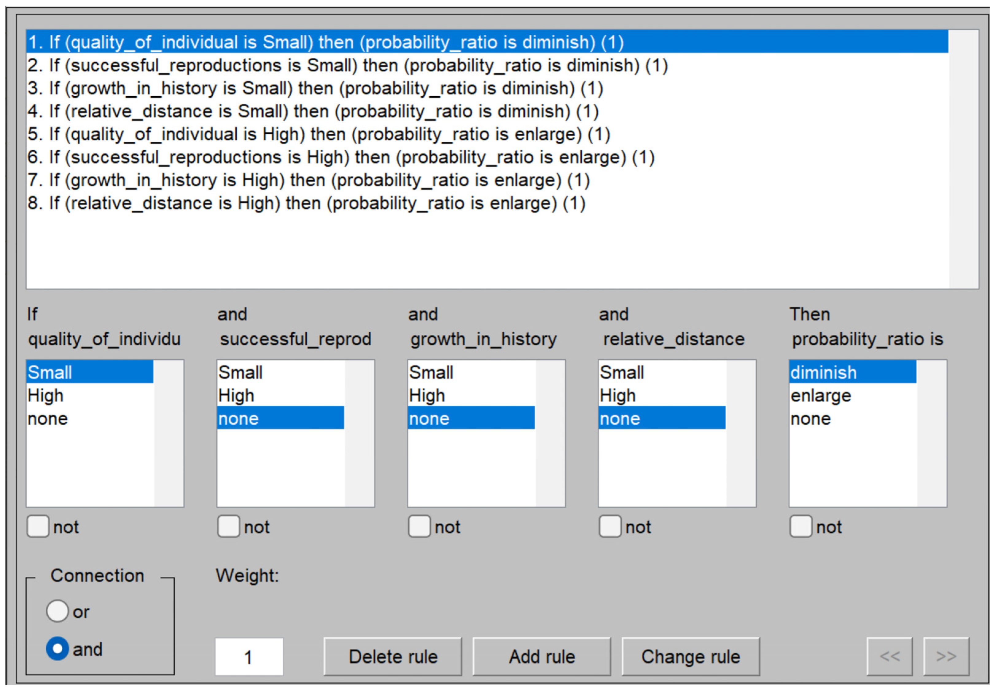
2.1.2. The Rules Base for FLC

A new selection probability is calculated by the FLC for each individual in every generation, based on the following rules:

• Enlarge selection probability for high-quality individuals:
  • Individuals with fitness values above the generation’s average will have their selection probability increased.
  • This prioritization allows such individuals to contribute more offspring, enhancing the algorithm’s ability to exploit existing good solutions.
• Enlarge selection probability for populations with many positive reproductions:
  • Individuals that produce offspring with better fitness than their own will gain higher selection probabilities.
  • This encourages the exploitation of successful reproduction patterns.
• Enlarge selection probability for populations with a high historical growth ratio:
  • If the average fitness value in the current population exceeds the historical average fitness, it suggests evolutionary progress.
  • Increasing selection probability under these conditions enhances exploitation and accelerates convergence.
• Enlarge selection probability when the relative distance to the best solution is small:
  • As the algorithm progresses, the gap between the population’s average fitness and the best found fitness decreases.
  • Increasing selection probability in this final phase focuses the algorithm on refining the best solutions, improving exploitation and convergence.
• Diminish selection probability for low-quality individuals:
  • Individuals with fitness values below the generation’s average will have their selection probability reduced.
  • This limits their contribution to the parent pool, promoting exploitation of better solutions.
• Diminish selection probability for populations with few positive reproductions:
  • Individuals that produce offspring with lower fitness than their own will have their selection probability diminished.
  • This encourages exploration by reducing focus on unsuccessful reproduction patterns.
• Diminish selection probability for populations with a low historical growth ratio:
  • If the population’s average fitness is below the historical average, it indicates a lack of evolutionary progress.
  • Reducing selection probability in such cases focuses resources on better exploitation strategies.
• Diminish selection probability when the relative distance to the best solution is large:
  • In the initial stages, the average fitness of the population is often far from the best found fitness.
  • Reducing selection probability during this phase promotes genetic diversity, enhancing the algorithm’s exploratory capabilities.

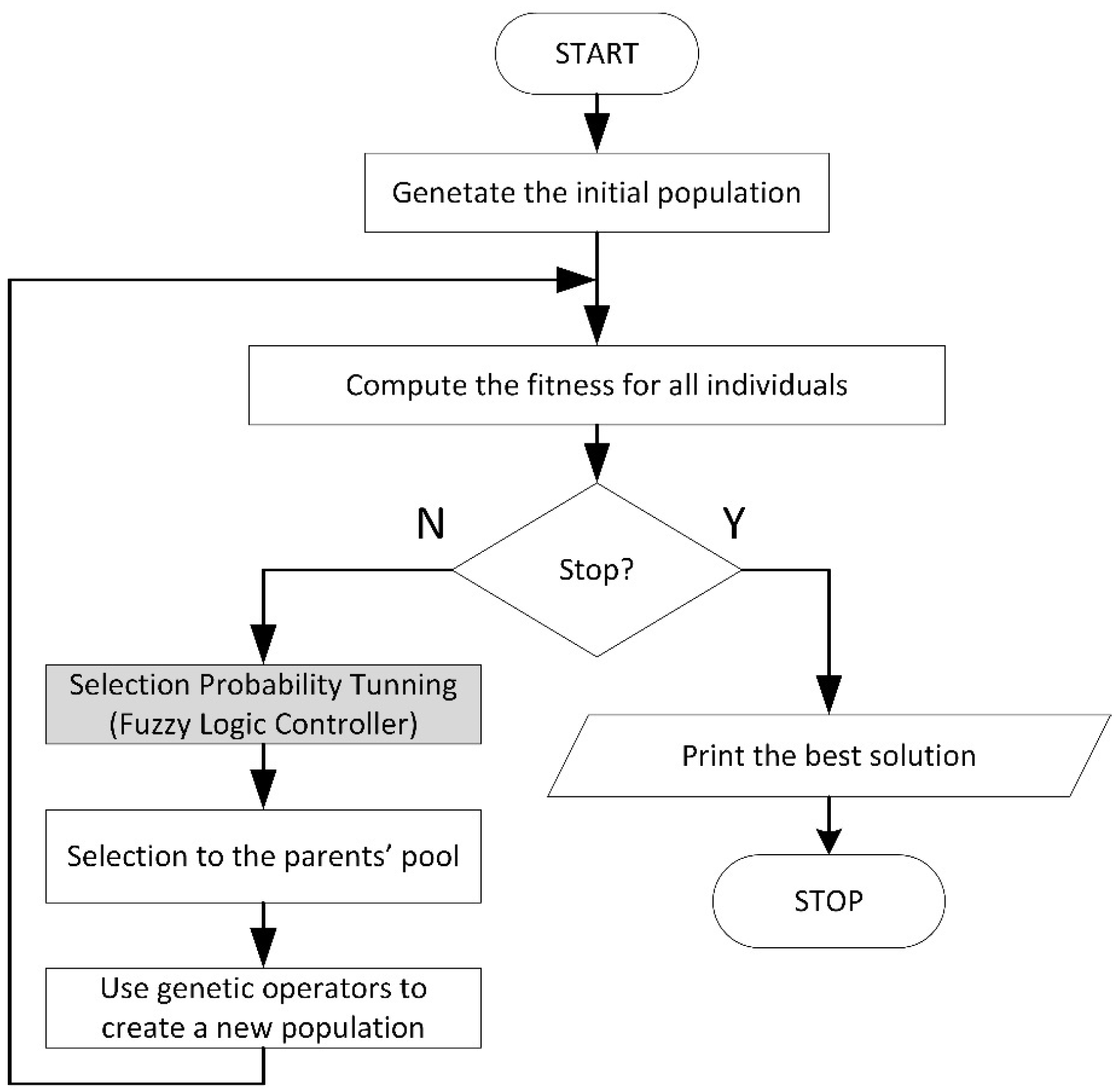
2.1.3. The Modified Evolutionary Algorithm

Figure 1 presents a block diagram of the modified EA, with the FLC block highlighted in gray. Figure 2 illustrates the input and output linguistic variables and their corresponding membership functions used by the FLC.

Algorithm 1 presents the pseudocode of the modified evolutionary algorithm.

Algorithm 1 Adaptive Parameter Evolutionary Algorithm
1	int generation ← 0
2	initialize first population
3	evaluate first population
4	keep best in population
	//Main evolutionary loop
5	while (!termination condition) do
6	generation++
	//Adjust parameters if enough history is available
7	if (generation > history_size) then
8	evaluate estimators for FLC
9	alter selection probability by FLC
10	end if
	//Perform genetic algorithm operations
11	select individuals to parent pool
12	perform crossover and mutation
13	evaluate population
14	apply elitism
15	end while
16	end

2.1.4. The Parameters of Modified Evolutionary Algorithm

Roulette wheel selection is a popular probability-based technique in EAs, used to randomly select parents for reproduction based on their fitness scores. The selection probability of an individual depends directly on its fitness. Fuzzy logic can leverage expert knowledge and information from previous generations to adjust selection pressure and guide the evolutionary process toward desirable regions of the solution space. Fuzzy logic was chosen to control the probability of selection due to its advantages:

−

Human-like decision making: FL-based systems model human decision making, making the control model easier to understand.

−

Simplified modeling of complex problems: FL allows for modeling complex systems without requiring precise mathematical formulations.

−

Robustness to uncertainty: FL-based systems are resistant to small changes in input data or noise, ensuring stable operation under uncertain conditions.

−

Scalability and flexibility: These systems can be easily expanded by adding new rules without requiring a complete redesign, making them adaptable to the problem at hand.

−

Real-time efficiency: FL works well in real-time systems due to its low computational requirements.

Estimators describing an individual’s quality and the population’s historical behaviors are calculated using Formulas (1)–(4), based on data from the current generation and several preceding generations. The tuning of selection probabilities begins with the first generation, where all required historical data are available. The number of generations used for these calculations depends on the history size, a parameter adjustable by the user to tailor the algorithm to the specific problem. The FLC computes the selection probability ratio for all individuals using a predefined formula.

$$ps{\left(i\right)}^{t+1}=ps{\left(i\right)}^t\times psr\left(i\right)$$

(5)

where:

$ps{\left(i\right)}^{t+1}$—selection probability after modification by FLC;

$ps{\left(i\right)}^t$—selection probability before modification by FLC;

$psr\left(i\right)$—selection probability ratio calculated by FLC for individual i.

The value of the selection probability ratio is restricted to 20% of its initial value to prevent rapid fluctuations. The fuzzy logic toolbox on the MATLAB R2024b platform was utilized to develop, simulate, and test the FLC. The FLC is based on the Mamdani model and employs the “center of gravity” method for defuzzification. During initial experiments, data such as the number of successful reproductions, individual fitness values, and the population’s average fitness were collected. This statistical information was used to define the membership functions (MFs) of the input and output linguistic variables (LVs), including their number, shape, and characteristics. The rule database, which is depicted in Figure 3, enables the integration of expert knowledge into the optimization process. It comprises a set of simple rules that allow users to tailor the EA to specific problems by adjusting the selection probability. Additionally, other parameters, such as gene representation, population size, and mutation probability, can also be programmed. Users can customize the history size, the number of MFs, and their shape and properties. The algorithm was implemented in C++ using standard libraries and designed to run on the Windows operating system.

In our experiments, we utilize EAs to explore the search space within an n-dimensional domain ${\Re }^n$. The genes of individuals are represented as fixed-length vectors of real numbers. The fitness function f(x), computed for each individual x, indicates the quality of that individual.

$$f\left(x\right):{\Re }^n\to \Re ,x=\left[x_1,x_2,\dots ,x_n\right],n\in N$$

(6)

A mutation is performed by adding a randomly generated number to the value of each gene in an individual.

$$x_k^{t+1}=x_k^t+N\left(0,\sigma \right),k=1,2,\dots ,n$$

(7)

The mutation process includes mechanisms to ensure that the resulting gene values remain within acceptable domain ranges. The mutation size (σ in Formula (7)) is a parameter of the algorithm that can be adjusted by the user depending on the problem being addressed. The algorithm employs a single-point crossover with a randomly selected crossover point. During this process, all genes (represented as real numbers) of the individuals are exchanged.

In the algorithm, the roulette wheel method is used to select individuals for the parent pool. Other algorithm parameters, such as selection and mutation probabilities, were determined experimentally during preliminary experiments for each benchmark task. The algorithm terminates when the best individual achieves a predetermined fitness value.

The parameters common to all experiments include:

−

population size: 25;

−

crossover probability: 0.8;

−

mutation probability was selected depending on the number of variables in the optimized function so that at least one of the individual’s genes was modified.

2.2. The Set of Test Functions

In a function optimization problem (FOP), the objective is to determine the best or a set of optimal parameters that maximize or minimize a given objective function while adhering to specified constraints. FOPs, owing to their simplicity and the availability of well-documented test functions, are often used as benchmarks to evaluate and compare the performance of various optimization methods, including evolutionary algorithms, metaheuristic algorithms, and other optimization techniques. Several popular approaches for solving FOPs are discussed in the literature, for example, in [23,24,25]. FOPs, with their diverse features encompassing various complexities and characteristics, provide an ideal environment for assessing the impact of tuning the selection probability in EAs. The set of test functions used in the experiments includes functions with a broad range of complexity, differing in difficulty, dimensionality, and the number of local or global optima. These functions include:

−

Selected CEC2015 test functions [26]. All of them are minimization problems, with the minimum shifted to 0 and the search range [−100, 100] for each dimension d. In the experiments, 50 and 100 dimensions were used for the functions CEC_f1, CEC_f2, CEC_f3:

$CEC\_f1\left(x_1,x_2,\dots ,x_d\right)$—high conditioned elliptic function. It is defined as:

$$CEC\_f1\left(x_1,x_2,\dots ,x_d\right)={\displaystyle \sum }_{i=1}^d{\left({10}^6\right)}^{{\displaystyle \frac{i-1}{d-1}}}{x}_i^2$$

(8)

$CEC\_f2\left(x_1,x_2,\dots ,x_d\right)$—cigar function. It is defined as:

$$CEC\_f2\left(x_1,x_2,\dots ,z_d\right)=x_1^2+{10}^6{\displaystyle \sum }_{i=2}^d{x}_i^2$$

(9)

$CEC\_f3\left(x_1,x_2,\dots ,x_d\right)$—discus function. It is defined as:

$$CEC\_f3\left(x_1,x_2,\dots ,x_d\right)={10}^6{x}_1^2+{\displaystyle \sum }_{i=2}^d{x}_i^2$$

(10)

−

$f1\left(x_1,x_2,\dots ,x_d\right)$. The product of 5 to 20 sines has been used to test the algorithm’s ability to determine the exact solution. It is defined as:

$$f1\left(x_1,x_2,\dots ,x_d\right)={\displaystyle \prod }_{i=1}^d\sin \left(x_1\right), x_1,x_2,\dots ,x_d\in \left(0,\pi \right), d=5, 10, 20$$

(11)

−

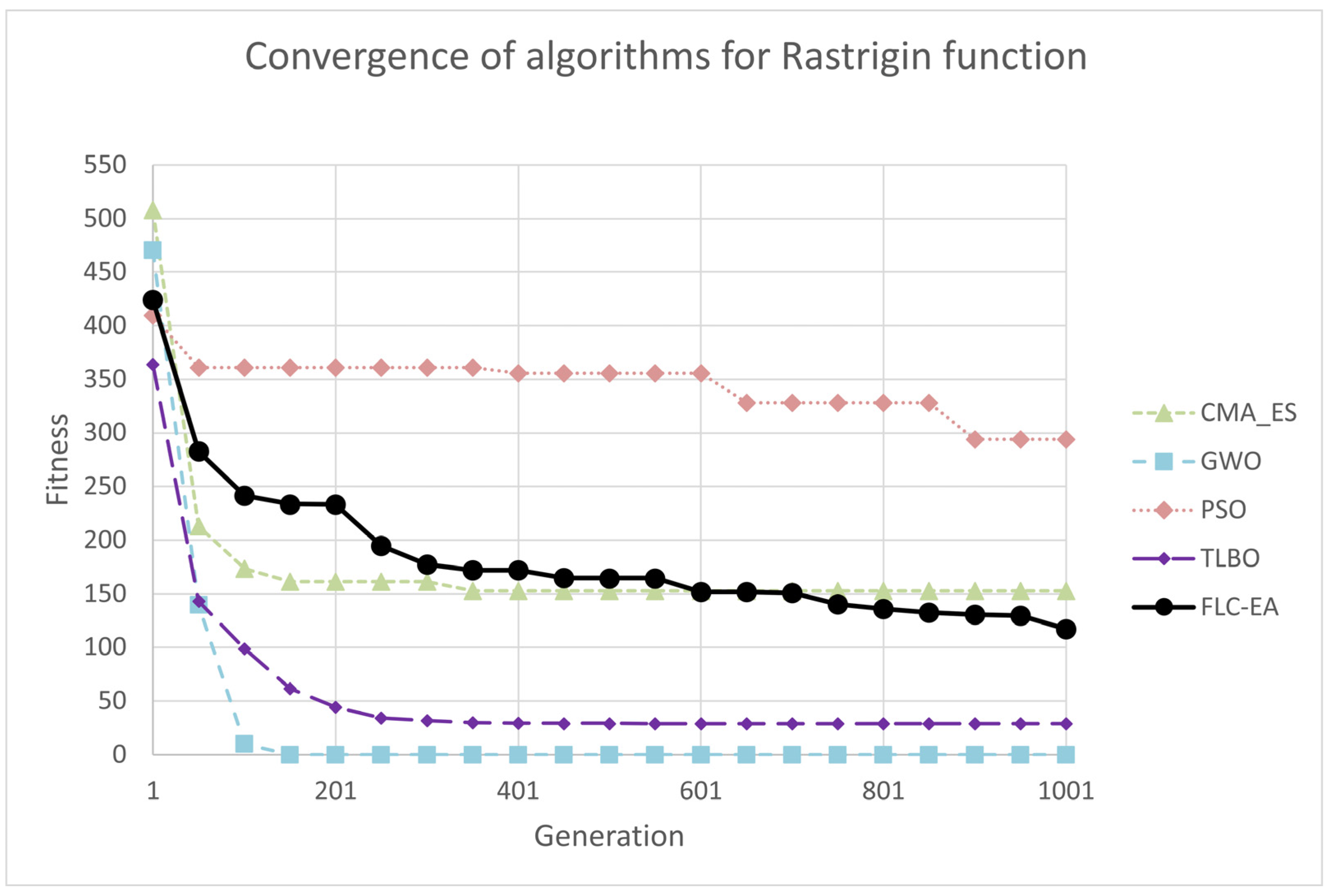
Rastrigin function: It is defined on the domain $x_i\in \left[-5.12, 5.12\right]$, for d = 2, 5, 10 dimensions. The function minimum $f_{Ra}\left(x^{\ast }\right)=0$ is at point $x^{\ast }=\left(0,\dots ,0\right)$. It is defined as:

$$f_{Ra}\left(x\right)=10d+{\displaystyle \sum }_{i=1}^d\left[x_i^2-10\mathit{cos}\left(2\pi x_i\right)\right]$$

(12)

−

Styblinski–Tang function: It is defined for $x_i\in \left[-5, 5\right]$, for all d = 2, 5, 10 dimensions. The minimum of the function $f_{ST}\left(x\right)=-39.16599d$ is located at the point $x^{\ast }=\left(-2.903534,\dots ,-2.903534\right)$. It is defined as:

$$f_{ST}\left(x\right)={\displaystyle \frac{1}{2}}+{\displaystyle \sum }_{i=1}^d\left[x_1^4-16x_i^2+5x_i\right]$$

(13)

−

Rosenbrock function: It is defined for 2 dimensions in domain $x_i\in \left[-5, 10\right]$, for each dimension. The function minimum $f_{Ro}\left(x\right)=0$ is at point $x^{\ast }=\left(1,\dots ,1\right)$. It is defined as:

$$f_{Ro}\left(x\right)={\displaystyle \sum }_{i=1}^{d-1}\left[100{\left(x_{i+1}-x_i^2\right)}^2+{\left(x_{i-1}\right)}^2\right]$$

(14)

−

Shubert function: It is defined for 2 dimensions in domain $x_i\in \left[-2, 2\right]$, for each dimension. The function minimum $f_{Ro}\left(x\right)=-186.7309$. It is defined as:

$$f_{Sh}\left(x\right)=(\sum _{i=1}^{5}i cos\left(\left(i+1\right)x_1+i\right))(\sum _{i=1}^{5}i cos(\left(i+1\right)x_2+i))$$

(15)

−

$f2\left(x_1,x_2\right)$. A simple function of two variables in domain $x_i\in \left[0, \pi \right]$, for each dimension. The function maximum $f2\left(x^{\ast }\right)=1.6$ is at point $x^{\ast }=\left({\displaystyle \frac{\pi }{2}},{\displaystyle \frac{\pi }{2}}\right)$. It is defined as:

$$f2\left(x_1,x_2\right)=(\sin \left(x_1\right)+0.6\times \sin \left(20\times x_1\right))\times sin\left(x_2\right)$$

(16)

−

$f3\left(x_1,x_2\right)$. The very complex function used to test the algorithm’s ability to find a global optimum and avoid local optima. The function maximum $f3\left(x^{\ast }\right)=2.5$ is at point $x^{\ast }=\left(50,50\right)$. It is defined as:

$$f3\left(x_1,x_2\right)={\displaystyle \sum }_{i=1}^7{h}_i\times e^{-{\mu }_1\times {\left(x_1-x_{i1}\right)}^2+{\left(x_2-x_{2i}\right)}^2}$$

(17)

where:

$h_1=1.5,h_2=h_3=h_4=1,h_5=h_6=2,h_7=2.5$;

${\mu }_1={\mu }_2={\mu }_3={\mu }_4={\mu }_5={\mu }_6={\mu }_7=0.01$;

$\begin{array}{l}\left(x_{11},x_{12}\right)=\left(5,5\right), \left(x_{21},x_{22}\right)=\left(5,30\right), \left(x_{31},x_{32}\right)=\left(25,25\right), \left(x_{41},x_{42}\right)=\\ \left(30,5\right), \left(x_{51},x_{52}\right)=\left(50,20\right), \left(x_{61},x_{62}\right)=\left(20,50\right), \left(x_{71},x_{72}\right)=\left(50,50\right)\end{array}.$

2.3. Real-World Test Problem

In a multiple-objective optimization problem (MOP), multiple objective functions must be optimized simultaneously, often with competing or conflicting objectives. Improving one objective may result in the degradation of another. The goal of the MOP is to identify a solution or a set of solutions where no other solution is superior in all objectives simultaneously. This solution set, commonly referred to as the Pareto optimal solution, represents the best achievable trade-offs among all the objective functions. Each solution in the Pareto set is non-dominated, meaning that no other solution in the set is better across all objectives.

2.3.1. Connected Facility Location Problem

The connected facility location problem (ConFLP) [9,27] serves as a practical example of an MOP. The primary goal of the ConFLP is to determine the optimal placement of facilities (or network nodes) and establish the connections between these facilities and demand points (e.g., computer terminals). The ConFLP’s objectives include minimizing construction or operational costs while maximizing coverage or minimizing total service distance. The problem is inherently complex due to the need to balance multiple conflicting goals and objective functions, with each objective contributing differently to the overall quality of the solution. Additionally, the correlation between network node placement and terminal connectivity further complicates the problem. Traditional single-objective optimization methods are inadequate for solving the ConFLP. However, EAs offer a robust approach for handling this type of problem. The ConFLP model integrates three classical problems fundamental to designing an efficient computer network topology:

−

Network Nodes Location Problem: Network nodes must be placed within a given geographic area to minimize the total length of communication links between nodes and terminals. Placing network nodes closer to computer terminals reduces the total communication distance, leading to decreased latency and improved overall network performance. The placement must also consider real-world constraints such as physical barriers, existing infrastructure, and geographic boundaries.

−

Network Nodes Number Problem: The number of network nodes should be minimized to reduce infrastructure costs and simplify network management, while ensuring effective coverage and connectivity. A smaller number of nodes may lead to longer distances between terminals and nodes, potentially increasing communication delays and causing network congestion.

−

Terminal Assignment Problem: Each computer terminal must be assigned to its nearest network node to minimize the total link length between nodes and terminals. This assignment involves solving the nearest neighbor problem efficiently while ensuring proper load balancing to prevent overloading specific nodes.

Formally, ConFLP within a given 2D geographic area can be stated as:

$$\left\{\begin{array}{l}\min f_1\left(x_1,y_1,x_2,y_2,\dots ,x_n,y_n\right)\\ \min f_2(n,x_1,y_1,x_2,y_2,\dots ,x_n,y_n)\\ subject to:cost and length constraints\end{array}\right.$$

(18)

where:

$f_1$—This function represents the total link length between network nodes and computer terminals. It could be expressed as the sum of the distances between each computer terminal and its assigned network node.

$f_2$—This function assigns each computer terminal to a specific network node. This could be based on criteria like the shortest distance, load balancing, or other optimization goals.

$(x_{1,}{y}_1,x_2,y_2,\dots ,x_n,y_n)$—These are the coordinates of the network nodes, where A represents the 2D area in which these nodes are positioned.

$1\le n\le n_{max}$—n represents the current number of network nodes.

In a given service area A, with n network nodes and known locations of computer terminals (x,y), the objective is to determine the optimal placement of network nodes and assign terminals to these nodes to minimize the total link length between terminals and nodes. Designing computer networks presents several practical challenges. Cisco’s hierarchical model for local networks divides the network into three layers: core, distribution, and access. This model emphasizes reducing the number of network nodes between the network’s extreme points. The Spanning Tree Protocol (STP) was developed and implemented to prevent loops in switched networks with redundancy. To ensure stability, STP mandates that no more than seven nodes exist between any two endpoints. This limitation must be respected when determining network node placement and terminal associations. The constraints introduced by Cisco’s hierarchical design model and STP add significant complexity to the network design process.

The proposed evolutionary algorithm can find feasible solutions that not only minimize costs but also comply with the operational and protocol-driven constraints of the network. To achieve this, an additional constant C is introduced to transform the decreasing fitness function into an increasing one. This transformation ensures that solutions with lower total link lengths correspond to higher fitness function values. The constant C must be sufficiently large to ensure that the fitness value remains positive. Both the value of C and the stopping criterion are determined experimentally, depending on the problem’s complexity and the desired solution quality. Potential solutions to the problem are encoded using two tables, representing both node positions and terminal-node associations:

−

Node positions by geographical coordinates: This table contains the coordinates of each network node. The number of genes in an individual equals the number of network nodes (n). Each gene consists of two real numbers, representing the x and y coordinates of a node.

−

Terminal-node associations: This table assigns each terminal to a network node using integers. The number of genes in an individual equals the number of terminals. A value i at position k indicates that terminal k is connected to node i.

Different mutation probabilities are set experimentally for the two tables to control the balance between exploration and exploitation, depending on the task size.

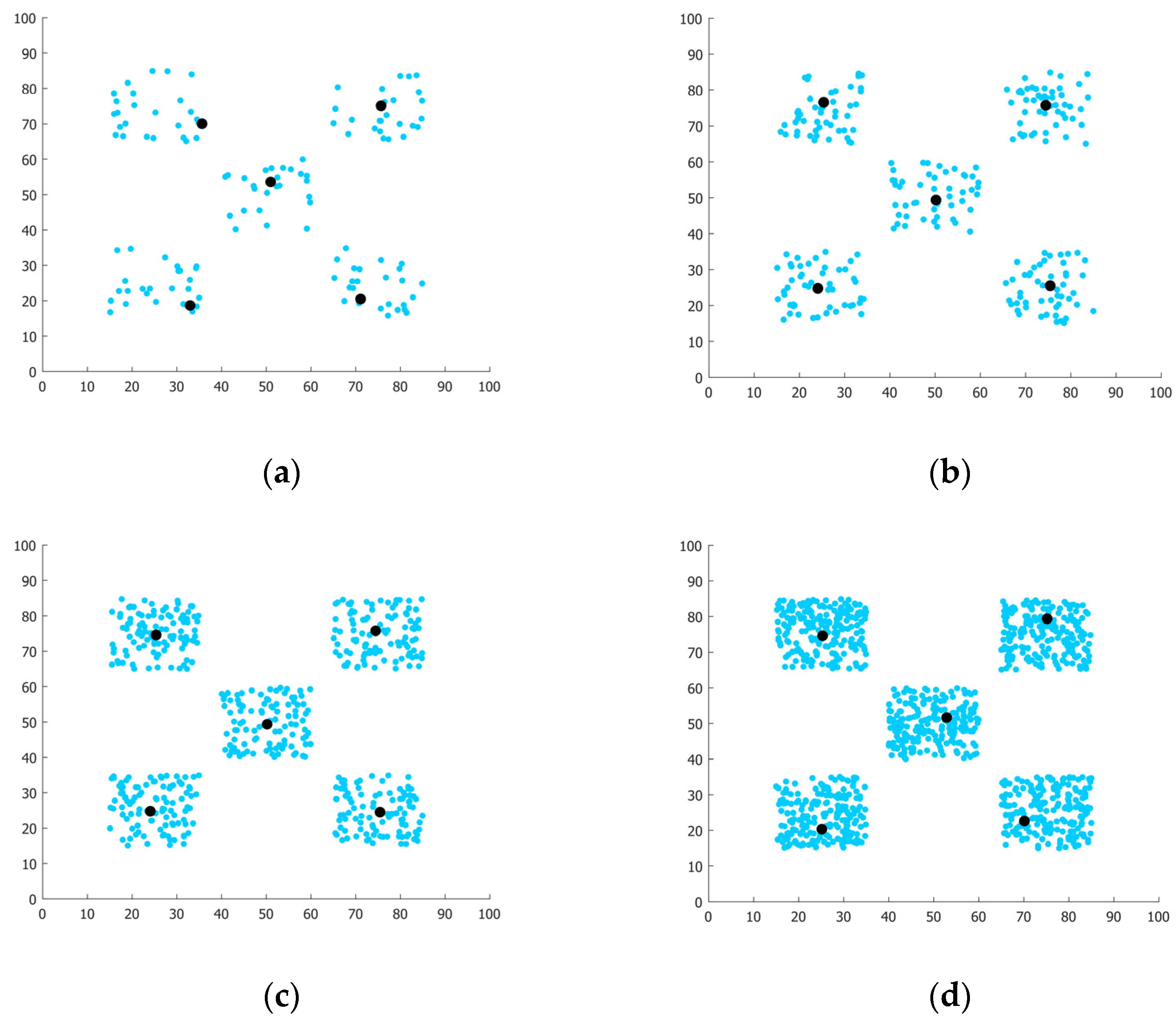
2.3.2. Clustering Problem

The clustering problem involves assigning objects to groups of similar objects, called clusters, based on their features. Each object is described in d-dimensional space. The goal is to group the objects into k clusters such that similar objects are assigned to the same cluster. Typically, the Euclidean distance between pairs of objects is used as a similarity measure, although other measures can also be applied. Clustering must satisfy the following constraints: each object can be assigned to only one cluster at a time, and each cluster must contain at least one object.

3. Results

A set of computational experiments was conducted to evaluate the efficiency, performance, and convergence of the proposed FLC-EA algorithm compared to a standard evolutionary algorithm (EA). The experiments, divided into several stages, were performed on a system with the following specifications: an Intel i7 processor supported by 8 GB of RAM. During the initial phase, the algorithm’s parameters—such as population size, selection probability, and mutation probability—were fine-tuned to best fit the test tasks.

3.1. Experiments on a Simple, Monotone Function

In the first stage of the experiments, the primary goal was to assess the efficiency of the algorithms in finding the exact optimal value. A simple monotonic function f1 with 5, 10, and 20 variables was selected. The results of the proposed FLC-EA algorithm, including performance and efficiency, were compared with those of the standard EA algorithm [5].

Table 1. Results for the optimization of the f1 function: the number of generations and the running time, including the minimum, average, maximum, and standard deviation, respectively.

Algorithm	Dimension Size	The Number of Generations				The Running Time (s)
		Min Value	Average Value	Max Value	σ	Min Value	Average Value	Max Value	σ
EA	5	4693	10,898.5	24,386	5708.4	0.26	0.540	1.22	0.278
	10	21,481	46,591.7	72,196	14,013.2	1.80	3.666	5.44	1.072
	20	207,270	250,109	345,307	42,042.2	29.05	35.716	49.38	6.392
FLC-EA	5	2114	6188.1	14,732	3840.1	0.13	0.334	0.61	0.151
	10	6790	13,363.1	21,539	5001.2	0.68	1.026	1.49	0.299
	20	37,795	45,190.7	58,356	7074.3	4.74	6.134	8.33	1.264

presents the outcomes from 30 runs of each algorithm (FLC-EA and EA), including the number of generations, the algorithm’s runtime until the stopping criterion was met, and their standard deviations.

Results from the first-stage experiments on easy-to-optimize functions confirm that the FLC-EA algorithm requires 43% to 81% fewer generations and 38% to 82% less runtime compared to the standard evolutionary algorithm. Although the inclusion of the FLC introduces additional computational effort, this overhead is expected to be offset when applied to computationally complex functions in multidimensional environments, where further performance improvements are anticipated.

3.2. Experiments on High-Dimensional Benchmark Functions from CEC2015

In the second stage of experiments, a set of high-dimensional benchmark functions from CEC2015 was analyzed.

Table 2. Results for the optimization of the CEC functions (CEC_f1, CEC_f2, and CEC_f3): the number of generations and the running time, including the minimum, average, maximum, and standard deviation.

Algorithm	Function	Dimension Size	The Number of Generations				The Running Time (s)
			Min Value	Average Value	Max Value	σ	Min Value	Average Value	Max Value	σ
EA	CEC_f1	50	31,510	33,922.7	35,905	1358.5	6.5	6.96	7.4	0.30
		100	37,877	40,511.2	43,039	1891.2	18.0	19.18	20.7	0.77
	CEC_f2	50	863,016	1,046,476.0	1,210,955	97,090.6	144.0	175.10	201.0	16.34
		100	858,736	904,124.2	1,056,167	56,535.3	259.0	273.10	318.0	16.79
	CEC_f3	50	31,464	33,340.3	36,243	1816.4	5.4	6.04	7.3	0.61
		100	60,587	66,627.7	77,322	4766.8	18.7	20.73	23.6	1.81
FLC-EA	CEC_f1	50	15,537	17,815.7	18,904	1134.8	3.1	3.83	4.8	0.48
		100	22,079	25,037.3	27,040	1344.6	9.3	11.03	11.9	0.75
	CEC_f2	50	159,626	203,278.7	259,870	30,706.9	26.5	33.67	45.0	5.13
		100	157,404	167,989.9	188,238	10,955.1	46.6	51.27	55.6	3.25
	CEC_f3	50	15,859	18,180.4	20,146	1370.4	2.5	3.13	3.51	0.25
		100	25,334	28,594.4	30,701	1646.9	7.3	9.42	10.85	1.01

presents the outcomes from 30 runs of each algorithm (FLC-EA and EA) for optimizing the CEC_f1, CEC_f2, and CEC_f3 functions, along with their standard deviations.

Tests on multidimensional CEC2015 functions confirm the superiority of the proposed FLC-EA algorithm over the standard EA, both in terms of the number of generations (38% to 81% fewer) and runtime (42% to 81% faster).

3.3. Test on a Set of Complex, Non-Trivial, and Difficult-to-Optimize Functions

In the third stage of experiments, a set of complex, non-trivial, and difficult-to-optimize functions was analyzed.

Table 3. Results for the optimization of difficult-to-optimize functions (Rastrigin, Styblinski–Tang, Rosenbrock, and Shubert): the number of generations and the running time, including the minimum, average, maximum, and standard deviation.

Algorithm	Function	Dim. Size	The Number of Generations				The Running Time (s)
			Min Value	Average Value	Max Value	σ	Min Value	Average Value	Max Value	σ
EA	Rastrigin	2	4683	8841.4	20,323	4544.5	0.16	0.288	0.54	0.121
		5	19,775	50,067.1	84,228	21,334.4	0.91	2.365	3.98	0.981
		10	62,918	134,660.6	329,182	80,650.2	5.03	10.612	25.64	6.230
	Styblinski–Tang	2	977	2094.5	3711	1048.5	0.05	0.085	0.12	0.022
		5	3321	10,465.7	13,956	3941.4	0.20	0.560	0.73	0.196
		10	20,455	39,374.8	67,366	17,382.1	1.48	2.841	4.79	1.236
	Rosenbrock	2	2626	5091.1	7652	1885.0	0.08	0.138	0.19	0.037
	Shubert	2	4212	9056.4	16,943	4164.9	0.23	0.449	0.89	0.206
FLC-EA	Rastrigin	2	419	3040.4	9632	2785.2	0.07	0.144	0.33	0.075
		5	6597	19,526.4	53,574	15,501.5	0.35	0.914	2.82	0.773
		10	4696	31,862.5	56,953	16,612.2	0.43	2.266	3.92	1.092
	Styblinski–Tang	2	472	1215.1	2599	647.6	0.05	0.198	0.54	0.141
		5	324	2238.7	4036	1238.3	0.08	0.178	0.24	0.057
		10	4924	10,863.9	19,091	4289.8	0.39	0.758	1.54	0.331
	Rosenbrock	2	322	2333.5	4973	1406.6	0.07	0.127	0.18	0.034
	Shubert	2	1343	3924.2	7654	2115.6	0.13	0.368	1.24	0.342

presents the outcomes from 30 runs of each algorithm for optimizing the Rastrigin, Styblinski–Tang, Rosenbrock, and Shubert functions, along with their standard deviations.

Tests on computationally complex, variable-dimension functions confirm the effectiveness of the FLC-EA algorithm for such tasks. The proposed algorithm completes execution after significantly fewer generations: approximately 60% to 76% fewer for the Rastrigin function, 40% to 78% fewer for the Styblinski–Tang function, 54% fewer for the Rosenbrock function, and 56% fewer for the Shubert function. However, for the Styblinski–Tang function in a two-dimensional domain, the algorithm’s runtime is longer. This may be due to the standard EA handling this function efficiently, with the reduced number of generations failing to offset the computational overhead introduced by the additional FLC mechanism. In all other tasks, the FLC-EA algorithm demonstrated shorter runtimes: approximately 50% to 78% faster for the Rastrigin function, 68% to 73% faster for the Styblinski–Tang function, 7% faster for the Rosenbrock function, and 18% faster for the Shubert function, compared to the standard EA.

3.4. Test on Multi-Modal Functions

In the fourth stage of the experiments, the performance of the algorithm was evaluated on multi-modal functions f2 and f3. We assessed the ability of the algorithms to escape local optima in these multi-modal functions. The f3 function is particularly challenging due to the complexity of its landscape. The algorithm begins with an initial population centered around a local maximum at point (5, 5) with a value of 1.5. The optimization process requires the algorithm to navigate through valleys and bypass multiple local maxima (values 1.0 and 2.0) in order to reach and populate the global maximum region at point (50, 50) with a value of 2.5.

Table 4. Optimization results for the f2 and f3 functions: the number of generations and the running time, including the minimum, average, maximum, and standard deviation.

Algorithm	Function	The Number of Generations				The Running Time (s)
		Min Value	Average Value	Max Value	σ	Min Value	Average Value	Max Value	σ
EA	f2	1124	3983.4	8690	2569.03	0.07	0.178	0.33	0.1004
	f3	8360	36,091.7	75,261	23,355.20	0.38	1.537	3.23	0.9683
FLC-EA	f2	248	1482.8	3466	1022.07	0.08	0.122	0.21	0.0426
	f3	594	13,942.1	32,880	9477.15	0.13	0.759	1.62	0.4385

presents the outcomes from 30 runs of the FLC-EA and EA algorithms, including the number of generations and the runtime until the stopping criterion is met, as well as their standard deviations.

The experiments on the f2 and f3 functions confirm the improved exploration capability of the FLC-EA algorithm compared to the standard EA. The proposed algorithm completes tasks after 61% and 62% fewer generations, and in approximately 31% and 50% shorter running times for the f2 and f3 functions, respectively.

3.5. Comparition of Proposed Method to Reinforcement-Learning-Based Algorithm

Reinforcement learning (RL) [28,29] is a branch of machine learning where an intelligent agent learns to make decisions by interacting with an environment. Unlike supervised learning, RL does not require labeled input–output pairs to be presented to the agent. Instead, the agent learns by receiving feedback in the form of rewards or penalties based on its actions. The agent’s goal is to learn a policy that maximizes cumulative rewards over time. This policy can be either deterministic (always choosing the best action) or stochastic (choosing actions probabilistically). A significant challenge in RL is balancing exploration (trying new actions to discover rewards) and exploitation (using known actions to maximize immediate rewards). RL algorithms are highly effective and widely applied in various domains:

−

Gaming: training artificial agents for games like chess, Go, and video games.

−

Robotics and autonomous vehicles: teaching robots or self-driving cars to navigate and perform tasks.

−

Healthcare: optimizing treatment plans and aiding in drug discovery.

−

Finance: portfolio optimization and automated trading strategies.

Reinforcement learning (RL) has been successfully applied to solve numerous real-world technical problems. For example, it has been used for parameter estimation of photovoltaic models to enhance the efficiency and performance of solar energy systems [30]. Teaching-learning-based optimization (TLBO) is a population-based metaheuristic algorithm inspired by the teaching and learning interactions in a classroom [31]. In this approach, a “teacher” guides the “students” (candidate solutions) to improve their performance, while students further refine their understanding through mutual interactions. TLBO, available in publication [32] for MATLAB, will serve as a benchmark for evaluating the convergence of the FLP-EA algorithm, providing a standard for comparison in terms of convergence to optimum.

The experiment aims to compare the convergence of the FLC-EA and TLBO algorithms in solving FOP tasks.

Table 5. The convergence of algorithm: the number of generations, including the minimum, average, maximum, and standard deviation.

Algorithm	Function	Size	The Number of Generations
			Min Value	Average Value	Max Value	σ
FLC-EA	f1	2	2114	6188.1	14,732	3840.1
		5	6790	13,363.1	21,539	5001.2
		10	37,795	45,190.7	58,356	7074.3
	CEC_f1	50	15,537	17,815.7	18,904	1134.8
		100	22,079	25,037.3	27,040	1344.6
	CEC_f2	50	159,626	203,278.7	259,870	30,706.9
		100	157,404	167,989.9	188,238	10,955.1
	CEC_f3	50	15,859	18,180.4	20,146	1370.4
		100	25,334	28,594.4	30,701	1646.9
	Rastrigin	2	419	3040.4	9632	2785.2
		5	6597	19,526.4	53,574	15,501.5
		10	4696	31,862.5	56,953	16,612.2
	Styblinski–Tang	2	472	1215.1	2599	647.6
		5	324	2238.7	4036	1238.3
		10	4924	10,863.9	19,091	4289.8
	Rosenbrock	2	322	2333.5	4973	1406.6
	Shubert	2	1343	3924.2	7654	2115.6
	f2	2	248	1482.8	3466	1022.0
	f3	2	594	13,942.1	32,880	9477.1
TLBO	f1	2	19	24.9	31	2.4
		5	52	70.6	90	12.0
		10	201	248.3	339	37.8
	CEC_f1	50	48	50.7	53	1.4
		100	54	54.9	56	0.8
	CEC_f2	50	30	31.4	33	1.1
		100	33	34.4	36	1.2
	CEC_f3	50	33	35.8	38	1.4
		100	36	38.2	40	1.5
	Rastrigin	2	4	15.4	74	3.6
		5	145	784.2	4646	1310.3
		10 *	220	1659.7	4715	1443.8
	Styblinski–Tang	2	10	15.4	21	3.6
		5 *	21	40.4	81	18.4
		10 **	-	-	-	-
	Rosenbrock	2	36	64.9	97	19.9
	Shubert	2	32	40.8	48	5.1
	f2	2	26	42.2	75	13.1
	f3	2	10	17.6	31	6.5

* Algorithm failed to complete the task at least once; ** algorithm failed to complete the task.

presents the results from 30 runs of the FLC-EA and TLBO algorithms, including the number of generations required to meet the stopping criterion and their corresponding standard deviations.

The convergence of the FLC-EA algorithm depends on the type of problem being addressed. For function optimization problems, TLBO generally requires much fewer generations across all considered functions. However, in some tasks, TLBO got stuck in local optima.

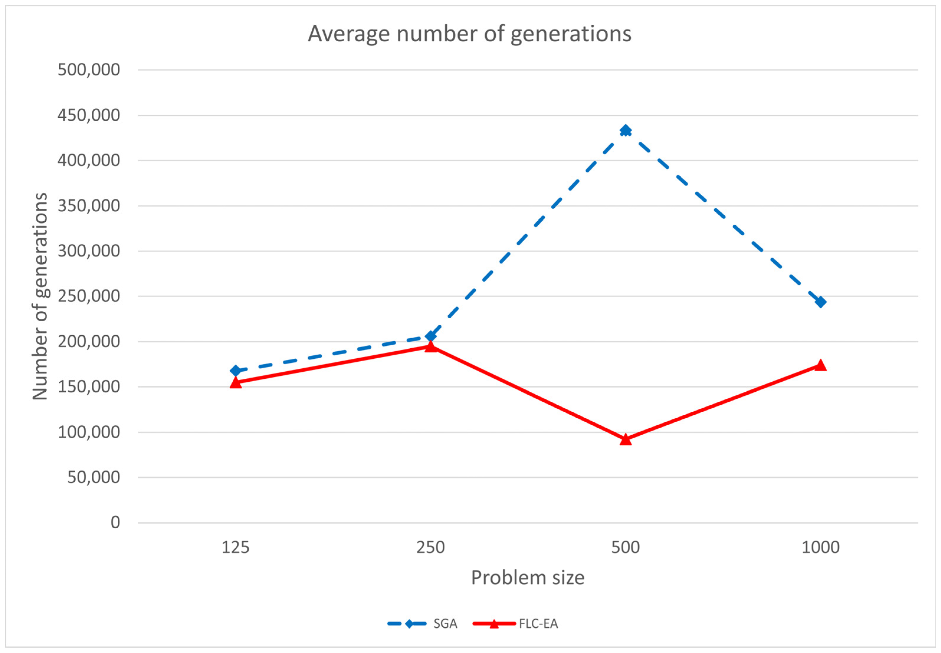
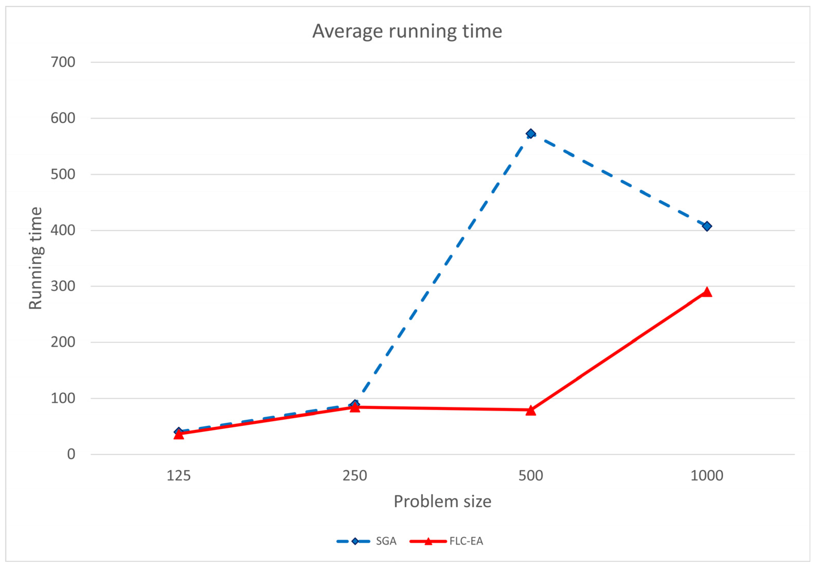
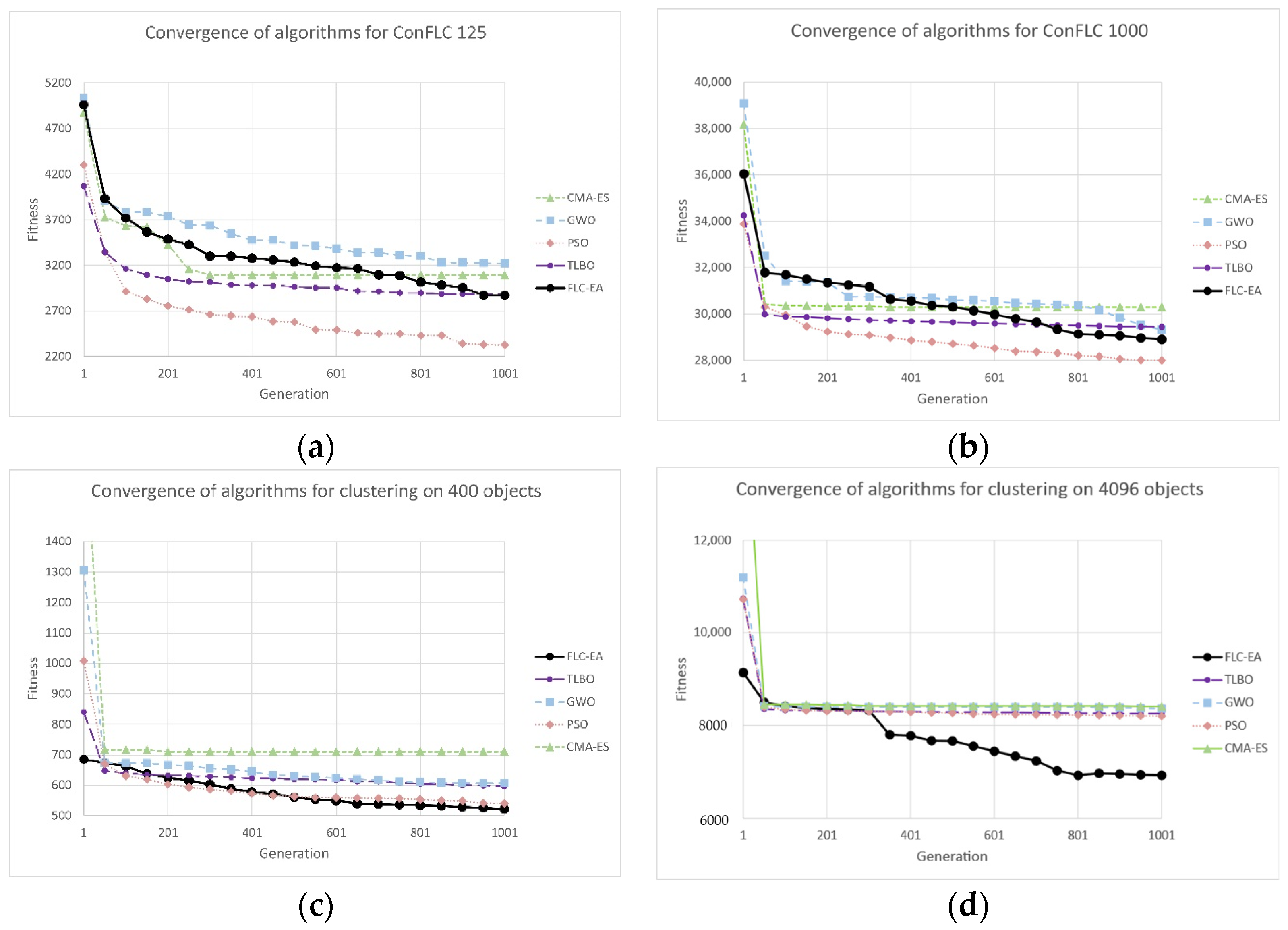
3.6. Test of Algorithm’s Performance on Real-World ConFLP Problem

This experiment aims to verify the performance and effectiveness of an EA supported by an FLC in solving the ConFLP and to compare results to the SGA algorithm [5]. The test setup involves solving a set of tasks with from 125 to 1000 computer terminals, grouped into 5 equal-sized clusters within a 100 by 100 area.

Table 6. Optimization results for ConFLP: the number of generations, including the minimum, average, maximum, and standard deviation.

Algorithm	Problem Size	Constant C	Stop Criterion	The Number of Generations
				Min Value	Average Value	Max Value	σ
SGA	125	7500	6300	48,010	167,594.6	285,740	0.53 × 1011
	250	15,000	13,150	92,350	205,769.3	483,001	1.74 × 1011
	500	30,000	25,000	213,906	433,440.2	1,092,699	6.51 × 1011
	1000	120,000	47,000	152,301	25,6785.5	641,331	1.79 × 1011
FLC-EA	125	7500	6300	41,761	96,255.4	141,282	0.12 × 1011
	250	15,000	13,150	49,010	121,622.1	176,979	0.16 × 1011
	500	30,000	25,000	28,733	87,851.2	207,987	0.21 × 1011
	1000	120,000	47,000	131,543	170,097.9	214,802	0.49 × 1011

and

Table 7. The results for optimization ConFLP: the running time, including the minimum, average, maximum, and standard deviation.

Algorithm	Problem Size	Constant C	Stop Criterion	The Running Time (s)
				Min Value	Average Value	Max Value	σ
SGA	125	7500	6300	11.5	40.26	69.2	2941.27
	250	15,000	13,150	40.0	89.16	207.0	33,041.66
	500	30,000	25,000	224.0	573.13	2069.2	2,981,111.76
	1000	120,000	47,000	253.0	426.85	1066.0	496,622.85
FLC-EA	125	7500	6300	14.9	34.76	53.0	1506.59
	250	15,000	13,150	39.7	81.55	110.2	5455.62
	500	30,000	25,000	44.1	125.59	285.9	38,356.11
	1000	120,000	47,000	310.2	404.61	509.9	29,700.81

show the outcomes from 30 runs of the FLC-EA and SGA algorithms for ConFLP, including the number of generations, the algorithms’ running times until the stopping criterion is met, and their standard deviations.

Figure 4 and Figure 5 present the average running time and the number of generations to the stopping criterion of the FLC-EA and SGA algorithms for ConFLP, respectively.

Figure 6 presents an example distribution of computer terminals and network nodes after optimization for a task with 125 to 1000 terminals. In the task with 500 terminals, the standard SGA performed significantly worse than the FLC-EA algorithm. This disparity may be due to the specific terminal layout and the setting of the stopping criterion near the optimal value. The FLC-EA algorithm completed the tasks significantly faster and required fewer generations, primarily due to its ability to dynamically adapt parameters.

The FLC-EA algorithm not only requires fewer generations to find a solution but also demonstrates reduced running times across all test sizes (from 125 to 1000 terminals), compared to the standard SGA.

3.7. Test of Algorithm’s Performance on Clustering Problem

A dataset from The Fundamental Clustering Problems Suite [33] was selected as a benchmark. The experiment utilized two-dimensional tasks containing between 400 and 4096 objects and involving 2 to 3 clusters. The stopping criterion was based on minimizing the sum of the distances of objects from their respective centroids. This criterion value was determined for each task during preliminary experiments.

Table 8. The best results of all runs obtained by algorithms in tests on selected benchmarks.

Problem name	Algorithm	Lsun	TwoDiamonds	WingNut	EngyTime
Number of objects		400	800	1070	4096
Number of clusters		3	2	2	2
Number of dimensions		2	2	2	2
Stop criterion		600	820	1300	8395
Number of generations to stop criterion	EA	22,849	3851	11,642	19,621
	FLC-EA	6056	2916	2350	1350
Running time to stop criterion [s]	EA	18.8	6.5	23.7	158.6
	FLC-EA	6.5	4.1	8.2	22.5

presents the outcomes from 30 runs of each algorithm for optimizing clustering problems, with sizes ranging from 400 to 4096 objects.

The FLC-EA algorithm requires fewer generations to converge to a solution and demonstrates reduced running times across all test sizes compared to the standard EA.

3.8. Evaluation Algorithm’s Convergence to Global Optima

The fifth stage of the experiments focuses on evaluating the FLC-EA algorithm’s convergence to global optima using the Rastrigin function in a 30-dimensional space. To validate the performance of FLC-EA, its results were compared with three established optimization methods: the covariance matrix adaptation evolution strategy (CMA-ES), as detailed in publication [34]; the Grey Wolf Optimizer (GWO), as introduced in publication [35]; the particle swarm optimization (PSO), as described in publication [36]; and teaching-learning-based optimization (TLBO), as described in publication [32]. For this comparison, implementations of CMA-ES, GWO, and PSO within the MATLAB environment were utilized, ensuring a consistent and fair evaluation across all algorithms. Figure 7 and Figure 8 present the convergence behaviors of the algorithms, showing the best individual’s fitness value after a fixed number of generations.

The convergence on the 30-dimensional Rastrigin function of the FLC-EA algorithm is better than CMA_ES and PSO and worse than GWO and TLBO. However, for real-world problems such as ConFLP and clustering tasks, which involve significantly more complex function optimization, FLC-EA converges faster overall, but is slightly slower in clustering tasks compared to PSO. In the initial generations, CMA-ES, GWO, PSO, and TLBO demonstrate better convergence than FLC-EA; however, FLC-EA outperforms them in later generations.

4. Discussion

The fuzzy logic controller can leverage data from previous generations to adjust the selection probability in evolutionary algorithms dynamically. It effectively balances the trade-off between exploration and exploitation within the search space, enhancing the algorithm’s convergence. A wide range of experiments on function optimization problems of varying complexity and dimension size confirm that the new FLC-EA algorithm successfully solves all tasks presented in the benchmark.

The FLC-EA system offers a few advantages when solving complex optimization problems:

−

Transparency: Fuzzy logic introduces a transparent, easy-to-interpret method for modeling and expressing human knowledge and strategies within the evolutionary process. The use of simple IF-THEN rules enables both experts and non-experts to understand and engage in designing algorithms to solve optimization processes.

−

Incorporating human expertise: Fuzzy logic enables the integration of domain-specific knowledge directly into the optimization process. Experts can encode their knowledge into the fuzzy rule base and guide the EA to align with human goals and constraints. This enhances the relevance of the optimization results and their consistency with the user’s expectations.

−

Robustness and adaptability: The FLC-EA system is better equipped to handle a wide range of benchmarks and real-world problems. It can adapt the fuzzy rule base or membership functions to changing problem constraints or user requirements.

−

Human–machine collaboration: The transparency and interpretability of fuzzy logic foster effective collaboration between humans and the optimization system. Experts can actively participate in refining rules and strategies, leading to more effective outcomes in complex decision-making processes aligned with user goals.

Exploration and exploitation are conflicting objectives in the search process, leading to certain weaknesses and limitations of the FLC-EA algorithm. Parameter tuning in EAs is a critical aspect of their design, and the following challenges are particularly notable:

−

Time-consuming process of development: Tuning FLC parameters, such as the rule database, the number, and the shape of membership functions, is a complex task. This complexity arises from the high dimensionality of the problem, the size of the dataset, and the intricate interactions between various parameters.

−

Computational expense: FLC parameter tuning often requires extensive experimentation, which can be both time consuming and resource intensive. Developers must evaluate numerous configurations and rely on trial-and-error methods, particularly when using manual tuning approaches. This can delay project timelines and significantly increase the costs of software development.

−

High resource requirements for automated tuning: While automated tuning techniques are generally more efficient than manual methods, they often demand substantial computational resources. This is especially true for complex problems, making such methods expensive and potentially inaccessible in resource-constrained environments.

−

Lack of reproducibility: The parameter tuning process can introduce variability in model performance, making it challenging to reproduce results consistently. This variability can hinder efforts to replicate models or develop similar projects.

−

Complexity of parameter interactions: Interactions between parameters are often complex and non-linear, making it difficult to predict how adjustments to one parameter will impact the overall model performance. This complexity can lead to suboptimal tuning decisions, as developers may lack a full understanding of the implications of their choices.

−

FLC parameter tuning is computationally expensive: A standard EA can often be more effective, particularly in problems where the fitness function calculation is computationally simple.

5. Conclusions

Experiments on FOP, ConFLP, and clustering have confirmed the effectiveness of the proposed algorithm for such problems. However, the application area of the proposed algorithm may cover a much wider range of maximization optimization problems or minimization problems, which can be transposed to maximization.

The complexity of the FLC-EA algorithm is determined by its two most computationally expensive operations. The first is the fuzzy inference system, which has polynomial complexity, as stated in [37]. The second is the evolutionary mechanism, whose complexity depends on factors such as the genetic operators, their implementation, the representation of individuals, the population size, and the fitness function. For point mutation, one-point crossover, and roulette wheel selection, the complexity of the EAs is $O\left(g(nm+nm+n)\right)$, where g is the number of generations, n is the population size, and m is the size of individuals. Simplifying this expression, the complexity is in the order of $O\left(gnm\right)$. This estimate, however, ignores the complexity of the fitness function, which varies depending on the problem being solved. Experiments have confirmed that FLC-EA requires fewer generations compared to the standard EA. Consequently, the computational complexity of FLC-EA is lower. However, the time complexity of the algorithm depends on the fitness function. As the computational complexity of the fitness function increases, the overall time complexity of the algorithm is expected to decrease.

In future research, the FLC-EA algorithm will be tested in various real-world applications such as classification or clustering problems. It is also planned to evaluate the impact of various algorithm parameters including the history size, the number of rules in the rule base, and the number and shape of linguistic variable membership. A similar method to tune the mutation probability will also be tested for both evolutionary algorithms and evolutionary strategies.

References

- Yan, R.; Gan, Y.; Wu, Y.; Liang, L.; Xing, J.; Cai, Y.; Huang, R. The Exploration-Exploitation Dilemma Revisited: An Entropy Perspective. arXiv 2024, arXiv:2408.09974. [Google Scholar]
- Pagliuca, P. Analysis of the Exploration-Exploitation Dilemma in Neutral Problems with Evolutionary Algorithms. J. Artif. Intell. Auton. Intell. 2024, 1, 8. [Google Scholar] [CrossRef]
- Rajabi, A.; Witt, C. Self-Adjusting Evolutionary Algorithms for Multimodal Optimization. Algorithmica 2022, 84, 1694–1723. [Google Scholar] [CrossRef]
- Goldberg, D.E. Genetic Algorithms in Search, Optimization, and Machine Learning; Addison-Wesley: Reading, MA, USA, 1989. [Google Scholar]
- Michalewicz, Z. Genetic Algorithms + Data Structures = Evolution Programs; Springer: Berlin/Heidelberg, Germany, 1992. [Google Scholar]
- de Brito, F.H.; Teixeira, A.N.; Teixeira, O.N.; de Oliveira, R.C.L. A Fuzzy Intelligent Controller for Genetic Algorithms’ Parameters. In International Conference on Natural Computation; Lecture Notes in Computer Science; Springer: Berlin/Heidelberg, Germany, 2006; pp. 633–642. [Google Scholar] [CrossRef]
- Tavakoli, S. Enhancement of Genetic Algorithm and Ant Colony Optimization Techniques using Fuzzy Systems. In Proceedings of the 2009 IEEE International Advance Computing Conference, Patiala, India, 6–7 March 2009. [Google Scholar]
- Pytel, K. The Fuzzy Genetic Strategy for Multiobjective Optimization. In Proceedings of the Federated Conference on Computer Science and Information Systems, Szczecin, Poland, 18–21 September 2011. [Google Scholar]
- Pytel, K.; Nawarycz, T. A Fuzzy-Genetic System for ConFLP Problem. In Advances in Decision Sciences and Future Studies; Progress & Business Publishers: Krakow, Poland, 2013; Volume 2. [Google Scholar]
- Herrera, F.; Lozano, M. Adaptation of Genetic Algorithm Parameters Based on Fuzzy Logic Controllers. 2007. Available online: https://api.semanticscholar.org/CorpusID:18275513 (accessed on 10 November 2023).
- Lin, L.; Gen, M. Auto-tuning strategy for evolutionary algorithms: Balancing between exploration and exploitation. Soft Comput. 2009, 13, 157–168. [Google Scholar] [CrossRef]
- Varnamkhasti, M.J.; Lee, L.S.; Bakar, M.R.; Leong, W.J. A genetic algorithm with fuzzy crossover operator and probability. Adv. Oper. Res. 2012, 2012, 956498. [Google Scholar] [CrossRef]
- Syzonov, O.; Tomasiello, S.; Capuano, N. New Insights into Fuzzy Genetic Algorithms for Optimization Problems. Algorithms 2024, 17, 549. [Google Scholar] [CrossRef]
- Samsuria, E.; Mahmud, M.S.A.; Wahab, N.A.; Romdlony, M.Z.; Abidin, M.S.Z.; Buyamin, S. Adaptive Fuzzy-Genetic Algorithm Operators for Solving Mobile Robot Scheduling Problem in Job-Shop FMS Environment. Robot. Auton. Syst. 2024, 176, 104683. [Google Scholar] [CrossRef]
- Santiago, A.; Dorronsoro, B.; Fraire, H.J.; Ruiz, P. Micro-Genetic algorithm with fuzzy selection of operators for multi-Objective optimization: μFAME. Swarm Evol. Comput. 2021, 61, 100818. [Google Scholar] [CrossRef]
- Im, S.; Lee, J. Adaptive crossover, mutation and selection using fuzzy system for genetic algorithms. Artif. Life Robot. 2008, 13, 129–133. [Google Scholar] [CrossRef]
- Gao, X.; Xie, W.; Wang, Z.; Zhang, T.; Chen, B.; Wang, P. Predicting human body composition using a modified adaptive genetic algorithm with a novel selection operator. PLoS ONE 2020, 15, e0235735. [Google Scholar] [CrossRef]
- Pytel, K. Hybrid Multievolutionary System to Solve Function Optimization Problems. In Proceedings of the Federated Conference on Computer Science and Information Systems, Prague, Czech Republic, 3–6 September 2017. [Google Scholar]
- Pytel, K. Hybrid Multi-Evolutionary Algorithm to Solve Optimization Problems. Appl. Artif. Intell. 2020, 34, 550–563. [Google Scholar] [CrossRef]
- Pytel, K.; Nawarycz, T. The Fuzzy-Genetic System for Multiobjective Optimization. In Proceedings of the International Symposium on Swarm and Evolutionary Computation/Symposium on Swarm Intelligence and Differential Evolution, Zakopane, Poland, 29 April–3 May 2012; pp. 325–332. [Google Scholar] [CrossRef]
- Pytel, K.; Nawarycz, T. Analysis of the Distribution of Individuals in Modified Genetic Algorithms. In Proceedings of the 10th International Conference on Artificial Intelligence and Soft Computing (ICAISC 2010), Zakopane, Poland, 13–17 June 2010; pp. 197–204. [Google Scholar] [CrossRef]
- Pytel, K. Fuzzy logic applied to tunning mutation size in evolutionary algorithms. Sci. Rep. 2025, 15, 1937. [Google Scholar] [CrossRef] [PubMed]
- Jensi, R.; Wiselin, G. An improved krill herd algorithm with global exploration capability for solving numerical function optimization problems and its application to data clustering. Appl. Soft Comput. 2016, 46, 230–245. [Google Scholar] [CrossRef]
- Potter, M.; De Jong, K. A cooperative coevolutionary approach to function optimization. In Parallel Problem Solving from Nature; Lecture Notes in Computer Science; Springer: Berlin/Heidelberg, Germany, 1994; Volume 866. [Google Scholar]
- Karaboga, D.; Basturk, B. A powerful and efficient algorithm for numerical function optimization: Artificial bee colony (abc) algorithm. J. Glob. Optim. 2007, 39, 459–471. [Google Scholar] [CrossRef]
- Liang, J.; Qu, B.; Suganthan, P.; Chen, Q. Problem definitions and evaluation criteria for the CEC 2015 competition on learning-based real-parameter single objective optimization. In Technical Report201411A, Computational Intelligence Laboratory, Zhengzhou University, Zhengzhou China and Technical Report; Nanyang Technological University: Singapore, 2014; Volume 29, pp. 625–640. [Google Scholar]
- Karger, D.; Minkoff, M. Building Steiner trees with incomplete global knowledge. In Proceedings of the Proceedings 41st Annual Symposium on Foundations of Computer Science, Redondo Beach, CA, USA, 12–14 November 2000; pp. 613–623. [Google Scholar] [CrossRef]
- Kaelbling, L.P.; Littman, M.L.; Moore, A.W. Reinforcement Learning: A Survey. J. Artif. Intell. Res. 1996, 4, 237–285. [Google Scholar] [CrossRef]
- Lu, S.; Han, S.; Zhou, W.; Zhang, J. Recruitment-imitation mechanism for evolutionary reinforcement learning. Inf. Sci. 2021, 553, 172–188. [Google Scholar] [CrossRef]
- Wang, H.; Yu, X.; Lu, Y. A reinforcement learning-based ranking teaching-learning-based optimization algorithm for parameters estimation of photovoltaic models. Swarm Evol. Comput. 2025, 93, 101844. [Google Scholar] [CrossRef]
- Rao, R.V.; Savsani, V.J.; Vakharia, D.P. Teaching–learning-based optimization: A novel method for constrained mechanical design optimization problems. Comput.-Aided Des. 2011, 43, 303–315. [Google Scholar] [CrossRef]
- Heris, M.K. Teaching-Learning-Based Optimization in MATLAB. Yarpiz. 2015. Available online: https://yarpiz.com/83/ypea111-teaching-learning-based-optimization (accessed on 16 June 2022).
- The Fundamental Clustering Problems Suite. Available online: https://www.uni-marburg.de/fb12/datenbionik/data/ (accessed on 15 September 2023).
- Yarpiz/Mostapha Heris. CMA-ES in Matlab. 2022. Available online: https://www.mathworks.com/matlabcentral/fileexchange/52898-cma-es-in-matlab (accessed on 16 June 2022).
- Mirjalili, S. Grey Wolf Optimizer (GWO). Available online: https://www.mathworks.com/matlabcentral/fileexchange/44974-grey-wolf-optimizer-gwo (accessed on 13 June 2022).
- Kennedy, J.; Eberhart, R. Particle swarm optimization. In Proceedings of the IEEE International Conference on Neural Networks, Perth, WA, Australia, 27 November–1 December 1995; Volume 4, pp. 1942–1948. [Google Scholar] [CrossRef]
- Kóczy, L.T. Computational complexity of various fuzzy inference algorithms. Ann. Univ. Sci. Bp. Sect. Comp. 1991, 12, 151–158. [Google Scholar]